Comparison of variability and change rate in tropospheric NO₂ column obtained from satellite products across China during 1997–2015

ABSTRACT

Tropospheric NO₂ column (TNC) products retrieved from five satellites including GOME/ERS-2 (H, 1997–2002), SCIAMACHY (S, 2003–2011), OMI (O, 2005–2015), GOME-2/METOP_A (A, 2007–2013) and GOME-2/METOP_B (B, 2013–2015) were compared in terms of their spatiotemporal variability and changes over China. The temporal series of H suggested an increasing trend of TNC from 1997 to 2002, those of S, O and A revealed further increasing trends until the highest level of TNC was reached in 2011, but decreasing trends were detected by those of O and B from 2011 to 2015. Seasonally, TNC was the highest in winter and the lowest in summer. Variability and changes from satellite TNC products are also analyzed in different regions of China. Spatially, it was the highest in North China and the lowest in Tibetan Plateau based on five datasets. Overall, TNCs from A, B and S were higher than that from O; and TNC from S was larger than that from A at the country level. The higher TNC the region has, the larger difference satellite products would show. However, different datasets reached a good agreement in the spatial pattern of trends in TNC with highly significant increasing trends detected in North China.

KEYWORDS:

• Tropospheric NO₂ column
• satellite products
• spatial-temporal change
• China

1. Introduction

Nitrogen dioxide (NO₂), one of the major forms of nitrogen oxides (NO_X = NO + NO₂), is an important trace gas in both tropospheric and stratospheric chemistry, not only because of its crucial role as a catalyst in a series of chemical reactions in ozone production, but also due to its adverse impact on human health and vegetation growth in ecosystems (Valks et al. 2011). NO₂ can participate both directly and indirectly in the catalytic destruction of ozone in the stratosphere (Bortoli et al. 2001; Heland et al. 2002). While, in the troposphere, NO₂ results in poor air quality and is harmful to lung and other biological tissues (Celarier et al. 2008). Thus, tropospheric NO₂ has drawn enormous attention. The main anthropogenic and natural emission of NO₂ in the atmosphere come from the fossil-fuel combustion, biomass burning (Richter et al. 2005; Gu et al. 2012) and soil microbial activity and lightning (David and Nair 2011). Europe, North America and East Asia have long been considered as the three major contributors to the atmospheric NO₂ (Konovalov et al. 2005; Martin et al. 2006).

Two major techniques to monitor the variability of atmospheric NO₂ concentration include the ground-based in situ measurements and retrievals from satellite products. The Regional Emission Inventory in Asia (REAS) version 2 suggests that China and India have taken the top two places of air pollutants (NO_x, N₂O, etc.) emissions in Asia (Kurokawa et al. 2013). Apart from REAS, the weekly observation of Integrated Monitoring Program on Acidification of Chinese Terrestrial Systems (IMPACTS) in China promotes the nitrogen deposition study in the urban-rural areas in China as well as nitrogen-related issues in the subtropical forest (Chen et al. 2004; Aas et al. 2007; Chen and Mulder 2007). Though the ground-based measurements can accurately grasp changes of NO_X, however, the surface in situ observation of NO₂ is largely constrained by the limited number and the uneven spatial distribution of measurement instruments. In contrast, satellite products facilitate the acquisition of the long-term continuous NO₂ records from regional to global coverage. Currently, the extensively used tropospheric NO₂ column (TNC) sensors include the Global Ozone Monitoring Experiment (GOME), Ozone Monitoring Instrument (OMI) and SCanning IMaging Absorption spectroMeter for Atmospheric CHartograhY (SCIAMACHY) for their high spatiotemporal resolution (Irie et al. 2012).

Previous works have either focused on the diurnal or weekly fluctuations of NO₂ from ground-surface measurements (Jo, Yoon, and Nam 2000; Beirle et al. 2003; Han et al. 2011); or concentrated on the validation of measurements from satellite products using surface in situ measurements or model calculations (Schaub et al. 2006; Blond et al. 2007). Velders et al. (2001) concluded that TNCs derived from GOME were of the same order as those model calculations from the global three-dimensional chemical transport model for ozone and related chemical tracers (MOZART). Beirle et al. (2003) analyzed the weekly cycle of NO₂ from GOME and detected the significant influence of anthropogenic sources of NO₂. Jiang et al. (2006) compared the NO₂ pollution retrieved from GOME with NO₂ pollutant index in Beijing and two datasets reached a good agreement with time. Seasonal variations of model-simulated tropospheric NO₂ were compared with GOME-satellite data, suggesting that GOME data had larger dips during February–April and September–November (Uno et al. 2007). Zhang et al. (2012) also studied the spatiotemporal distribution of NO_X based on the TNCs from GOME and SCIAMACHY and revealed significant regional characteristics and expanding patterns. SCIAMACHY TNC was validated with the Airborne Multi-Axis Differential Optical Absorption Spectroscopy (DOAS) measurements, suggesting good agreement over less-polluted areas (Heue et al. 2005). Boersma et al. (2009) compared urban NO₂ concentration from SCIAMACHY and OMI, suggesting the maximum diurnal difference between SCIAMACHY and OMI NO₂ in summer when the SCIAMACHY NO₂ was up to 40% higher than the OMI NO₂, and the minimum in winter when the OMI NO₂ slightly exceeded the SCIAMACHY NO₂. Besides, measurements of OMI have frequently been used to retrieve surface NO₂ concentration, and previous related studies have focused on developing the algorithms to convert measurements of products to surface concentration (Krotkov et al. 2006; Boersma et al. 2011). Xiao, Jiang, and Cheng (2011) analyzed the spatiotemporal characteristics of the total NO₂ column and TNC from OMI with overall increasing trends detected since 2004. Celarier et al. (2008) pointed out that NO₂ from OMI and ground observation were in good agreement, however, that of OMI had 14% underestimation of stratospheric NO₂ and 15–30% underestimation of tropospheric NO₂. Lamsal et al. (2008) also suggested that NO₂ retrieved from OMI differed greatly from ground-based measurements in spring and winter. Kramer et al. (2008) concluded that the retrieved TNC by the Concurrent Multi-axis DOAS correlated well with that of OMI and ground-based measurements when it was cloud-free.

In China, NO₂ was listed as one of the primary pollutants within national ambient air quality standards in 2012. Increasing traffic emission, power generation and industrial activities have fostered the increasing NO₂ concentration and other pollutants, and degraded air quality, causing respiratory risks for human (Beirle et al. 2003). The statistics from International Nitrogen Initiative suggest the largest nitrogen input in China has been over 7500 kg N/km²/yr, which is far larger than the world average level (http://initrogen.org/). Richter et al. (2005) also pointed out that substantial reductions in NO₂ concentration were detected over some areas of Europe and the USA. However, a highly significant increase of about 50% with an accelerating trend in annual growth rate over the industrial areas of China was also suggested based on GOME and SCIAMACHY. Besides, models are developed to provide cost-effective method of NO₂ concentration assessment in China (Meng et al. 2015), and central urban area is always the research hotspot of NO₂ emission considering the number of vehicles and unique urban microclimate (Wang et al. 2012). According to Liu et al. (2013), China surpassed the United States and the European Union in its production and use of nitrogen fertilizers in agriculture to sustain food production in around the year 2000. Despite the severity of NO₂ issue in China plus the widely use of the aforementioned satellite products, however, few works have been reported to provide a long-term comparison of variability in TNCs retrieved from multi-satellite datasets over China. In this paper, comparison of five satellite datasets including GOME/ERS-2, SCIAMACHY, OMI, GOME-2/METOP_A and GOME-2/METOP_B was conducted in terms of the spatiotemporal variability of TNC in Southeast, Northeast, Southwest, Northwest, North China and Tibetan Plateau over China from 1997 to 2015. Similarities and differences of five datasets were further clarified through the inter-comparison. Hopefully, related conclusions could facilitate better application of satellite products in estimating TNCs both temporally and spatially. In Section 2, a brief introduction is provided for five datasets; in Section 3, TNCs from five datasets are compared spatiotemporally. Besides, the agreement of TNCs retrieved from different datasets is also assessed at country and region levels; conclusions are reached in Section 4.

2. Dataset and methods

2.1. Datasets

GOME is a nadir-viewing spectrometer designed to monitor a range of atmospheric trace constituents globally (including the total column of O₃, NO₂, BrO, SO_2, etc.) in the troposphere and stratosphere. It was carried by European Remote Sensing Satellite (ERS-2) and launched on 21 April 1995. It covers the spectrum range of 240–790 nm in four spectral channels. GOME/ERS-2 (H) scans across-track in three steps in its normal mode. The field of view of each step may be varied in size from 40 km × 40 km to 320 km × 40 km (a total of five options). The default mode with the largest footprint (three steps with a total coverage of 960 km × 40 km) provides global coverage at the equator within three days. GOME/ERS-2 ends its mission in 2002. The GOME NO₂ column wavelength region is 425–450 nm, and GOME demonstrates the feasibility of using the DOAS method to observe trace constituents (more information can be found at https://earth.esa.int/web/guest/missions/esa-operational-eo-missions/ers/instruments/gome).

GOME-2 is one of the new-generation optical spectrometers carried on the EUMETSAT’s Meteorological Operational Satellites (MetOp satellites). In the spectrum range of 240–790 nm, it has a high-spectrum resolution (between 0.2 and 0.4 nm) with 4096 spectral points from four detector channels. GOME-2/MetOp contains GOME-2/METOP_A (A, launched in October 2006) and GOME-2/METOP-B (B, launched in September 2012). The GOME-2/MetOp field of view of each step may be varied in size from 5 km × 40 km to 80 km × 40 km. The mode with the largest footprint (24 steps with a total coverage of 1920 km × 40 km) provides daily near global coverage at the equator. Similar to GOME/ERS-2, GOME-2/MetOp products includes atmospheric O₃, NO₂, SO₂, other trace gases and ultraviolet radiation maps. (More information on GOME-2 can be found at http://www.esa.int/Our_Activities/Observing_the_Earth/The_Living_Planet_Programme/Meteorological_missions/MetOp/About_GOME-2).

OMI (O), launched on 15 July 2004, is a nadir-viewing wide-field-imaging spectrometer, providing daily global coverage. It employs hyperspectral imaging in a push-broom mode to observe solar backscattered radiation in the visible (350–500 nm) and ultraviolet (UV-1, 270–314 nm, UV-2, 306–380 nm). It derives its heritage from the National Aeronautics and Space Administration’s (NASA) Total Ozone Mapping Spectrometer (TOMs) instrument and ESA’s GOME/ERS-2, but it can measure more atmospheric constituents than TOMs and provide a much better resolution (13 km × 25 km) than GOME. The instrument observes Earth’s backscattered radiation with a wide-field telescope feeding two imaging grating spectrometers. OMI measures criteria pollutants such as O₃, NO₂, SO₂ and aerosols (more information can be found at http://www.nasa.gov/mission_pages/aura/spacecraft/omi.html).

SCIAMACHY(S), launched on board Environmental Satellite (ENVISAT), operational from March 2002 to April 2012, is a passive remote sensing spectrometer observing the backscattered, reflected, transmitted or emitted radiation (recorded at a high spectral resolution 0.2–1.5 nm) from the atmosphere and Earth’s surface. The wavelength ranges between 240 and 2380 nm, ideally suited for the determination of aerosols and clouds. S has three different viewing geometries: nadir, limb and sun/moon occultation which yield total-column values as well as distribution profiles of various trace gases (including O₃, NO₂, BrO, SO_2, etc.) in the troposphere and stratosphere. In nadir mode, the instrument is scanning across-track, with a swath width of ±500 km on the sub-satellite track. Besides, it performs in limb over an altitude range of 100 km with a vertical resolution of 3 km (more information can be found at https://earth.esa.int/web/guest/missions/esa-operational-eo-missions/envisat/instruments/sciamachy).

Five datasets (H, S, O, A, B) are downloaded from http://www.temis.nl/airpollution/no2.html, the spatial resolution is 0.25° for H, S, A and B but 0.125° for O, and the sensors of H, S, A and B scan at 9:30–10:30 of the local time while that of O scans at 13:30. Here, climatological monthly mean TNCs are used. Different datasets span different observation periods (see Figure 1 left), altogether, the study period is from 1997 to 2015. The study area covers six regions over China including Southeast (SE), Northeast (NE), Southwest (SW), Northwest (NW), North China (NC) and Tibetan Plateau (TP). These regions differ in social-economical and geo-climatic conditions. Among them NC, SE and SW are more-developed regions, NE and NW are less-developed regions, while TP is the least developed region in China (Xu et al. 2015). The spatial distribution of six regions over China is shown in Figure 1 right.

Figure 1. Temporal coverage of five satellite datasets (GOME/ERS-2 (H), SCIAMACHY (S), OMI (O), GOME-2/METOP_A (A) and GOME-2/METOP_B (B)) (left) and the spatial distribution of six regions (right) over China (the insert caption is Nanhai, China).

2.2. Methods

Firstly, negative values of TNCs exist due to any missing values of the background total NO₂ columns or the overestimation of the stratospheric NO₂ columns as the difference between the total and estimated stratospheric columns represents the tropospheric fraction (Beirle et al. 2003). Though exclusion of the negative values from calculation may lead to overestimation of TNC (Lauer et al. 2002), our discussion suggests that the exclusion would influence neither the comparison of different datasets nor the long-term variability in TNC. Here, negative values are considered as missing values and excluded from the calculation. To minimize the errors introduced by missing values, a rule is predefined for the inclusion of grids based on the number and percentage of missing values for each dataset. Five levels are set up based on the number of missing values, among which I(0), II(≤12), III(≤24), IV(≤36) and V(≤48) are representing records with complete temporal series, less than 12, 24, 36 and 48-month missing values, respectively. The basic principle is to include as many grids with relatively complete temporal series and exclude grids with too many missing values. Based on the considerations, numbers of grids at five levels for each dataset with corresponding percentages are statistically summarized in Table 1.

Table 1. Numbers and percentages of grids at five levels for each dataset within its temporal coverage.

NMV
D (L)	Number of grids					Percentage
	I (0)	II (≤12)	III (≤24)	IV (≤36)	V (≤48)	I (0) [%]	II (≤12) [%]	III (≤24) [%]	IV (≤36)	V (≤48)
A (84)	666	12,480	14,987	15,348^a	15,359	4.34	81.25	97.57	99.92%^a	99.99%
B (36)	743	14,646^a	15,359	−	−	4.84	95.35^a	99.99	−	−
H (72)	933	8101	12,785	14,524^a	15,013	6.08	52.81	83.35	94.69%^a	97.87%
O (132)	10098	34,738	44,354	53,039	57,692^a	16.45	56.58	72.24	86.38%	93.96%^a
S (108)	253	5553	9499	12,340	14,377^a	1.65	36.15	61.84	80.34%	93.60%^a

^aDenotes the selected threshold for each dataset, NMV represents the number of missing value at five levels, D (L) represents dataset and the temporal coverage of the dataset (unit: month), the percentage refers to the ratio of the number of grids at each level divided by the total number of grids. GOME/ERS-2 (H), SCIAMACHY (S), OMI (O), GOME-2/METOP_A (A) and GOME-2/METOP_B (B).

Take dataset A as an example, the number of grids at level IV is 15348, which takes up 99.92% of the total number of grids. There is a great increase in the number of grids included at level IV than that at level III. Meantime, the percentage of grids number is not significantly improved at level V by the inclusion of more grids with less than 48-month missing values. So grids at level IV are selected for dataset A. Similarly, grids at level IV, level V and level II are selected for H, O and S, and B are selected for the comparison of TNCs from five datasets in the spatiotemporal analysis (see Table 1). Besides, two more calculations based on grids selected by other two rules are supplemented to further confirm the reliability of comparison and variability of TNCs from five datasets in Section 3.5.

Secondly, for the NO₂ datasets, H lacks the observation record in January 1998 and B has no records in July and August 2014 and May 2015. Considering the relatively short lifespan of NO₂ in the atmosphere (generally, 3.6 (±0.8) hours in summer and 13.1 (±3.8) hours in winter (Schaub et al. 2007)), the missing value of each month is filled up with the multiple-year monthly average of each dataset to ensure complete temporal series. Besides, for other missing values in grids selected by the rule above, the similar technique is applied.

Thirdly, multiple-year and inter-annual average TNCs are calculated at country and region levels to compare five datasets by the spatiotemporal variability of TNC. Particularly, the multiple-year average TNC is calculated based on the temporal coverage of each dataset. Besides, monthly TNC anomalies are calculated by subtracting the multiple-year monthly average TNC from monthly mean TNC (see Equations (1) and (2)). Then the regression analysis is conducted with monthly TNC anomalies on the grid scale, which further compares the spatiotemporal differences of changing rate in TNCs retrieved from different datasets over China. Significance levels are attached to denote the significance of trends.(1) (2) , TNC anomaly in month., mean TNC in month., mean TNC in monthfor n years, n = 19.

Finally, four pairs of datasets with overlapped temporal coverage are selected to further compare different datasets over six regions. They are A&O (2007–2013), B&O (2013–2015), A&S (2007–2011) and O&S (2005–2011), respectively. Seven hundred random samples representing the average annual TNC of overlapped years from each dataset are collected for each region, then linear regression based on sampling points with valid values is conducted to obtain regression coefficients, r-square and the absolute gap (calculated on the regional statistics). This method to compare different datasets provides enough samples to obtain a statistical difference, which is considered more reliable.

3. Results and discussion

3.1. Temporal series of TNC at the country level

The bar charts in Figure 2 suggest that TNC is the highest in winter but the lowest in summer due to the strong seasonal variation in photochemistry and NO₂ lifetime as there is a much stronger photochemical loss of NO₂ in summer than in winter (Boersma et al. 2009). Meteorological conditions like low air boundary during the winter months, and anthropogenic activities such as central heating may also contribute to the winter high NO₂. Higher TNCs from S, O, A and B than that from H both annually and seasonally indicate a relatively low-concentration period from 1997 to 2002 and a high-concentration period ever after. In the later period, the annual and average seasonal TNCs from S, A and B are overall larger than those from O over China, which confirms the finding by Celarier et al. (2008) that TNC derived from OMI was underestimated by 15–30%.

Figure 2. Temporal series of annual and seasonal average TNCs from five datasets over China during 1997–2015, the bar charts represent the multiple-year average TNC, and the curves represent the temporal series of average annual TNC. The black (grey) solid mark represents the highest level (abrupt reduction) of annual TNC. Unit: 10¹⁵ molecules cm⁻². GOME/ERS-2 (H), SCIAMACHY (S), OMI (O), GOME-2/METOP_A (A) and GOME-2/METOP_B (B).

This different level of TNCs from five datasets may be caused by three potential factors. First, the spatial resolution of TNC from GOME (H, A and B) and SCIAMACHY (S) is 0.25°but 0.125° of TMC from OMI (O). Our experimental statistics of number of grids with different TNC values suggests that there are more grids with larger TNC value in GOME (H, A and B) and SCIAMACHY (S) compared with that in OMI (O). Second, the different scanning time of the five satellite sensors may also contribute to the difference. GOME (H, A and B) and SCIAMACHY (S) record the TNC at the local time 9:30 to 10:30, while, OMI (O) records at the local time 13:45. Third, the TNCs from GOME and SCIAMACHY are derived from slant column NO₂ retrievals with the DOAS total-column retrieval technique (Eskes and Boersma 2003; Boersma, Eskes, and Brinksma 2004), while the slant column NO₂ from OMI is derived with a combined retrieval-assimilation-modeling approach (Boersma et al. 2006).

Annually, TNC has increased from 1997 to 2011(H, S and O) but decreased since after (O, A and B), which contributes to the highest level of TNC in 2011(S, O and A). Seasonally, the decreasing trends of TNC also show up since 2011 in four seasons (O). Moreover, the highest level of TNC is detected in 2011 in spring, summer and autumn (S, O and A), but in 2011 in winter (S and O). Meantime, abrupt reductions of TNC appear in spring and winter (S, O and A) and summer (O) in 2009 and autumn in 2008 (S, O and A), which may be impacted by the major events such as the 2008 Beijing Olympic Games and the global economic depression. In all, the TNC over China has been increasing since 1997 (H) and reached the highest level in 2011(S, O and A), but it has been clearly decreasing during 2011–2015 both annually and seasonally (O, A and B).

3.2. Temporal series of TNC at the region level

The inter-annual variations of annual TNC are shown in Figure 3. H shows increasing trends of annual TNC in more-developed NC, SE, NE, SW and decreasing trends in less-developed NW and TP from 1997 to 2002. S indicates further increasing trends in six regions during 2003–2011. However, TNCs from B and O show decreasing trends in six regions from 2013 to 2015 except in TP by O. Besides, the annual TNCs from O, A, S reach the highest levels in 2011 in six regions except that from S in NE.

The bar charts suggest the regional difference of the annual TNCs from five datasets as NC > SE > NE > SW > NW > TP. The annual TNCs from H (1997–2002) and S (2003–2011) increase in six regions except in TP. Besides, they decrease in NC, SE, NE and TP but increases in SW and NW from S (2011) to B (2013–2015). Moreover, the annual TNC decreases in NC, SE, NW and TP but increases in SW and NE from A (2007–2013) to B (2013–2015). The increase and reduction of the multiple-year average TNC are consistent with the temporal series of the annual TNC.

Generally, TNCs from H (1997–2002) indicate increasing trends in all seasons of NC and SE, spring of SW and NW, summer of SW and winter of NE and NW. Meanwhile, decreasing trends of TNCs are detected in spring of NE and TP, summer of NE, NW and TP, autumn of NE, SW, NW and TP, and winter of TP and SW (1997–2002). Clearly, TP is the only region with decreasing TNC indicated by H from 1997 to 2002 in four seasons, while, other five regions all indicate increasing trends in TNCs in different seasons. Thus, it can be concluded from Figures 3 and 4 that TNC is decreasing in TP from 1997 to 2002 both annually and seasonally. Besides, seasonal TNCs from S show increasing trends in six regions except the spring TNC in TP, which suggests an overall increase in TNCs across six regions both annually and seasonally from 2003 to 2011. Moreover, TNCs from B and O suggest decreasing trends in all seasons in six regions except TP and summer TNC in SW (by B) during 2013–2015, which denotes general decreasing trends of TNCs over six regions from 2013 to 2015 both annually and seasonally.

Figure 3. Temporal series of annual TNCs from five datasets in six regions (NC, North China; SE, Southeast; NE, Northeast; SW, Southwest; NW, Northwest; TP, Tibetan Plateau) during 1997–2015. The curves represent the temporal series of average annual TNCs, and the bar charts represent the multiple-year average annual TNC from each dataset in six regions. The solid mark represents the highest level (abrupt reduction) of the annual TNC (Unit: 10¹⁵ molecules cm⁻²). GOME/ERS-2 (H), SCIAMACHY (S), OMI (O), GOME-2/METOP_A (A) and GOME-2/METOP_B (B).

Figure 4. Temporal series of seasonal TNCs from five datasets in six regions from 1997 to 2015, it represents temporal series of seasonal TNCs in NC, SE, NE, SW, NW and TP from left to right, and regional TNCs in spring, summer, autumn and winter from the upper to the bottom panel. The black (grey) solid circle represents the highest level (abrupt reduction) of the seasonal TNCs. Unit: 10¹⁵ molecules cm⁻². GOME/ERS-2 (H), SCIAMACHY (S), OMI (O), GOME-2/METOP_A (A) and GOME-2/METOP_B (B).

Regionally, five datasets suggest that seasonally TNCs have the same pattern of regional difference as the annual one (NC > SE > NE > SW > NW > TP), except the data from H suggest higher spring and autumn TNCs in SW than NE (NC > SE > SW > NE > NW > TP). In all, NC and SE are the two regions with higher TNCs while NW and TP are the two regions with lower TNCs both annually and seasonally, while, TNCs in NE and SW vary from season to season.

The highest level and abrupt reduction of seasonal TNCs are also detected at the region level. For example, it is suggested by S that the highest level of TNC in spring occurs in all six regions except TP, while that in autumn only occur in NC and NW. Despite the differences, TNCs from S, O and A in NC are the highest both annually and seasonally, making NC the largest contributor of NO₂ in China. However, the main contributor of abrupt reductions of TNCs from S, O and A in spring and winter in 2009 and autumn in 2008 are NC and SE.

3.3. Spatial pattern of changing rate in TNC

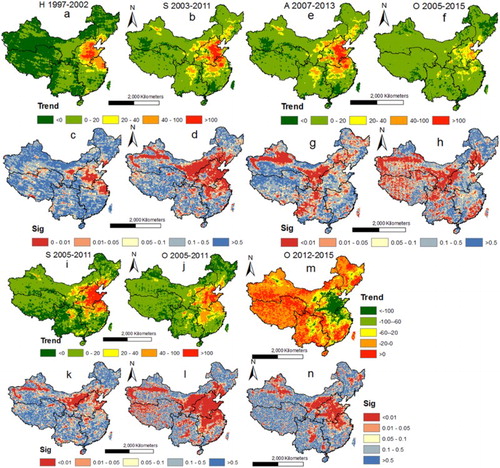
The spatial pattern of changing rate in TNCs from H, S, A and O and the significant levels are mapped in Figure 5. Generally, in NC, where TNC is the highest, large increasing trends of TNCs from H, S, O and A are mainly detected, of which the spatial extent is expanding from H (1997–2002) to S (2003–2011), but keeps contracting from S (2003–2011) to A (2007–2013) to O (2005–2015). Meanwhile, decreasing trends of TNCs from H, S, O and A are discovered in NW and TP where TNC is relatively lower. Besides, highly significant (at the significance level of 0.01) increasing trends in TNCs from H and S are detected in NC, but those from A and O in NW, TP and SW. The spatial extent of decreasing trends in NW and TP keeps contracting from H (1997–2002) to S (2003–2011) to A (2007–2013) to O (2005–2015). This is consistent with the temporal series indicated by H, S, O and A (see Figure 5(a)–(h)). Compared with TNC from S in NC (2003–2011), smaller increasing trends in TNC from O in NC (2005–2015) might be explained by the significant (at the significance level of 0.01) decreasing trends in TNC from O in NC from 2013 to 2015 (see Figure 5(m) and (n)). Though S and O indicate a similar spatial pattern of trends in TNC during 2005–2011, as the largest increasing trends are more significant in NC, however, the trends in TNC from O are more significant (at the significance level of 0.01). Also, there are slight differences between the trends in TNCs from O and S regarding the magnitude of the changing rates (see Figure 5(i)–(l)).

Figure 5. Spatial maps of changing rate and corresponding significance levels of TNC over China, unit of the trend: 10¹⁵ molecules cm⁻² yr⁻¹, Sig represents the significance level. GOME/ERS-2 (H), SCIAMACHY (S), OMI (O), GOME-2/METOP_A (A) and GOME-2/METOP_B (B).

3.4. Comparison of datasets within overlapped years

The regression results between four pairs of datasets at the country level are shown in Figure 6. Different datasets are well correlated based on the linear regressions. Overall, TNCs from A, B and S are larger than that from O, and TNC from S is larger than that from A. More specifically, TNCs from S and A have reached a good agreement, where the regression coefficient is close to 1.00. TNCs from A and B are much more similar as the regression coefficients between O&A and O&B are close. However, TNC from S is much larger than that from O as the coefficient is far away from 1.00.

Figure 6. Scatter plots and regression results between four pairs of datasets based on the multiple-year average annual TNC at the country level, the vertical axis (y) is for TNC from O, O, S, S and the horizontal axis (x) is for TNC from A, B, A, O, respectively. Unit: 10¹⁵ molecules cm⁻². GOME/ERS-2 (H), SCIAMACHY (S), OMI (O), GOME-2/METOP_A (A) and GOME-2/METOP_B (B).

Parameters of regression results between four pairs of datasets at the region level are listed in Table 2. Similar rules found at the country level between different datasets are detected at the region level as TNCs from S, A and B are larger than that from O. Moreover, comparisons at the region level further suggest that TNCs from different datasets are highly consistent in TP where the regression coefficients are close to 1.00 and the absolute gap is the minimum. The agreement of TNCs from different datasets is not desirable in NC as the regression coefficients are far from 1.00 plus the largest absolute gap. It can be concluded that TNCs from different datasets are highly consistent in TP but differ greatly in NC.

Table 2. Parameters of regression between different datasets in six regions.

Region	O&A (2007–2013)				O&B (2013–2015)				S&A (2007–2011)				S&O (2005–2011)
	a	r^2	|D|	N	a	r^2	|D|	N	a	r^2	|D|	N	a	r^2	|D|	N
NC	0.56	0.89	617	693	0.56	0.85	658	677	1.20	0.96	214	624	1.85	0.93	702	662
SE	0.65	0.93	196	691	0.77	0.89	160	689	1.22	0.97	26	686	1.59	0.97	168	684
NE	0.70	0.95	93	653	0.76	0.83	92	513	1.23	0.95	10	513	1.63	0.96	114	490
NW	0.54	0.90	24	598	0.57	0.88	36	519	1.04	0.93	4	517	1.41	0.88	6	508
SW	0.77	0.87	38	688	0.80	0.84	59	670	0.82	0.93	54	569	0.95	0.90	15	564
TP	1.00	0.82	14	675	0.77	0.7	9	641	1.02	0.87	6	378	0.95	0.80	4	667

Note: a, r², |D| and N represent coefficients, r-square of linear regression, the absolute gap (unit:10¹⁵ molecules cm⁻²) and the number of sampling points. GOME/ERS-2 (H), SCIAMACHY (S), OMI (O), GOME-2/METOP_A (A) and GOME-2/METOP_B (B).

3.5. Discussion

Five datasets have more complete records in NC where the number of missing months is less than 12. Grids with over 48-month missing records exist in part of NW by H, in SW, part of NE by S, and part of TP and NE by O. Overall, A and B products have more complete records than H, S and O. More grids with less than 12-month missing values are found in NC and SE in O, A and B products. So, changes in the selection rule may impact variation of TNC from S in NE, SW and that of TNC from O in TP, NW, but TNC in NC and SE would not be significantly influenced (Figure 7).

Figure 7. Spatial distribution of numbers of missing values on grid scale within each dataset under the predefined rule. GOME/ERS-2 (H), SCIAMACHY (S), OMI (O), GOME-2/METOP_A (A) and GOME-2/METOP_B (B).

To further confirm that the temporal trends of TNCs from five datasets are not impacted by the missing values from year to year, results based on all grids (regardless of the number of missing values) and grids with less than 12-month missing values are compared in Figure 8.

Figure 8. Comparison of temporal series of the annual TNC calculated under different grid-selection rule: (a), grids with less than 12-month missing values are selected, (b), grids are selected by the rule described in Section 2.2 and (c) all grids are included. The solid mark represents the highest level of annual TNC. Unit: 10¹⁵ molecules cm⁻². GOME/ERS-2 (H), SCIAMACHY (S), OMI (O), GOME-2/METOP_A (A) and GOME-2/METOP_B (B).

The annual TNCs by three different rules all confirm increasing trends from 1997 to 2002 by H, and increasing trends until 2011 by S, A and O, and the decreasing trends from 2011 to 2015 by O, A and B. so the trend in TNC during the past 19 years won’t be affected by the selection of grids. However, in the first circumstance (see Figure 8(a)), the TNC from S is much higher than those in the other two circumstances, as the exclusion of too many grids may cause more or less overestimation. Meanwhile, all grids included (see Figure 8(c)) result in general underestimation compared to the other two. In contrast, predefined rule utilized here has reached desirable estimation, and there are better agreements between different datasets. So we conclude that the rule applied is acceptable and reasonable. Besides, the highest level of the annual TNC in 2011 is also confirmed by three different calculations. In all, differences introduced by the selection of grids only occur in small part within the specific dataset; it won’t affect the trend of TNC as well as the year when the major changes (such as the highest level) take place.

Secondly, previous work concluded that S observed up to 40% higher NO₂ than O over fossil-fuel source regions at northern mid-latitudes, but up to 40% lower NO₂ than O over biomass burning regions in the tropics (Boersma et al. 2008). Boersma et al. (2009) also found out up to 40% higher NO₂ from S than O in summer. Meantime, Richter et al. (2011) suggested that NO₂ columns from S and A, B showed very good agreement at all latitudes and seasons, however, a small, seasonally varying difference could be explained by a systematic offset introduced by changes in the solar spectra used in the datasets. The comparison of five datasets here shows similar rules as mentioned in previous work, but there are still some seasonal and regional differences, which may be partly due to the rule selected for calculation and partly the anthropogenic sources of NO₂ over China.

Thirdly, the multiple-year average TNCs from five datasets share the similar regional difference as TNC is higher in NC and SE but lower in TP and NW, which reveals the connection between NO₂ emissions with social-economic developments. NC and SE are more developed and populated than TP and NW, automobile population, urbanization rate, intensive agricultural activities as well as energy consumption in the more-developed region may largely contribute to the NO₂ emission (Kan, Chen, and Tong 2012). Previous work suggests that TNC has been increasing over China from 1996 to 2005 (Van Der A et al. 2006) and 2006 (Zhang et al. 2007) or since 2004 (Xiao, Jiang, and Cheng 2011) based on the measurement from the satellite instruments. However, significant decreasing trends of TNC since 2011 detected in this study are undoubtedly good news for China. Since 2012 China has adopted the Ambient Air Quality Standard, and started the development of a national Air Reporting System that now includes 945 sites in 190 cities, and focus on six pollutants including NO₂ (Rohde and Muller 2015). The decrease of TNC since 2011 further confirms the far-reaching benefits of China’s effort to limit air pollution such as strengthening vehicle-emissions, promoting developments with constrained fossil-fuel use and limiting the pollutants emission of power plants and industrial activities. Besides, we believe the abrupt reduction of NO₂ in 2008 and 2009 is partly due to the Beijing 2008 Olympic Games (Yu et al. 2010) and partly the global 2008 economic depression. Yu et al. (2010) found remarkable effect of the air quality ensuring measures in reducing NO₂ pollution over Northern China during the Beijing 2008 Olympic Games.

4. Conclusions

In this study, comparisons of TNCs from five satellite datasets including GOME/ERS-2(H,1997–2002), SCIAMACHY (S, 2003–2011), OMI (O, 2005–2015), GOME-2/METOP_A (A, 2007–2013) and GOME-2/METOP_B (B, 2013–2015) were conducted in terms of the spatiotemporal changes of TNCs in Southeast (SE), Northeast (NE), Southwest (SW), Northwest (NW), North China (NC) and Tibetan Plateau (TP) over China during 1997–2015. The following conclusions have been drawn.

At the country level, H indicates an increasing trend of TNC over China since 1997, further increasing trends have been detected by S and O until the highest level of NO₂ is reached in 2011, O, A and B suggest decreasing trends of TNC after 2011 both annually and seasonally, which is mainly attributed to the government policy started in 2012. Besides, five datasets detect a seasonal pattern of winter highs and summer lows of TNCs. The connection between TNC and social-economic developments is also reflected by the regional difference of TNC as it is higher in more developed NC and SE but lower in less-developed TP and NW. Moreover, TNCs from H, S, O and A show larger increasing trends in North China.

At the region level, TNC from H has been increasing in NC and SE but decreasing in TP both annually and seasonally (1997–2002). S also suggests increasing trends of TNC in six regions both annually and seasonally except spring TNC in TP (2003–2011). While, B and O indicate decreasing trends in six regions both annually and seasonally, except annual, spring and winter TNC in TP (2013–2015). Despite the regional difference, TNC from NC contributes to the highest level of TNC from S, O and A both annually and seasonally in 2011, and TNCs from NC, SE contribute to the abrupt reductions of TNCs from S, O and A in spring and winter 2009, but in autumn 2008 at the country level. It is suggested that NC takes an important place in the variations of TNC over China. Apart from the impact of limiting NO₂ emission by government, the global economic depression and the Beijing 2008 Olympic Games are likely to cause reductions of NO₂ in 2008 and 2009.

Both temporal series and linear regressions suggest that TNCs extracted from S, A and B are larger than that from O at the country level, which may be explained by different local time of satellite sensors, the spatial resolution, as well as different retrieving methods of different datasets. Regionally, the comparison suggests TNCs from different datasets are consistent in TP but differ greatly in NC, which implies that the differences of TNCs from five satellite datasets largely result from differences in region where TNC is high.

Multi-satellite observations enable a long-term analysis of variability in tropospheric NO₂ column over China from 1997 to 2015. Comparison of datasets with different temporal coverage facilitates a better understanding of the biases among different datasets, and these biases allow for analyses combining these satellite datasets for the long-term variability of NO₂ and other air quality studies over China. In the future use of these satellite products, the potential over/underestimations and spatial variations should be taken into consideration.

Acknowledgement

The authors would like thank three anonymous reviewers for their constructive comments and suggestions for improving the quality of this paper.

Disclosure statement

No potential conflict of interest was reported by the authors.

Additional information

Funding

This research was funded by Canada National Science and Engineering Research Council (NSERC) Discovery Grant, National Natural Science Foundation of China (Nos. 41471343 and 41101315) and Ontario Trillium Foundation.

References

- Aas, W., M. Shao, L. Jin, T. Larssen, D. Zhao, R. Xiang, J. Zhang, J. Xiao, and L. Duan. 2007. “Air Concentrations and Wet Deposition of Major Inorganic Ions at Five Non-Urban Sites in China, 2001–2003.” Atmospheric Environment 41 (8): 1706–1716. doi: 10.1016/j.atmosenv.2006.10.030
- Beirle, S., U. Platt, M. Wenig, and T. Wagner. 2003. “Weekly Cycle of NO2 by GOME Measurements: A Signature of Anthropogenic Sources.” Atmospheric Chemistry and Physics 3 (6): 2225–2232. doi: 10.5194/acp-3-2225-2003
- Blond, N., K. F. Boersma, H. J. Eskes, R. J. van der A, M. Van Roozendael, I. De Smedt, G. Bergametti, and R. Vautard. 2007. “Intercomparison of SCIAMACHY Nitrogen Dioxide Observations, in Situ Measurements and Air Quality Modeling Results Over Western Europe.” Journal of Geophysical Research: Atmospheres 112, D10311. doi:10.1029/2006JD007277.
- Boersma, K. F., H. J. Eskes, and E. J. Brinksma. 2004. “Error Analysis for Tropospheric NO2 Retrieval from Space.” Journal of Geophysical Research 109, D04311. doi:10.1029/2003JD003962.
- Boersma, K. F., H. J. Eskes, R. J. Dirksen, J. P. Veefkind, P. Stammes, V. Huijnen, Q. L. Kleipool, et al. 2011. “An Improved Tropospheric NO2 Column Retrieval Algorithm for the Ozone Monitoring Instrument.” Atmospheric Measurement Techniques 4 (9): 1905–1928. doi: 10.5194/amt-4-1905-2011
- Boersma, K. F., H. J. Eskes, J. P. Veefkind, E. J. Brinksma, R. J. Van Der A, M. Sneep, G. H. J. van den Oord, et al. 2006. “Near-real Time Retrieval of Tropospheric NO2 from OMI.” Atmospheric Chemistry and Physics Discussions, European Geosciences Union 6 (6): 12301–12345. doi: 10.5194/acpd-6-12301-2006
- Boersma, K. F., D. J. Jacob, H. J. Eskes, R. W. Pinder, and J. Wang. 2008. “Intercomparison of SCIAMACHY and OMI Tropospheric NO2 Columns: Observing the Diurnal Evolution of Chemistry and Emissions from Space.” Journal of Geophysical Research: Atmospheres 113, D16S26. doi:10.1029/2007JD008816.
- Boersma, K. F., D. J. Jacob, M. Trainic, Y. Rudich, I. DeSmedt, R. Dirksen, and H. J. Eskes. 2009. “Validation of Urban NO2 Concentrations and their Diurnal and Seasonal Variations Observed from the SCIAMACHY and OMI Sensors using In Situ Surface Measurements in Israeli Cities.” Atmospheric Chemistry and Physics 9 (12): 3867–3879. doi: 10.5194/acp-9-3867-2009
- Bortoli, D., F. Ravegnani, I. K. Kostadinov, G. Giovanelli, A. Petritoli, R. Werner, A. Atanassov, and D. Valev. 2001. “Stratosphere NO2 Observation at Mid-and High Latitude Performed with Ground-Based Spectrometers.” Europe Remote Sensing 297–308. doi: 10.1117/12.413877
- Celarier, E. A., E. J. Brinksma, J. F. Gleason, J. P. Veefkind, A. Cede, J. R. Herman, D. Ionov, et al. 2008. “Validation of Ozone Monitoring Instrument Nitrogen Dioxide Columns.” Journal of Geophysical Research: Atmospheres 113 (15): 1–23.
- Chen, X. Y., and J. Mulder. 2007. “Atmospheric Deposition of Nitrogen at Five Subtropical Forested Sites in South China.” Science of the Total Environment 378 (3): 317–330. doi: 10.1016/j.scitotenv.2007.02.028
- Chen, X. Y., J. Mulder, Y. H. Wang, D. W. Zhao, and R. J. Xiang. 2004. “Atmospheric Deposition, Mineralization and Leaching of Nitrogen in Subtropical Forested Catchments, South China.” Environmental Geochemistry and Health 26 (2): 179–186. doi: 10.1023/B:EGAH.0000039580.79321.1a
- David, L. M., and P. R. Nair. 2011. “Diurnal and Seasonal Variability of Surface Ozone and NOX at a Tropical Coastal Site: Association with Mesoscale and Synoptic Meteorological Conditions.” Journal of Geophysical Research: Atmospheres 116, D10303. doi:10.1029/2010JD015076.
- Eskes, H. J., and K. F. Boersma. 2003. “Averaging Kernels for DOAS Total-Column Satellite Retrievals.” Atmospheric Chemistry and Physics, 3: 1285–1291. doi: 10.5194/acp-3-1285-2003
- Gu, B., Y. Ge, Y. Ren, B. Xu, W. Luo, H. Jiang, B. Gu, and J. Chang. 2012. “Atmospheric Reactive Nitrogen in China: Sources, Recent Trends, and Damage Costs.” Environmental Science & Technology 46: 9420–9427. doi: 10.1021/es301446g
- Han, S., H. Bian, Y. Feng, A. Liu, X. Li, F. Zeng, and X. Zhang. 2011. “Analysis of the Relationship between O3, NO and NO2 in Tianjin, China.” Aerosol Air Quality Research 11 (2): 128–139.
- Heland, J., H. Schlager, A. Richter, and J. P. Burrows. 2002. “First Comparison of Tropospheric NO2 Column Densities Retrieved from GOME Measurements and In Situ Aircraft Profile Measurements.” Geophysical Research Letters 29 (20): 441–444. doi: 10.1029/2002GL015528
- Heue, K. P., A. Richter, M. Bruns, J. P. Burrows, C. V. Friedeburg, U. Platt, I. Pundt, P. Wang, and T. Wagner. 2005. “Validation of SCIAMACHY Tropospheric NO2-Columns with AMAXDOAS Measurements.” Atmospheric Chemistry and Physics 5 (4): 1039–1051. doi: 10.5194/acp-5-1039-2005
- Irie, H., K. F. Boersma, Y. Kanaya, H. Takashima, X. Pan, and Z. F. Wang. 2012. “Quantitative Bias Estimates for Tropospheric NO2 Columns Retrieved from SCIAMACHY, OMI, and GOME-2 Using a Common Standard for East Asia.” Atmospheric Measurement Techniques 5 (10): 2403–2411. doi: 10.5194/amt-5-2403-2012
- Jiang, W. H., J. Z. Ma, P. Yang, A. Richter, J. P. Burrows, and H. Nüß. 2006. “Characterization of NO2 Pollution Changes in Beijing Using GOME Satellite Data.” Journal of Applied Meteorological Science 17 (1): 67–72. (In Chinese).
- Jo, W. K., I. H. Yoon, and C. W. Nam. 2000. “Analysis of Air Pollution in Two Major Korean Cities: Trends, Seasonal Variations, Daily 1-Hour Maximum Versus Other Hour-Based Concentrations, and Standard Exceedances.” Environmental Pollution 110 (1): 11–18. doi: 10.1016/S0269-7491(99)00284-5
- Kan, H., R. Chen, and S. Tong. 2012. “Ambient Air Pollution, Climate Change, and Population Health in China.” Environment International 42: 10–19. doi: 10.1016/j.envint.2011.03.003
- Konovalov, I. B., M. Beekmann, R. Vautard, J. P. Burrows, A. Richter, H. Nüß, and N. Elansky. 2005. “Comparison and Evaluation of Modelled and GOME Measurement Derived Tropospheric NO2 Columns Over Western and Eastern Europe.” Atmospheric Chemistry and Physics 5 (1): 169–190. doi: 10.5194/acp-5-169-2005
- Kramer, L. J., R. J. Leigh, J. J. Remedios, and P. S. Monks. 2008. “Comparison of OMI and Ground-Based In Situ and MAX-DOAS Measurements of Tropospheric Nitrogen Dioxide in an Urban Area.” Journal of Geophysical Research: Atmospheres 113, D16S39. doi:10.1029/2007JD009168.
- Krotkov, Nickolay A., Simon A. Cam, Arlin J. Krueger, Pawan K. Bhartia, and Kai Yang. 2006. “Band Residual Difference Algorithm for Retrieval of SO2 from the Aura Ozone Monitoring Instrument (OMI)." IEEE Transactions on Geoscience and Remote Sensing 44 (5): 1259–1266. doi: 10.1109/TGRS.2005.861932
- Kurokawa, J., T. Ohara, T. Morikawa, S. Hanayama, G. Janssens-Maenhout, T. Fukui, K. Kawashima, and H. Akimoto. 2013. “Emissions of Air Pollutants and Greenhouse Gases Over Asian Regions During 2000-2008: Regional Emission Inventory in Asia (REAS) Version 2.” Atmospheric Chemistry and Physics 13 (21): 11019–11058. doi: 10.5194/acp-13-11019-2013
- Lamsal, L. N., R. V. Martin, A. Van Donkelaar, M. Steinbacher, E. A. Celarier, E. Bucsela, E. J. Dunlea, and J. P. Pinto. 2008. “Ground-Level Nitrogen Dioxide Concentrations Inferred from the Satellite-Borne Ozone Monitoring Instrument.” Journal of Geophysical Research Atmospheres 113 (16): 1–15.
- Lauer, A., M. Dameris, A. Richter, and J. P. Burrows. 2002. “Tropospheric NO2 Column: A Comparison between Model and Retrieved Data from GOME Measurements.” Atmospheric Chemistry and Physics 2 (1): 67–78. doi: 10.5194/acp-2-67-2002
- Liu, X., Y. Zhang, W. Han, A. Tang, J. Shen, Z. Cui, P. Vitousek, et al. 2013. “Enhanced Nitrogen Deposition over China.” Nature 494 (7438): 459–462. doi: 10.1038/nature11917
- Martin, R. V., C. E. Sioris, K. Chance, T. B. Ryerson, T. H. Bertram, P. J. Wooldridge, R. C. Cohen, J. A. Neuman, A. Swanson, and F. M. Flocke. 2006. “Evaluation of Space-Based Constraints on Global Nitrogen Oxide Emissions with Regional Aircraft Measurements Over and Downwind of Eastern North America.” Journal of Geophysical Research: Atmospheres 111, D15308. doi:10.1029/2005JD006680.
- Meng, X., L. Chen, J. Cai, B. Zou, C. F. Wu, Q. Fu, Y. Zhang, Y. Liu, and H. D. Kan. 2015. “A Land Use Regression Model for Estimating the NO2 Concentration in Shanghai, China.” Environmental Research 137: 308–315. doi: 10.1016/j.envres.2015.01.003
- Richter, A., M. Begoin, A. Hilboll, and J. P. Burrows. 2011. “An Improved NO2 Retrieval for the GOME-2 Satellite Instrument.” Atmospheric Measurement Techniques 4 (6): 1147–1159. doi: 10.5194/amt-4-1147-2011
- Richter, A., J. P. Burrows, H. Nüß, C. Granier, and U. Niemeier. 2005. “Increase in Tropospheric Nitrogen Dioxide Over China Observed from Space.” Nature 437 (7055): 129–132. doi: 10.1038/nature04092
- Rohde, R. A., and R. A. Muller. 2015. “Air Pollution in China: Mapping of Concentrations and Sources.” Plos One 10 (8): e0135749. doi:10.1371/journal.pone.0135749.
- Schaub, D., K. F. Boersma, J. W. Kaiser, A. K. Weiss, D. Folini, H. J. Eskes, and B. Buchmann. 2006. “Comparison of GOME Tropospheric NO2 Columns with NO2 Profiles Deduced from Ground-Based In Situ Measurements.” Atmospheric Chemistry and Physics 6 (11): 3211–3229. doi: 10.5194/acp-6-3211-2006
- Schaub, D., D. Brunner, K. F. Boersma, J. Keller, D. Folini, B. Buchmann, H. Berresheim, and J. Staehelin. 2007. “SCIAMACHY Tropospheric NO2 Over Switzerland: Estimates of NOx Lifetimes and Impact of the Complex Alpine Topography on the Retrieval.” Atmospheric Chemistry and Physics 7 (23): 5971–5987. doi: 10.5194/acp-7-5971-2007
- Uno, I., Y. He, T. Ohara, K. Yamaji, J. I. Kurokawa, M. Katayama, Z. Wang, et al. 2007. “Systematic Analysis of Interannual and Seasonal Variations of Model-Simulated Tropospheric NO2 in Asia and Comparison with GOME-Satellite Data.” Atmospheric Chemistry and Physics 7 (6): 1671–1681. doi: 10.5194/acp-7-1671-2007
- Valks, P., G. Pinardi, A. Richter, J. C. Lambert, N. Hao, D. Loyola, M. Van Roozendael, and S. Emmadi. 2011. ““Operational Total and Tropospheric NO2 Column Retrieval for GOME-2.” Atmospheric Measurements Techniques Discussion 4: 1617–1676. doi: 10.5194/amtd-4-1617-2011
- Van Der A, R. J., D. H. M. U. Peters, H. Eskes, K. F. Boersma, M. Van Roozendael, I. De Smedt, and H. M. Kelder. 2006. “Detection of the Trend and Seasonal Variation in Tropospheric NO2 Over China.” Journal of Geophysical Research: Atmospheres 111, D12317. doi:10.1029/2005JD006594.
- Velders, G. J., C. Granier, R. W. Portmann, K. Pfeilsticker, M. Wenig, T. Wagner, U. Platt, A. Richter, and J. P. Burrows. 2001. “Global Tropospheric NO2 Column Distributions: Comparing Three-Dimensional Model Calculations with GOME Measurements.” Journal of Geophysical Research: Atmospheres 106: 12643–12660. doi: 10.1029/2000JD900762
- Wang, S., B. Zhou, Z. Wang, S. Yang, N. Hao, T. Trautmann, and L. M. Chen. 2012. “Remote Sensing of NO2 Emission from the Central Urban Area of Shanghai (China) Using the Mobile DOAS Technique.” Journal of Geophysical Research Atmospheres 117 (D13): 110–117. doi: 10.1029/2011JD016983
- Xiao, Z. Y., H. Jiang, and M. M. Cheng. 2011. “Characteristics of Atmospheric NO2 Over China Using OMI Remote Sensing Data.” Acta Scientiae Circumstantiate 31 (10): 2080–2090. (In Chinese).
- Xu, W., X. S. Luo, Y. P. Pan, L. Zhang, A. H. Tang, J. L. Shen, Y. Zhang, et al. 2015. “Quantifying Atmospheric Nitrogen Deposition through a Nationwide Monitoring Network across China.” Atmospheric Chemistry and Physics 15 (21): 12345–12360. doi: 10.5194/acp-15-12345-2015
- Yu, H., P. Wang, X. Zong, X. Li, and D. Lü. 2010. “Change of NO2 Column Density Over Beijing from Satellite Measurement during the Beijing 2008 Olympic Games.” Chinese Science Bulletin 55 (3): 308–313.
- Zhang, Q., G. N. Gen, S. W. Wang, A. Richter, and K. B. He. 2012. “Satellite Remote Sensing of Changes in NOx Emissions over China: 1996-2010.” Chinese Science Bulletin 57 (16): 1446–1453. (In Chinese).
- Zhang, X., P. Zhang, Y. Zhang, X. Li, and H. Qiu. 2007. “The Trend, Seasonal Cycle, and Sources of Tropospheric NO2 Over China during 1997–2006 Based on Satellite Measurement.” Science in China Series D: Earth Sciences 50 (12): 1877–1884. doi: 10.1007/s11430-007-0141-6