
ABSTRACT
Mapping geographic concentrations of quaternary industries (QIs) may help to assess regional performance and formulate informed development policies. However, fine resolution data on QIs concentrations are sparsely reported. Thus, for the year 2010, only 45% of all NUTS3 regions (i.e. regions of the third and most detailed level of the Nomenclature of Units for Territorial Statistics of the EU) provide relevant information. In this study, we investigate a possibility that artificial light-at-night (ALAN), captured by satellite sensors, can help to identify geographic concentrations of QIs. In this study, we use year-2010 NUTS3 Eurostat data, and combine them with data on ALAN intensities, obtained from the U.S. Defense Meteorological Satellite Program (US-DMSP) for the years 2000 and 2010. In both ordinary least squares (OLS) and spatial dependency (SD) models, ALAN emerged as a statistically significant predictor (t = 8.392–14.608; P < .01), helping to explain, along with other predictors, up to 75% of QIs regional variation. The obtained models and regional data presently available enabled estimates of QIs concentrations for European NUTS3 regions with missing data.
1. Introduction
Quaternary industries (QIs), formed by high technology firms, research, educational and professional activities, are widely considered the main driving force behind modern economic growth (Varga and Schalk Citation2004; Acs and Plummer Citation2005; Mueller Citation2006; Yusuf and Nabeshima Citation2007; Acs, de Groot, and Nijkamp Citation2013). The identification of regional concentrations of QIs thus becomes an important thrust of regional studies and policy design.
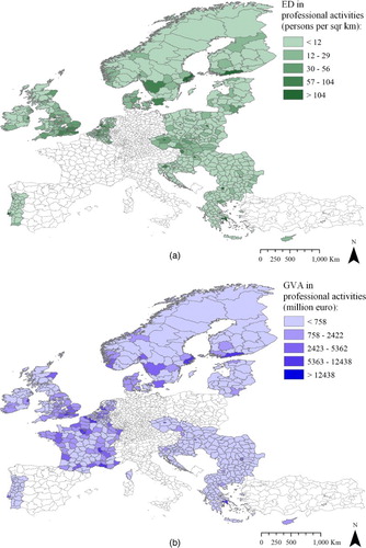
However, relatively little information is currently available on the geographic concentrations of QIs. Thus, for the year 2010, only about 45% of European NUTS3 regions provide information on employment density and gross value added (GVA) by QIs (see ); for the year 2000, corresponding data are available for about 20% of all NUTS3 regions only.
Figure 1. Distribution of professional activities across European NUTS3 regions with data available for year 2010: (a) Employment density (ED), persons per km2; (b) GVA, million €. Source: Eurostat Portal (EP Citation2014).
In the absence of reported data, several indirect approaches are used to assess QIs geographic patterns. Some of these estimation approaches are based on the number of patents, innovation and publication counts and on various human capital indices (Fagerberg Citation1987; Acs, Anselin, and Varga Citation2002; Crescenzi, Rodríguez-Pose, and Storper Citation2012; Capello and Lenzi Citation2013). However, the main difficulty associated with this approach is data availability. The matter is that data on human capital and local innovation activities are mainly available for relatively coarse geographic units, such as countries and regions (Acs, Anselin, and Varga Citation2002). In addition, there are difficulties to implement inter-regional comparison, especially for different time periods, due to differences in patent policies and innovation/publication counts (Jaffe Citation2000; Burk and Lemley Citation2003; Archibugi and Coco Citation2004; Schofer and Meyer Citation2005; Murphy and Siedschlag, Citation2011).
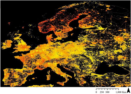
In this study, we investigate a possibility that artificial light-at-night (ALAN), emitted by various economic activities and captured by satellite sensors (see ), can help to identify, with a reasonable degree of accuracy, geographic concentrations of QIs.
Figure 2. ALAN levels detected by US DMSP satellites in 2010. Source: Mapped using US DMSP (NOAA Citation2014) data.
In the past years, ALAN satellite measurements were used in health studies (Kloog et al. Citation2007, Citation2009, Citation2010), in demographic analysis (Elvidge et al. Citation1997; Imhoff et al. Citation1997; Sutton et al. Citation2001; Anderson et al. Citation2010), and in studies of economic performance of countries and regions (Doll, Muller, and Elvidge Citation2000; Sutton, Elvidge, and Ghosh Citation2007; Henderson, Storeygard, and Weil Citation2009; Ghosh et al. Citation2010; Kulkarni et al. Citation2011; Mellander et al. Citation2013). Several empirical studies also investigated the association between ALAN and on-ground economic concentrations, either generalized (Ebener et al. Citation2005; Doll, Muller, and Morley Citation2006; Bhandari and Roychowdhury Citation2011) or industry-specific (Rybnikova and Portnov Citation2014, Citation2015).
However, to the best of our knowledge, no studies, carried out to date, have attempted to investigate whether ALAN information can be used for the identification of QIs industries, measured in terms of employment density or GVA. The present analysis attempts to fill this gap.
As we hypothesize, due to high concentration of workforce, intensive lighting required and geographic clustering of service-oriented and entertainment facilities around QIs, such industries emit nighttime light of high intensities, being significantly higher than the nighttime light emitted by traditional industries and residential areas. As a result, QIs concentrations can expectedly be identified, with a reasonable degree of accuracy, by ALAN intensities they emit (upon controlling for GDPpc and several locational attributes of geographic areas).
The rest of the paper is organized as follows. We start by describing our statistical methods, research variables and data sources. Next, we report our results on the strength of association between QIs and ALAN, comparing it with the strength of association between ALAN and primary, secondary and tertiary economic concentrations. We conclude our analysis by restoring the missing data on QIs concentrations in Europe, using available ALAN information and basic socio-demographic and geographic attributes of European NUTS3 regions.
2. ALAN-economic activity associations
In an early study, Ebener et al. (Citation2005) analyzed, apparently for the first time, the strength of association between economic development of countries and ALAN. The authors of the study examined 171 countries across the globe, and found that satellite-detected ALAN intensities helped to explain up to 80% of GDPpc variance associated with agriculture. In another study, Doll with co-authors (Citation2006) examined NUTS2 regions in 11 European countries and revealed that the association between nighttime light radiance and GDP generated by general economic sectors was statistically significant. In the Netherlands, for instance, R2 measuring these associations were found to be equal 0.83 for primary industries (PI), 0.84 for agriculture and 0.89 for services.
Bhandari and Roychowdhury (Citation2011) used year 2008 satellite-detected ALAN intensities in conjunction with socio-economic data obtained for 593 districts in India. As the authors of this study found, ALAN intensities, jointly with population size and a range of dummies, helped to explain up to 73% of GDP variance in primary and secondary sectors and up to 87% of GDP variance in the tertiary sector.
In two separate studies, Rybnikova and Portnov (Citation2014, Citation2015) analyzed European NUTS3 regions and came to the conclusion that satellite-measured ALAN intensities may help to identify remotely regional concentrations of several economic activities, helping to explain (together with socio-economic and geographic attributes of NUTS3 regions) up to 94% of geographic variation of different economic activities. However, to the best of our knowledge, ALAN association with QIs has never been investigated to date and mutually compared with the strength of association between ALAN and primary, secondary and tertiary industries (TI), which is the main thrust of this study.
3. Research methods
3.1. Study area
In the early 1970s, the Eurostat established the Nomenclature of Units for Territorial Statistics (also known as NUTS), aimed at collecting and analyzing regional statistics (EP Citation2014). The entire territory of Europe is subdivided into three different NUTS levels – NUTS1, NUTS2 and NUTS3, – with NUTS regions of the higher hierarchy (i.e. NUTS1 and NUTS2) being subdivided into smaller, NUTS3 regional subdivisions. All member states of the EU, candidate countries and European Free Trade Association (EFTA) countries (including Iceland, Norway, Principality of Liechtenstein and Switzerland), subdivided into NUTS3 regions (see ). In the present study, we use the NUTS3 Eurostat Portal (EP) data for the year 2010, which provide the most comprehensive regional coverage.
3.2. Research variables
Employment density (ED, measured in persons per km2) and GVA (in million €) by quaternary, tertiary, secondary and primary sectors in NUTS3 regions are used in the present study as dependent variables. In particular, we chose four types of economic activities, grouped according to the Statistical Classification of Economic Activities in the EU (EMS Citation2014) as typical representatives of different industrial groups: mining and quarrying (PI); manufacturing (secondary industries, SI); wholesale and retail trade, repair of motor vehicles and motorcycles, accommodation and food services (TI), and professional, scientific and technical activities, administrative and support service activities (QI). Since we found considerable deviations from normality in the original data, we applied Box-Cox transformations to the original values of ED and GVA (see Appendix 1).
In addition to ALAN intensities (see Subsection on ALAN data), the following variables were used in the analysis as potential predictors for the observed industrial concentrations in the NUTS3 regions: per capita GDP (€), population density (persons per km2), elevation above sea level (estimated for NUTS3 centroids in meters), distances to the seashore, rail, nearest major populations center (with more than 500,000 residents) and to the nearest river (km) and average seasonal temperatures (°C).Footnote1 These data were either obtained from the EP (Citation2013) or calculated in the ArcGIS software.
In empirical studies, per capita GDP and population density are often used as general indicators of the quality of life, local productivity, urbanization and so on. (see inter alia Han and Naeher Citation2006; Rappaport Citation2006; Ortiz and Cummins Citation2011). In the present study, we use these variables as proxies for a place’s ability to attract economic activities, considering that high population densities can stimulate industrial development via ensuring sufficient labor force concentration and diversity (Portnov and Schwartz Citation2009). By the same token, high GDPpc, reflecting advanced development levels (Daniele and Marani Citation2011), can also attract highly qualified workforce and thus stimulate further industrial development, specifically in the QI sector.
As well established, locational attributes of geographic areas contribute to the locational patterns of different economic activities. For instance, elevation is strongly associated with mining and quarrying (Wright and Stow Citation1999). Primary sector is also known to be influenced by seasonal temperatures (Reidsma et al. Citation2010). Heavy manufacturing is often concentrated near the seashore, and major rivers, which helps to minimize transportation costs, while good roads are needed to facilitate trade (Duranton, Morrow, and Turner Citation2013). Concurrently, professional and scientific activities are often concentrated in major cities, which are loci of population and productivity (Cuadrado-Roura and Rubalcaba-Bermejo Citation1998; Henderson Citation2010).
The above-mentioned variables were included into the models via a two-step process: In the first step, all the above-mentioned potential predictors were introduced into the models simultaneously, while at the second stage of the analysis, only statistically significant predictors (P < .05) with acceptable multicollinearity levels (VIF < 3) were retained in the models (see the subsection on Statistical analysis).
3.3. ALAN data
ALAN intensity data, which we used in our study as a potential marker for industrial concentrations, were obtained from the U.S. Defence Meteorological Satellite Program (NOAA Citation2014).Footnote2 The DMSP satellites provide continuous reading of the entire Earth surface during nighttime, as they orbit around the globe. The satellite images, used in our study, were constructed by the DMSP by averaging daily readings of the satellite sensors and removing the cloud cover. The DMSP satellite’s overpass is at 19:30, at the polar orbit of 850 km altitude; it has a 3000 km swath and low light imaging detection limit of ≈ 5 × 10⁻¹⁰ W cm−2 sr−1 (Elvidge et al. Citation2013; NOAA Citation2014). In particular, we used radiance calibrated nighttime light emission data,Footnote3 produced by satellites F16 and F12–F15 for the years 2010 and 2000, respectively. The images contain 43,201 × 16,801 pixels, and are of 30 arc-second per pixel resolution. Upon calculating average ALAN levels for the NUTS3 regions, performed using pixel-by-pixel averaging, the average ALAN values were estimated for all NUTS3 regions, and found to be in the range between 1.67 and 448.22 dimensionless units (Mean = 32.55, SD = 53.10) for the year 2010, and in the range between 0.18 and 1396.25 dimensionless units (Mean = 36.53, SD = 78.36) for the year 2000.
3.4. Statistical analysis
In the initial stage of our analysis, we used ordinary least squares (OLS) regressions, to explore associations between the quaternary, tertiary, secondary and primary industries and ALAN levels, controlling for other predictors potentially affecting industrial concentrations. The generic model we used during the first stage of the analysis was as follows:(1) where
= measure of concentration, estimated as either employment density (ED) and gross value-added (GVA) metrics for quaternary, tertiary, secondary and primary sectors hosted by NUTS3 regions; b0, b1 and vector b are regression coefficients; ALAN = average ALAN intensities emitted from NUTS3 regions (see the subsection on ALAN data); PP = vector of potential predictors (see Subsection on Research variables), and ε = random error term.
To address the issue of endogeneity potentially reflecting the fact that ALAN results from industrial concentrations, the 2-Stage Least Squares (2-SLS) regressions were used. According to this technique, so-called ‘instrumental’ predictors are used to estimate the values of potentially endogenous variables (such as ALAN vs. industrial concentrations), and these computed values are then used in the model reruns (IBM SPSS Citation2014).
We also used spatial dependency models. The use of these models was necessitated by the fact that the analysis of the regression residuals from the OLS and 2-SLS models, performed using the Moran’s I test (Ullah and Giles Citation1998), indicated a high degree of spatial auto-correlation (with Z-Moran’s I ranging from 8.460 to 16.057; P < .01 – see ), which can potentially affect the robustness of regression estimates (Fotheringham and Rogerson Citation2009). Eventually, we chose the spatial error (SE) models, as providing better fit and generality:(2) where λ = spatial error coefficient; ξ = the vector of error terms, spatially weighted using the weights matrix (W) and ζ = vector of uncorrelated error terms.
Table 1. Factors affecting economic performance of NUTS3 regions (Method – OLS regression; dependent variable – GVA, million euro, Box-Cox transformeda).
To calculate W, we used the ‘queen’ neighborhood matrix that defines neighboring regions as those with either a shared border or a common vertex (GeoDa Citation2014), as commonly done in empirical studies of geographically distributed data (see inter alia Pacheco and Tyrrel Citation2002; Roux et al. Citation2007). To estimate the ALAN contribution to the observed variation of economic activities, we applied the F-test of R2-change.
4. Results
4.1. General trends
reports the associations between ALAN intensities and different industrial concentrations. In the diagrams, ALAN intensities are shown on a logarithmic scale, which use helps to illustrate the observed associations more clearly. As shows, in terms of both ED and GVA, QI-ALAN association appears to be stronger than those detected for PI, SI and TI regional concentrations (R2 = 0.436–0.465 vs. R2 = 0.054–0.398). Apparently, the strength of this association is affected by high concentrations of labor force and more intensive lighting required by QIs and collocated services and entertainment activities.
Figure 3. Associations between ALAN and primary (a), secondary (b), tertiary (c) and quaternary (d) industrial concentrations in European NUTS3 regions. Source: Eurostat Portal (EP Citation2014) and US DMSP (NOAA Citation2014).
4.2. Multivariate analysis – OLS and 2SLS models
reports multivariate OLS regressions for PI-ALAN, SI-ALAN, TI-ALAN and QI-ALAN associations, controlled for several potential predictors, such as GDPpc, population density, elevation above sea level, distances to the closest main city, seashore, major rivers, rail and average seasonal temperatures. Since the models estimated for employment density and GVA are essentially similar, only models with GVA as the dependent variable are reported in . Part A in reports the models, to which all potential predictors are included, while Part B in reports the models incorporating only statistically significant variables (P < .05) with accepted levels of multicollinearity (VIF < 3).
As shows, ALAN appears to be a statistically significant and positive predictor for GVA in all economic sectors under analysis (t = 8.497–14.608; P < .01). However, the strength of this association appears to be higher for QI-ALAN than for PI-ALAN, SI-ALAN and TI-ALAN associations (t = 10.155 vs. t = 8.497–9.424; see , Part A; and t = 14.608 vs. t = 9.856–11.557; see , Part B). The overall model fit is also better in the QI-ALAN model, compared to that in the PI, SI and TI models (R2 = 0.679–0.710 vs. R2 = 0.213–0.621; see ). The significant contribution of ALAN to the QI model is confirmed by the F-test of R2-change (ΔR2 = 0.108, F = 213.390; P < .01; see Model 8; ).
Table 2. F-test for R2-change across different prediction models.
The 2-SLS models, reported in , are essentially similar to the OLS models, reported in , Part B, indicating that our estimates are robust.
Table 3. Factors affecting economic performance of NUTS3 regions (Method – 2-SLS) regression; dependent variables: Step 1 – Ln(ALAN), Step 2 – economic activities’ GVA, million euro).
4.3. Spatial dependency models
reports spatial error models, estimated in the GeoDaTMv1.6.6.1 software, using the ‘queen’ neighborhood matrix (GeoDa Citation2014). These models are also essentially similar to the OLS models reported in , Part B, and show that ALAN is a stronger predictor for QIs (z = 12.049; P < .01) than for TI, SI and PI industrial concentrations (z = 8.983–9.691; P < .01). In particular, in these models, ALAN, together with other explanatory variables, helps to explain up to 74% of QIs’ regional variation (R2 = 0.739), compared to 48.5–67.4% of regional variation, explained for other types of industrial concentrations.
Table 4. Factors affecting economic performance of NUTS3 regions (Method – SE regression; dependent variable – GVA rates; only statistically significant predictors with low VIF values are included).
4.4. Restoring data on QI geographical concentrations
We restored missing data on QIs regional concentrations (see ) in several stages. First, we selected a random sample of 10% of NUTS3 regions with available data, and re-estimated Model 8 (see , Part B) for the rest of 90% of NUTS3 regions with available data (see (b)). Next, we applied the re-estimated model to the preselected 10% of the cases. Next, we used a t-test to estimate whether the difference between the actual values and the model estimates is statistically different from zero. As the t-test showed, the assessed difference did not differ from zero significantly (t = −0.898; P = .372), thus indicating that our model is essentially robust. We also calculated the root mean square error (RMSE) for the actual and estimated values of the preselected 10% of cases. The calculated RMSE value equaled 1.131, which is lower than the corresponding value of 1.148, obtained for the whole set of observations (see Model 8, , Part B), and lower than the value of 1.209, obtained for the training set of 90% cases.
The same procedure of validation was applied to the year-2000 model (see Appendix 2), indicating that the difference between actual and estimated values for the control subset of 10% of NUTS3 regions did not differ significantly from zero (t = −0.250; P = .804); the RMSE value was found to be equal 0.810 vs. 0.857 for the whole set of cases (see Appendix 2) and 0.866 for the training set.
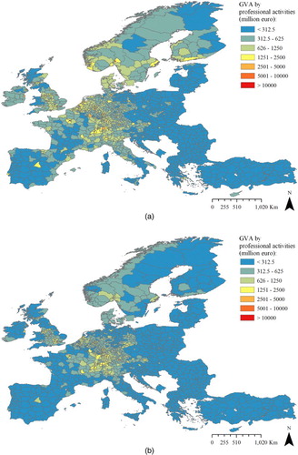
At the next step, we used the available data on ALAN, and other readily available attributes of NUTS3 regions for the years 2010 and 2000Footnote4 (i.e. GDPpc, distance to the seashore, average July temperature – see Appendix 1), to estimate QIs GVA levels for European regions with missing data.Footnote5 The estimation results are reported in , separately for the year 2010 ((a)) and for the year 2000 ((b)).
Figure 4. Estimated QIs concentrations (GVA, million euro) for European NUTS3 regions: (a) year 2010 estimates; (b) year 2000 estimates.
5. Discussion and conclusions
In the present study, we investigated a possibility that data on ALAN intensities, collected by satellite sensors, can be used to restore missing information on QIs regional concentrations. As the present analysis shows, ALAN intensities, together with other explanatory variables, such as GDPpc and geographic attributes of NUTS3 regions, helped to explain up to 74% of QIs’ regional variation. We used our models to restore missing information on on-ground concentrations of QIs GVA in NUTS3 European regions.
The analysis points out at a strong association between QIs (measured by both employment density and GVA) and ALAN, which generally coincides with the results of other studies which investigated the association of ALAN with regional economic performance (see, inter alia, Doll, Muller, and Morley Citation2006; Bhandari and Roychowdhury Citation2011; Rybnikova and Portnov Citation2014, Citation2015).
Our results may be used to reconstruct missing information on on-ground QIs concentrations, by combining ALAN intensities with easily calculated or readily available data, such as basic demographic and geographic attributes of geographic areas. Reconstructing this information may help to identify gaps in regional development, to perform policy evaluation requiring QIs data, and to formulate prospective regional development policies.
Several limitations of the present study ought to be mentioned. First, the study was performed for the European NUTS3 regions, characterized by relatively high levels of development. The strengths of the ALAN-QIs association should therefore be re-investigated elsewhere before applying the observed associations to other regions. Second, study results, obtained using US-DMSP input data, should be reanalyzed using VIIRS sensor data, which have recently become available from the Suomi National Polar Partnership (SNPP) satellite (Elvidge et al. Citation2013). In particular, future studies should attempt to determine whether the models we obtained for different types of economic activities can be further improved by using nighttime satellite images of higher spatial resolution and of lower light detection limit.
Disclosure statement
No potential conflict of interest was reported by the authors.
ORCID
Natalya A. Rybnikova http://orcid.org/0000-0002-3135-6865
Boris A. Portnov http://orcid.org/0000-0003-1537-0832
Additional information
Funding
Notes
1 In the initial stages of the analysis, we used average temperatures in July and January as predictors for industrial concentrations. Due to a multicollinearity consideration, these variables were analyzed separately. In the final models, only the best-performing seasonal variables are reported, that is, January temperatures for PIs and SIs and July temperatures for QIs. In the model for TIs, none of the temperatures emerged as statistically significant predictors.
2 ALAN emitted by on-ground economic activities cannot be viewed as an independent factor per se, due to the fact that ALAN results from industrial concentrations, potentially leading to endogeneity (Antonakis et al. Citation2014). To address the issue, we used in the analysis both OLS and 2-Stage Least Squares (2-SLS) regressions (see the subsection on Statistical analysis).
3 As previously mentioned, we used in this analysis only calibrated ALAN images available for the years 2000 and 2010. Although un-calibrated ALAN images are also available (NOAA Citation2016), these images have a problem of light saturation (Hsu et al. Citation2015), which restricts their use for the identification of QIs, which are expected to emit nighttime light of high intensity.
4 Estimates for the year 2000 are based on Model 8A, reported in Appendix B. This model is essentially similar to Model 8 (, part B); it uses the same predictors, but is based on the year 2000 data.
5 For some NUTS3 regions, GDPpc data, needed as model inputs, were unavailable. In particular, in the year 2010, such data were missing for NUTS3 regions in Turkey, Italy and Switzerland, while for 2000, no NUTS3-specific GDPpc were available for Turkey, Poland, Croatia, Spain, Italy, Germany, Norway, United Kingdom, Netherlands and Switzerland. For these countries, we used GDPpc values, available for larger areas, such as NUTS2, and NUTS1, depending on data availability.
References
- Acs, Z. J., L. Anselin, and A. Varga. 2002. “Patents and Innovation Counts as Measures of Regional Production of New Knowledge.” Research policy 31 (7): 1069–1085. doi: 10.1016/S0048-7333(01)00184-6
- Acs, Z. J., H. L. de Groot, and P. Nijkamp, eds. 2013. The Emergence of the Knowledge Economy: A Regional Perspective. Springer Science & Business Media.
- Acs, Z. J., and L. A. Plummer. 2005. “Penetrating the “Knowledge Filter” in Regional Economies.” The Annals of Regional Science 39 (3): 439–456. doi: 10.1007/s00168-005-0245-x
- Anderson, S. J., B. T. Tuttle, R. L. Powell, and P. C. Sutton. 2010. “Characterizing Relationships Between Population Density and Nighttime Imagery for Denver, Colorado: Issues of Scale and Representation.” International Journal of Remote Sensing. 21: 5733–5746. doi: 10.1080/01431161.2010.496798
- Antonakis, J., S. Bendahan, P. Jacquart, and R. Lalive. 2014. “Causality and Endogeneity: Problems and Solutions.” Accessed March 2014. http://www.oxfordhandbooks.com/view/10.1093/oxfordhb/9780199755615.001.0001/oxfordhb-9780199755615-e-007
- Archibugi, D., and A. Coco. 2004. “A New Indicator of Technological Capabilities for Developed and Developing Countries (ArCo).” World Development 32 (4): 629–654. doi: 10.1016/j.worlddev.2003.10.008
- Bhandari, L., and K. Roychowdhury. 2011. “Night Lights and Economic Activity in India: A Study Using DMSP-OLS Night Time Images.” Proceedings of the Asia-Pacific Advanced Network 32: 218–236. doi: 10.7125/APAN.32.24
- Burk, D. L., and M. A. Lemley. 2003. “Policy Levers in Patent Law.” Virginia Law Review 89: 1575–1696. doi: 10.2307/3202360
- Capello, R., and C. Lenzi. 2013. Territorial Patterns of Innovation: An Inquiry on the Knowledge Economy in European Regions. New York: Routledge.
- Crescenzi, R., A. Rodríguez-Pose, and M. Storper. 2012. “The Territorial Dynamics of Innovation in China and India.” Journal of Economic Geography 12 (5): 1055–1085. doi: 10.1093/jeg/lbs020
- Cuadrado-Roura, J. R., and L. Rubalcaba-Bermejo. 1998. “Specialization and Competition Amongst European Cities: A New Approach Through Fair and Exhibition Activities.” Regional studies 32 (2): 133–147. doi: 10.1080/00343409850123026
- Daniele, V., and U. Marani. 2011. “Organized Crime, the Quality of Local Institutions and FDI in Italy: A Panel Data Analysis.” European Journal of Political Economy 27 (1): 132–142. doi: 10.1016/j.ejpoleco.2010.04.003
- Doll, C. N. H., J. P. Muller, and C. D. Elvidge. 2000. “Nighttime Imagery as a Tool for Global Mapping of Socioeconomic Parameters and Greenhouse Gas Emissions.” A Journal of the Human Environment 29 (3): 157–162. doi: 10.1579/0044-7447-29.3.157
- Doll, C. N. H., J. P. Muller, and J. G. Morley. 2006. “Mapping Regional Economic Activity from Night-Time Light Satellite Imagery.” Ecological Economics 57 (1): 75–92. doi: 10.1016/j.ecolecon.2005.03.007
- Duranton, G., P. Morrow, and M. Turner. 2013. “Roads and Trade: Evidence from the US.” CEPR Discussion Paper No. DP9393. Accessed April 2014. http://ssrn.com/abstract=2235491
- Ebener, S., C. Murray, A. Tandon, and C. D. Elvidge. 2005. “From Wealth to Health: Modeling the Distribution of Income Per Capita at the Subnational Level using Nighttime Light Imagery.” International Journal of Health Geographics. Accessed February 2014. http://www.ij-healthgeographics.com/content/4/1/5
- Elvidge, C., K. Baugh, E. Kihn, H. Kroehl, E. Davis, and C. Davis. 1997. “Relation Between Satellite Observed Visible-Near Infrared Emissions, Population, Economic Activity and Electric Power Consumption.” International Journal of Remote Sensing 18: 1373–1379. doi: 10.1080/014311697218485
- Elvidge, C., K. Baugh, M. Zhizhin, and F. Hsu. 2013. “Why VIIRS Data Are Superior to DMSP for Mapping Night-Time Lights.” Proceedings of the Asia-Pacific Advanced Network 35: 62–69. doi: 10.7125/APAN.35.7
- Eurostat Portal (EP). 2013. Statistical Databases. Accessed December 2013. http://epp.eurostat.ec.europa.eu/portal/page/portal/statistics/search_database.
- Eurostat Portal (EP). 2014. History of NUTS. Accessed January 2014. http://epp.eurostat.ec.europa.eu/portal/page/portal/nuts_nomenclature/documents
- Eurostat’s Metadata Server (EMS). 2014. “Statistical Classification of Economic Activities in the European Community.” Rev 2 (2008). Accessed January 2014. http://ec.europa.eu/eurostat/ramon/nomenclatures/index.cfm?TargetUrl=LST_NOM_DTL_LINEAR&IntCurrentPage=1&StrNom=NACE_REV2&StrLanguageCode=EN
- Fagerberg, J. 1987. “A Technology Gap Approach to Why Growth Rates Differ.” Research policy 16 (2): 87–99. doi: 10.1016/0048-7333(87)90025-4
- Fotheringham, A. S., and P. A. Rogerson. 2009. The SAGE Handbook of Spatial Analysis. 528.
- GeoDa Center for Geospatial Analysis and Computation (GeoDa). 2014. Glossary of Key Terms. Accessed March 2014. https://geodacenter.asu.edu/node/390
- Ghosh, T., R. Powell, C. D. Elvidge, K. E. Baugh, P. C. Sutton, and S. Anderson. 2010. “Shedding Light on the Global Distribution of Economic Activity.” The Open Geography Journal 3: 147–160. doi: 10.2174/1874923201003010147
- Han, X., and L. P. Naeher. 2006. “A Review of Traffic-Related Air Pollution Exposure Assessment Studies in the Developing World.” Environment international 32 (1): 106–120. doi: 10.1016/j.envint.2005.05.020
- Henderson, J. V. 2010. “Cities and Development.” Journal of Regional Science 50 (1): 515–540. doi: 10.1111/j.1467-9787.2009.00636.x
- Henderson, J. V., A. Storeygard, and D. N. Weil. 2009. Measuring Economic Growth from Outer Space. Accessed March 2014. http://www.nber.org/papers/w15199
- Hsu, F. C., K. E. Baugh, T. Ghosh, M. Zhizhin, and C. D. Elvidge. 2015. “DMSP-OLS Radiance Calibrated Nighttime Lights Time Series with Intercalibration.” Remote Sensing 7 (2): 1855–1876. doi: 10.3390/rs70201855
- IBM SPSS Statistics (IBM SPSS). 2014. Two-Stage Least-Squares Regression. Accessed March 2014. http://gsb137389-3193:49488/help/index.jsp?topic=/com.ibm.spss.statistics.help/idh_tsls.htm
- Imhoff, M. L., W. T. Lawrence, D. C. Stutzer, and C. D. Elvidge. 1997. “A Technique for Using Composite DMSP/OLS City Lights Satellite Data to Map Urban Area.” Remote Sensing of Environment 61 (3): 361–370. doi: 10.1016/S0034-4257(97)00046-1
- Jaffe, A. B. 2000. “The US Patent System in Transition: Policy Innovation and the Innovation Process.” Research Policy 29 (4): 531–557. doi: 10.1016/S0048-7333(99)00088-8
- Kloog, I., A. Haim, R. G. Stevens, M. Barchana, and B. A. Portnov. 2007. “Light at Night Co-distributes with Incident Breast but Not Lung Cancer in the Female Population of Israel.” Chronobiology International 25 (1): 65–81. doi: 10.1080/07420520801921572
- Kloog, I., A. Haim, R. G. Stevens, and B. A. Portnov. 2009. “Global Co-distribution of Light at Night (LAN) and Cancers of Prostate, Colon, and Lung in men.” Chronobiology International 26 (1): 108–125. doi: 10.1080/07420520802694020
- Kloog, I., R. G. Stevens, A. Haim, and B. A. Portnov. 2010. “Nighttime Light Level Co-distributes with Breast Cancer Incidence Worldwide.” Cancer Causes Control 21: 2059–2068. doi: 10.1007/s10552-010-9624-4
- Kulkarni, R., K. Haynes, R. Stough, and J. Riggle. 2011. “Light Based Growth Indicator: Exploratory Analysis of Developing a Proxy for Local Economic Growth Based on Night Lights.” Regional Science Policy and Practice 3 (2): 101–113. doi: 10.1111/j.1757-7802.2011.01032.x
- Mellander, S., K. Stolarick, Z. Matheson, and J. Lobo. 2013. “Night-Time Light Data: A Good Proxy Measure for Economic Activity?” CESIS Electronic Working Paper Series. 315. Accessed February 2014. http://www.kth.se/dokument/ itm/cesis/cesiswp315.pdf
- Mueller, P. 2006. “Exploring the Knowledge Filter: How Entrepreneurship and University–Industry Relationships Drive Economic Growth.” Research policy 35 (10): 1499–1508. doi: 10.1016/j.respol.2006.09.023
- Murphy, G., and I. Siedschlag. 2011. “Human Capital and Growth of Information and Communication Technology-Intensive Industries: Empirical Evidence from Open Economies.” Regional studies 47 (9): 1403–1424. doi: 10.1080/00343404.2010.529115
- National Oceanic and Atmospheric Administration (NOAA). 2014. “Global Radiance Calibrated Night-time Lights.” Accessed January 2014. http://ngdc.noaa.gov/ eog/dmsp/download_radcal.html
- National Oceanic and Atmospheric Administration (NOAA). 2016. “Global DMSP-OLS Nighttime Lights Time Series 1992–2013 (Version 4).” Accessed September 2016. http://ngdc.noaa.gov/eog/dmsp/downloadV4composites.html
- Ortiz, I., and M. Cummins. 2011. “Global Inequality: Beyond the Bottom Billion – A Rapid Review of Income Distribution in 141 Countries.” SSRN 1805046.
- Pacheco, A. I., and T. J. Tyrrel. 2002. “Testing Spatial Patterns and Growth Spillover Effects in Clusters of Cities.” Geographical Journal 4: 275–285.
- Portnov, B. A., and M. Schwartz. 2009. “Urban Clusters as Growth Foci.” Journal of Regional Science 49 (2): 287–310. doi: 10.1111/j.1467-9787.2008.00587.x
- Rappaport, J. 2006. “Moving to Nice Weather.” Regional Science and Urban Economics 37: 375–398. doi: 10.1016/j.regsciurbeco.2006.11.004
- Reidsma, P., F. Ewert, A. O. Lansink, and R. Leemans. 2010. “Adaptation to Climate Change and Climate Variability in European Agriculture: The Importance of Farm Level Responses.” European Journal of Agronomy 32 (1): 91–102. doi: 10.1016/j.eja.2009.06.003
- Roux, A. V. D.,T. G. Franklin, M. Alazraqui, and H. Spinell. 2007. “Intraurban Variations in Adult Mortality in a Large Latin American City.” Journal of Urban Health: Bulletin of the New York Academy of Medicine 84 (3): 319–333. doi: 10.1007/s11524-007-9159-5
- Rybnikova, N. A., and B. A. Portnov. 2014. “Mapping Geographical Concentrations of Economic Activities in Europe Using Light at Night (LAN) Satellite Data.” International Journal of Remote Sensing 35 (22): 7706–7725. doi: 10.1080/01431161.2014.975380
- Rybnikova, N. A., and B. A. Portnov. 2015. “Using Light-at-Night (LAN) Satellite Data for Identifying Clusters of Economic Activities in Europe.” Letters in Spatial and Resource Sciences 8 (3): 307–334. doi: 10.1007/s12076-015-0143-5
- Schofer, E., and J. W. Meyer. 2005. “The Worldwide Expansion of Higher Education in the Twentieth Century.” American Sociological Review 70 (6): 898–920. doi: 10.1177/000312240507000602
- Sutton, P. C., C. D. Elvidge, and T. Ghosh. 2007. “Estimation of Gross Domestic Product at Sub-National Scales Using Nighttime Satellite Imagery.” International Journal of Ecological Economics & Statistics 8: 5–21.
- Sutton, P., D. Roberts, C. Elvidge, and K. Baugh. 2001. “Census from Heaven: An Estimate of the Global Human Population Using Night-Time Satellite Imagery.” International Journal of Remote Sensing 22 (16): 3061–3076. doi: 10.1080/01431160010007015
- Ullah, A., and D. E. A. Giles. 1998. Handbook of Applied Economic Statistics. Accessed March 2014. bib.tiera.ru/b/65475
- Varga, A., and H. Schalk. 2004. “Knowledge Spillovers, Agglomeration and Macroeconomic Growth: An Empirical Approach.” Regional Studies 38 (8): 977–989. doi: 10.1080/0034340042000280974
- Wright, P., and R. Stow. 1999. “Detecting Mining Subsidence from Space.” International Journal of Remote Sensing 20 (6): 1183–1188. doi: 10.1080/014311699212939
- Yusuf, S., and K. Nabeshima, eds. 2007. How Universities Promote Economic Growth. World Bank Publications.