Multidimensional and quantitative interlinking approach for Linked Geospatial Data

ABSTRACT

Linked Data is known as one of the best solutions for multisource and heterogeneous web data integration and discovery in this era of Big Data. However, data interlinking, which is the most valuable contribution of Linked Data, remains incomplete and inaccurate. This study proposes a multidimensional and quantitative interlinking approach for Linked Data in the geospatial domain. According to the characteristics and roles of geospatial data in data discovery, eight elementary data characteristics are adopted as data interlinking types. These elementary characteristics are further combined to form compound and overall data interlinking types. Each data interlinking type possesses one specific predicate to indicate the actual relationship of Linked Data and uses data similarity to represent the correlation degree quantitatively. Therefore, geospatial data interlinking can be expressed by a directed edge associated with a relation predicate and a similarity value. The approach transforms existing simple and qualitative geospatial data interlinking into complete and quantitative interlinking and promotes the establishment of high-quality and trusted Linked Geospatial Data. The approach is applied to build data intra-links in the Chinese National Earth System Scientific Data Sharing Network (NSTI-GEO) and data -links in NSTI-GEO with the Chinese Meteorological Data Network and National Population and Health Scientific Data Sharing Platform.

KEYWORDS:

• Geospatial data
• linked data
• interlinking type
• link predicate
• data similarity

1. Introduction

Linked Data is currently known as one of the best solutions for multi-source and heterogeneous web data integration and discovery (Auer et al. 2007; Auer, Lehmann, and Hellmann 2009; Bizer, Heath, and Berners-Lee 2009; Heath and Bizer 2011; Jaffri, Glaser, and Millard 2008; Kuhn, Kauppinen, and Janowicz 2014; Vilches-Blázquez et al. 2010; Yu and Liu 2015). Linked Data pertains to using the web to create typed links between data from different sources. The data in Linked Data are published in an explicitly defined and machine-readable manner on the web and are linked with one another (Bizer, Heath, and Berners-Lee 2009). Linked Data provides unique and new possibilities for interdisciplinary, heterogeneous data analysis and modeling for multidimensional, comprehensive scientific researches (Lausch, Schmidt, and Tischendorf 2014). Berners-Lee (2006) proposed Linked Data and its four rules. Since then, Linked Data has been utilized in many domains (Auer et al. 2007; Böhm et al. 2012; Cuan et al. 2015; Ding et al. 2011; Koubarakis 2015; Lausch, Schmidt, and Tischendorf 2014; Raimond, Sutton, and Sandler 2008; Shvaiko et al. 2012; Zhao, Klyne, and Shotton 2008).

Linked Data has also been widely used in the geospatial domain since 2008 (Auer, Lehmann, and Hellmann 2009; Goodwin, Dolbear, and Hart 2008; Hu et al. 2015; Koubarakis 2015; Stadler et al. 2012; Tirry, Crabbé, and Steenberghen 2014; Vilches-Blázquez et al. 2010, 2014; Yu and Liu 2015; Yuan et al. 2013). According to the rules of Linked Data, existing Linked Geospatial Data (LGD) initially converts traditional heterogeneous geospatial data into unified and machine-readable Resources Description Framework (RDF). LGD links or interlinks RDF-based geospatial datasets or combines these datasets with existing Linked Data, such as DBPedia,¹ GeoNames,² and GDAM,³ in Linked Open Data (LOD). Therefore, users who discover one geospatial dataset can easily navigate and locate other related resources. Many tools can be used for RDF conversion or publication (Bizer, Heath, and Berners-Lee 2009; Yuan et al. 2013); these tools include D2R Server,⁴ Virtuoso Universal Server,⁵ Talis Platform,⁶ Pubby,⁷ and Triplify.⁸ However, research on data interlinking presents substantial problems and challenges. While high-quality interlinking is known as the most valuable contribution of Linked Data, it is also expected to become the key issue of Linked Data in the future (Auer, Lehmann, and Hellmann 2009; Berners-Lee 2006; Goodwin, Dolbear, and Hart 2008; Jaffri, Glaser, and Millard 2008; Yu and Liu 2015).

A considerable amount of LGD has been established. However, most of them just published geospatial datasets as RDF on the web, and interlinking of these datasets has not been performed. Examples include Spanish public administrative, hydrography, and statistical units Linked Data (Vilches-Blázquez et al. 2010), open-linked geospatial metadata (Reid, Waites, and Butchart 2012), the National Map of U.S. Geological Survey Linked Data (Usery and Varanka 2012), and Spanish Meteorological Linked Data (Atemezing et al. 2013). Ngomo and Auer (2011) determined that the amount of published data on LOD has surpassed 25 billion RDF triples, but less than 5% of these RDF triples are links between knowledge bases.

Some LGD have been subjected to dataset interlinking. However, such interlinking remains incomplete and inaccurate. Such LGD can be divided into two types. The first type mainly utilizes owl:sameAs to represent data interlinking. Haslhofer and Schandl (2008) used owl:sameAs interlinking on different metadata and oai2load:origin linking metadata on the original dataset. Auer, Lehmann, and Hellmann (2009) and Stadler et al. (2012) implemented owl:sameAs interlinking between LinkedGeoData with DBpedia, GeoNames, and Food and Agriculture Organization of the United Nations. Ding et al. (2011) studied data linking at different levels of structural granularity, publishing stages, and provenances and established owl:sameAs links from entities in Linked Open Government Data to other datasets. Shvaiko et al. (2012) manually established links between Trentino government Linked Open Geo-data with DBPedia and Freebase⁹ through the owl:sameAs association. Vilches-Blázquez et al. (2014) interconnected Spanish national datasets in three levels: connecting intra-agency datasets using owl:sameAs, adding a geospatial dimension to thematic data on inter-agency by utilizing aemetonto:locatedIn, and linking the datasets with DBpedia, Geonames, and GDAM by employing owl:sameAs. The problem with owl:sameAs links is that two spatial datasets become indistinguishable even when these datasets differ in terms of their other characteristics or the context in which they are used (Jaffri, Glaser, and Millard 2008).

The second type of LGD considers spatial topological relations in establishing dataset interlinking to overcome the shortage of the owl:sameAs link. Goodwin, Dolbear, and Hart (2008) utilized four spatial topological relations (isSpatiallyEqualTo, completelySpatiallyContains, tangentiallySpatiallyContains, and borders) to interlink the administrative datasets of Great Britain. Yuan et al. (2013) published geospatial data provenance in Linked Data, and interlinked provenance with LOD datasets by using the topological relations within, overlaps, contains, and intersects. Yu and Liu (2015) created spatial links of within, intersects, overlaps, and near among sensor datasets, as well as thematic outgoing owl:sameAs links directed to DBpedia. Hu et al. (2015) considered thematic and geographic matching scores and the influence of their interaction to calculate the relevance between an input query and a candidate set of geospatial metadata. These studies improved the precision of LGD interlinking to a certain extent but disregarded many other links implied in geospatial datasets, such as temporal, topic category, data type, and spatiotemporal precision. They also lack an overall interlinking that considers all data characteristics. Moreover, existing LGD only represented data link types, and lacked quantitative correlation degrees of these links. This condition impedes the identification of priority datasets under the same interlinking.

Several link discovery tools, such as Silk (Volz et al. 2009) and Link Discovery Framework for Metric Space (Ngomo and Auer 2011), support the automatic identification and establishment of the relationships among Linked Data. However, these tools can only provide simple built-in similarity metrics, such as string, percentual number, Uniform Resource Identifier (URI), taxonomic similarity, and plain aggregation functions, which include weighted average, maximum value, minimum value, and Euclidian distance functions to build data links (Isele and Bizer 2013; Isele, Jentzsch, and Bizer 2011; Volz et al. 2009). These built-in similarity metrics fail to meet the requirement of geospatial dataset interlinking. Thus, specific link conditions must be carefully defined in practice. Especially when several datasets have the same link relationship, such as spatial topology relation, we need to further discern the exact interlinking type such as spatial contain, within, overlap, or touch, and quantitative interlinking degree. Only in this way, we can build a high-quality and trust LGD.

This study proposes a multidimensional and quantitative dataset interlinking approach for LGD. The approach defines geospatial dataset interlinking types in terms of eight elementary dimensions and one overall dimension. The approach also binds the quantitative similarity score with each interlinking. The approach can express the relations in geospatial dataset interlinking and the closeness of these relations. Thus, high-quality and trusted LGD can be established. The concept and detailed methodology of the proposed approach are elaborated in this paper. A case study is conducted to demonstrate the process of the approach, and its result is analyzed. The advantages and limitations of the approach and the conclusions are also presented.

2. Methodology

2.1. Basic idea

The proposed approach aims to improve the comprehensiveness and precision of dataset interlinking of LGD.

To improve the comprehensiveness of data interlinking, we define multidimensional data interlinking types according to the characteristics of geospatial data and their roles in data discovery. Geospatial data have many characteristics, such as data content, topic category, spatial topology, temporal topology (or thematic classification), spatiotemporal precision, type and format, and provenance (FGDC 1998; ISO 2003; Yue et al. 2015). Users generally discover geospatial data according to one data characteristic or a logic combination of several data characteristics. Thus, each data characteristic or logic combinations can represent one type of data interlinking from a unique perspective. Meanwhile, each data characteristic possesses several relation instances, such as topic category containing parent, child, and sibling relations. Such relation instances can be taken as the most basic predicates of data interlinking types.

To improve the precision of dataset interlinking, we calculate the similarity of each data interlinking type between two geospatial datasets to present their correlation degree quantitatively. The interlinking relation is close when the similarity is high. Similarity can refer to the similarity of one type of data link, the aggregation of several data links, and even the overall similarity of all considered links. The direction of dataset interlinking is further considered to precisely identify the start and end points of a link and its relation property (e.g. symmetry, transitivity, and inverse) (Sánchez et al. 2012). Thus, a new interlinking can be easily deduced from existing dataset links and their directions and properties. For example, if dataset A contains dataset B and dataset B contains dataset C in a spatial topology, then dataset A must spatially contain dataset C because the spatial topology relation of contain possesses the transitivity property.

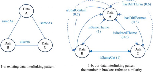
Finally, in our approach, dataset interlinking of LGD is represented by a directed edge associated with an exact relation predicate and a quantitative similarity. The difference of the dataset interlinking created by the proposed approach from that of existing methods is shown in Figure 1. The proposed approach transforms the existing simple and qualitative geospatial dataset interlinking (Figure 1(a)) to complete and quantitative interlinking (Figure 1(b)).

Figure 1. Comparison of existing methods and our approach of geospatial dataset interlinking.

2.2. Geospatial data interlinking types and predicates

According to the roles in data discovery, the characteristics of geospatial data can be divided into two types: intrinsic and morphologic characteristics. Intrinsic characteristics refer to the basic ‘what, where, when’ triple features of geospatial data, namely, data content and spatial and temporal coverage. These characteristics make geospatial data distinguishable from one another. Morphologic characteristics represent the structural and shape features of geospatial data, such as data type, format, and spatiotemporal precision. Morphologic characteristics can be transformed with more or less information loss without affecting the nature of geospatial data.

The detailed intrinsic and morphologic characteristics of geospatial data are shown in Table 1. Each data characteristic on different levels in Table 1 represents one unique data interlinking type. Thus, multidimensional and hierarchical geospatial data interlinking types are formed in consideration of a single data characteristic or a combination of multiple data characteristics.

Table 1. Geospatial data characteristics and corresponding data interlinking types.

Overall characteristic	Compound characteristics	Compound characteristics	Elementary characteristics
Geospatial data overall characteristic (A)	Intrinsic characteristic (B1)	Content (C1)	Theme (D1)
			Category (D2)
		Spatial coverage (C2)	Spatial topology (D3)
		Temporal coverage (C3)	Temporal topology (D4)
	Morphologic characteristic (B2)	Spatiotemporal Precision (C4)	Spatial precision (D5)
			Temporal granularity (D6)
		Structure (C5)	Type (D7)
			Format (D8)

The relational instances of each data interlinking type are shown in Table 2. These relational instances can be regarded as predicates of RDF to exactly describe the data interlinking types of LGD. Only the different relational instance of all morphologic data interlinking types is retained because morphologic characteristics are transformable, whereas such a relation instance is irrelevant for intrinsic data interlinking types. The properties of each predicate (see Table 2) are further defined to implement the reasoning of data interlinking relation.

Table 2. Data interlinking relation instances, predicates, and properties: S refers to symmetry, T means transitivity, and I indicates inverse.

Data characteristic	Data characteristic instances	Interlinking predicates	Properties of predicates
Theme	Same theme	isSameTheme	S, T
	Similar theme	isRelatedTheme	S
Category	Same category	isSameCat	S, T
	Parent category	isParentCat	T, I (isChildCat)
	Child category	isChildCat	T, I (isParentCat)
	Sibling category	isSiblingCat	S, T
Spatial topology	Spatial equal	isSpatEqual	S, T
	Spatial contain	isSpatContain	T, I (isSpatWithin)
	Spatial within	isSpatWithin	T, I (isSpatContain)
	Spatial overlap	isSpatOverlap	S
	Spatial touch	isSpatTouch	S
Temporal topology	Temporal equal	isTempEqual	S, T
	Temporal contain	isTempContain	T, I (isTempWithin)
	Temporal within	isTempWithin	T, I (isTempContain)
	Temporal overlap	isTempOverlap	S
	Temporal touch	isTempTouch	S
Spatial precision	Same spatial precision	hasSameSPrecise	S, T
	Different spatial precision	hasDiffSPrecise	S
Temporal granularity	Same temporal granularity	hasSameTGran	S, T
	Different temporal granularity	hasDiffTGran	S
Type	Same type	hasSameType	S, T
	Different type	hasDiffType	S
Format	Same format	hasSameFormat	S, T
	Different format	hasDiffFormat	S

2.3. Similarity calculation for geospatial data interlinking

2.3.1. Theme similarity

Theme similarity refers to the correlation degree of content topics between two geospatial datasets. For most geospatial metadata, data topic is usually included in the title, keyword, and abstract elements (referred to as ‘topic–element’ hereafter). Theme similarity is calculated with the equation below. Hereafter, the intended interlinking datasets are A and B, and the interlinking direction is from dataset A to dataset B.(1) where is the theme similarity, refers to the number of topic words in the topic–element of dataset B, is the number of matched topic words in dataset A, and is the corresponding weight of topic–element for theme similarity. The weights of title, keyword, and abstract topic–elements are set to 0.529, 0.309, and 0.162, respectively, by using the analytic hierarchy process (AHP) method (Saaty 1990).

2.3.2. Category similarity

Given that datasets A and B separately contain categories and in the same classification system and have the closest parent category , the category similarity calculation can be defined as Equation (2) (Wu and Palmer 1994).(2) where is the number of edges from to , is the number of edges from to , and is the number of edges from to the category root node.

If datasets A and B belong to different category systems, their categories must be consistently converted to the designated category system. Global Change Master Directory (GCMD 2015) is considered the unified topic category in this work. If datasets A and B have several categories, then category similarity is calculated with Equation (3).(3)

where is the category similarity of the category of dataset A and the category of dataset B. m and n are the total number of categories of datasets A and B, respectively.

2.3.3. Spatial topology similarity

The spatial coverage of a geospatial dataset is usually expressed by the minimum enclosing rectangle of the dataset. Therefore, six polygon–polygon relations are selected to represent the spatial topology interlinking of geospatial data. These six are ‘equal,’ ‘contain,’ ‘within,’ ‘overlap,’ ‘touch,’ and ‘disjoint.’ Furthermore, the disjoint topology relation is removed from the spatial topology interlinking because its value for LGD is limited and it substantially increases the number of such links (Yuan et al. 2013).

For the same spatial topology relation, the correlation degree of geospatial data may differ from the variation in their spatial distance or overlapping area. Thus, spatial topology similarity calculation needs to further consider such a quantitative difference based on topology relations. The detailed spatial topology similarity calculation is as follows:(4) where is the spatial topology similarity and and are the basic similarity of each spatial topology and the distance similarity, respectively. and are the corresponding weights of and , which are set to 0.875 and 0.125, respectively, with the AHP method. The values of of each spatial topology are 1.00, 0.85, 0.65, 0.60, and 0.25based on experts’ experiences, when the spatial topology relations are ‘equal,’ ‘contain,’ ‘within,’ ‘overlap,’ and ‘touch,’ respectively. is calculated with Equation (5).(5)

where and are the spatial coverage polygon areas of datasets A and B; is the overlapping area of datasets A and B; is the perimeter of dataset B; and is the length of the intersection of datasets A and B.

2.3.4. Temporal topology similarity

Temporal topology is the relationship between geo-objects in time. This type of topology indicates the time of dataset A before, after, or simultaneously as dataset B. The two forms of time are instant and interval (Hobbs and Pan 2004). Instant denotes a moment in time, whereas interval refers to a continuous period, which includes start and end instances (Hou et al. 2015). Instant and interval forms are relative and we are always able to transform the instant time to the interval time through time-scale conversion. Therefore, similar to the calculation of spatial topology, five relations of interval–interval are selected to represent the temporal topology of geospatial datasets. These five are ‘equal,’ ‘contain,’ ‘within,’ ‘overlap,’ and ‘touch.’

Similar to that of spatial topology, the degree of temporal correlation may also differ because of the variation in temporal distance in the same temporal topology. In addition, users prefer to use new datasets. Thus, the temporal sequence must be further considered based on temporal basic and distance similarities when calculating the similarity temporal topology. The detailed temporal topology similarity calculation is defined as Equation (6).(6) where and are the basic similarity of each temporal topology and the distance similarity, respectively; and are the corresponding weights of and , respectively; and is the weight of the temporal sequence, which further determines the role of time order for temporal topology similarity. , , and have the same values as , , and . For overlap and touch temporal topology, according to experts’ experiences, is set to 1.00 and 0.875 when the time order is before and after, respectively. Since time order is irrelevant for the equal, contain, and within temporal topology, their is always equal to 1. is calculated with Equation (7).(7) where and are the time distances of datasets A and B at the same time scale, and is their overlapping time distance, and and denote the middle time of datasets A and B, respectively.

2.3.5. Spatial precision similarity

Spatial precision generally includes spatial scale (for vector data) or resolution (for raster data) and granularity factors. Spatial scale or resolution reflects the location precision and detailed degree of ground features, and spatial granularity indicates the fine level of a region partition. Thus, spatial precision similarity is calculated with the following equation.(8) where is the spatial precision similarity; and are the spatial scale and resolution and granularity similarities, respectively; and and are the corresponding weights of and , which are set to 0.5 based on the AHP method.

and are measured mainly based on the conversion difficulty degree. Spatial scale and resolution conversions are usually implemented through upscaling and downscaling methods. Many spatial upscaling and downscaling methods (Crane and Hewitson 1998; Hong, Hendrickx, and Borchers 2009; Uvin 1995; Zhang et al. 2012) demonstrate that the upscaling conversion of geographic data is considerably easier than downscaling conversion. Therefore, when the spatial scales or resolutions of two datasets are the same, their similarity is equal to 1; when their spatial scales or resolutions require upscaling and downscaling conversion, their similarities are set to 0.875 and 0.125, respectively, with the AHP method.

Spatial granularity can also be converted with varying degrees of difficulty and rates of information loss. The conversion from fine to coarse granularity is easier than that from coarse to fine. The latter usually requires the support of domain models. Thus, spatial granularities are set to 1.000, 0.875, and 0.125 when the spatial granularities of datasets A and B are the same, fine to coarse, and coarse to fine, respectively.

2.3.6. Temporal granularity similarity

Temporal granularity refers to the time precision of geospatial data. For example, the granularity of precipitation data could be in hours, days, months, years, or average years. Similar to spatial granularity, temporal granularity can also be converted through upscaling and downscaling methods. Temporal upscaling conversion can be implemented by addition or averaging operations. Temporal downscaling conversion usually requires a specific professional model and is thus considerably more complex than upscaling conversion (Lombardo, Volpia, and Koutsoyiannis 2012; Yang, Bárdossy, and Caspary 2010). Thus, temporal granularity similarities are also set to 1.000, 0.875, and 0.125 when the temporal granularities of datasets A and B are the same, fine to coarse, and coarse to fine, respectively.

2.3.7. Data type similarity

Data type similarity is determined by the data type transformation kind. Geospatial data are generally categorized as sensible and latent. The former refers to tangible geospatial map layers, which contain vector and raster sub-data types. The latter refers to non-map layer data, but this type of data contains geographic location information, such as coordinates, administrative codes, and place names. Latent spatial data usually include tables (such as population statistical data on a county level) and plain text (such as air pollution automatic monitoring data) as subtypes. The transformations of these four data types are of three kinds, namely, same subtype transformation, same main-type transformation, and completely different transformation.

According to experts’ experiences, when two datasets have similar subtypes, data type similarity is set to 1. When two datasets have the same main types, the similarity is set to 0.8–0.9. Similarity is set to 0.45–0.75 for the completely different transformation type. In addition, users prefer sensible spatial data to latent spatial data, editable vector data to raster data, and standardized table data to text data in geospatial discovery. Therefore, the similarities of all 16 instances of the 3 data type transformations mentioned above are further refined. The detailed instances of the data type transformations and their similarities are shown in Table 3.

Table 3. Data type transformation instances and their similarities.

Transformation kind	Transformation instance	Data type similarity	Transformation kind	Transformation instance	Data type similarity
Same subtype		1	Total different type		0.75
		1			0.7
		1			0.75
		1			0.7
Same main type		0.9			0.6
		0.8			0.5
		0.8			0.55
		0.9			0.45

2.3.8. Data format similarity

Data format similarity depends on the degree of conversion difficulty. The similarity is high when the format conversion is easy. The relations of the formats of geospatial datasets are categorized into three: same-data formats, same-family formats, and different-family formats. Same-data formats do not require conversion. Thus, the similarity is set to 1. Same-family formats are easily converted by using existing tools. For example, ArcGIS family includes ArcInfo coverage, interchange file, and Shapefile formats, which can be easily converted using ArcGIS conversion tools. Therefore, the similarity of these formats is set to 0.85 according to experts’ experiences. The degree of conversion difficulty in different-family formats is measured according to the openness of these formats.

Data format openness can be evaluated with sustainability factors, which include disclosure, documentation, adoption, and external dependency of formats (Arms and Fleischhauer 2015). The qualitative openness of each sustainability factor of most geospatial data formats can be obtained from digital formats in the Library of Congress of the United States. Qualitative openness is categorized into three classes, as shown in Table 4.

Table 4. Openness classification of data format sustainability factors.

Factors	Openness
	High (0.85)	Medium (0.65)	Low (0.35)
Disclosure	Full open	Part open	closed
Adoption	Wide use	Local use	Seldom use
Self-document integration	Intact	Basic complete	None or unreadable
External dependency	Independent	Dependent	Heavily dependent

The openness values are set to 0.85, 0.65, and 0.35 when the openness class is high, medium, and low, respectively, according to experts’ experiences. The lowest openness factor of two datasets is assumed to mainly influence the degree of conversion difficulty. Therefore, data format similarity can be calculated with Equation (9).(9) where is the data format similarity and and are the openness values of the sustainability factor of datasets A and B, respectively.

2.3.9. Compound similarities and overall similarity

Based on these elementary similarities, all compound similarities and overall similarity can be calculated with the AHP method. The detailed calculation is defined in Equation (10).(10) where is the target compound similarity or overall similarity; and denote the similarity and weight of the subtype of the target data interlinking type; and is the number of subtypes. is determined by using the domain expert scoring method of AHP (see Table 5).

Table 5. Weights for compound similarities and overall similarity calculation.

Type element	Type element	Local/global weight	Type element	Local weight	Global weight	Type element	Local weight	Global weight
A	B1	0.875	C1	0.535	0.4681	D1	0.875	0.4096
						D2	0.125	0.0585
			C2	0.344	0.3011	D3	1	0.3011
			C3	0.121	0.1058	D4	1	0.1058
	B2	0.125	C4	0.833	0.1041	D5	0.667	0.0694
						D6	0.333	0.0347
			C5	0.167	0.0209	D7	0.750	0.0157
						D8	0.250	0.0052
Sum	/	1	/	/	1	/	/	1

3. Case study

3.1. Data sources

Three platforms of Chinese National Scientific and Technology Infrastructure (NSTI), namely, National Earth System Scientific Data Sharing Network (NSTI-GEO, http://www.geodata.cn), Chinese Meteorological Data Network (NSTI-CMA, http://data.cma.cn/), and National Population and Health Scientific Data Sharing Platform (NSTI-PH, http://www.ncmi.cn), were used as the data resources in the case study.

The datasets of NSTI-GEO cover many fields, such as land surface, terrestrial hydrosphere, cryosphere, paleoclimate, solid Earth, Sun–Earth interactions, atmosphere, oceans, and human dimensions. The platform also contains typical regional datasets, such as Polar, Qinghai–Tibet Plateau, Loess Plateau, Yangtze Delta, Yellow River Delta, China Northeastern Plain, and China Southwestern Mountain. NSTI-CMA mainly provides long-term series and real-time meteorological data services, including ground- and upper-air monitoring, satellite remote sensing, weather radar probing, numerical prediction, and modeling datasets. NSTI-PH includes datasets on basic medicine, clinical medicine, public health, traditional Chinese medicine, pharmacy, population, and reproductive health. These platforms publish their data through different metadata standards. Their datasets are simply linked in an intra-platform by data categories. However, no inter-platform data interlinking is available for these platforms. So it is difficult to provide one-stop dataset services for cross-disciplinary researches, such as ‘How will climate change affect infection rate of dengue fever in China?’

Therefore, dataset interlinking was implemented in two levels using the proposed method: intra-data interlinking of NSTI-GEO and inter-data interlinking of NSTI-GEO with NSTI-CMA and NSTI-PH. To reduce the calculation amount in the experiment, we only selected 40 datasets from NSTI-GEO whose themes are related to meteorology, population, and health, such as administrative boundary, land use/cover, soil, environmental pollution, natural hazard, population, and socioeconomics. Twenty datasets on ground monitoring, assimilation meteorology, and meteorological hazard were selected from NSTI-CMA, and 20 datasets on infectious disease, population, and reproductive health, which have evident spatiotemporal information, were selected from NSTI-PH.

3.2. Data interlinking process

The overall workflow of geospatial data interlinking includes four steps, as shown in Figure 2.

Figure 2. The overall workflow of geospatial data interlinking.

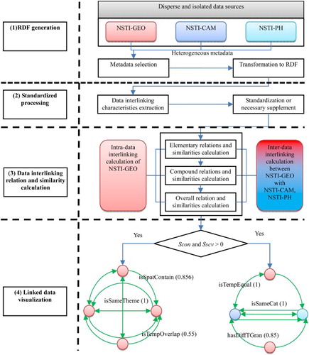
3.2.1. RDF generation

According to the designated data categories, 40, 20, and 20 metadata were selected from NSTI-GEO, NSTI-CAM, and NSTI-PH, respectively. These metadata were manually transformed to RDF because such metadata are heterogeneous. The URI of each RDF record is composed of a site identifier and an existing interior metadata identifier.

3.2.2. Linked characteristics extraction and standardization

As shown in Table 1, data interlinking characteristics were extracted and standardized or necessarily supplemented; for instance, data category conversion to GCMD category, data format supplement, etc.

3.2.3. Data interlinking relations and similarity calculation

The data interlinking relations and corresponding similarities in two levels were calculated using the approach elaborated in Section 2.3. The first level pertains to the intra-links among the datasets of NSTI-GEO, and the second level includes the interlinks between NSTI-GEO with NSTI-CAM and NSTI-PH.

3.2.4. Linked data visualization

The graph of directed edge with textual relation predicates, and numerical similarities was used to present the data interlinking network according to the calculation results of step 3. Different LGD interlinking network graphs (LGDNG) were established according to interlinking types by employing this method. In terms of geospatial data interlinking, if the content and spatial coverage of two datasets are completely unrelated, such interlinking is illogical. Therefore, when the similarities of data content or spatial coverage are equal to 0, all links of two datasets are invalid and will be removed from LGDNG.

3.3. Results

The experimental geospatial datasets were interlinked in two levels (intra-links among NSTI-GEO datasets and interlinks between NSTI-GEO with NSTI-CAM and NSTI-PH), according to the workflow described above. These data links contain elementary links of data theme, category, spatial topology, temporal topology, spatial precision, temporal granularity, data type, and format, as well as compound links of data content, spatiotemporal precision, data structure, data intrinsic characteristic, and morphologic characteristic, and overall data characteristic links.

For 40 datasets of NSTI-GEO, we totally calculated 10,920 intra-links of 780 dataset-pairs (each dataset-pair has 14 link types as shown in Table 1). And we found that 6790 intra-links of 485 dataset-pairs are invalid because their or is equal to 0. While for interlinks of NSTI-GEO with NSTI-CAM and NSTI-PH, there are 14,406 invalid interlinks of 1029 dataset-pairs in the total 22,400 interlinks of 1600 dataset-pairs. The results show that the average, maximum, and minimum overall similarities are 0.46, 0.98, and 0.217, respectively, in the valid intra-links and interlinks.

The top five dataset intra-links of NSTI-GEO, and interlinks of NSTI-GEO with NSTI-CAM and NSTI-PH are listed in Table 6 according to the overall similarities. In Table 6, A, B1, B2, C1, C2, C3, C4, D1, D2, D3, D4, D5, D6, D7, and D8 represent the interlinking types whose meanings are listed in Table 1, and we do not show C1, C2, C3, and C4 because of the limited space. Textual descriptions of Table 6 are data interlinking predicates and the numbers in brackets are the data similarities. From the results, we can get all links of each dataset, and further form LGDNG of each dataset with different data interlinking types. With such graph, users can easily discover the most relevant datasets they want. For example, there are 23 datasets having valid intra-links with ‘GEO1: China 1: 4,000,000 Basic Geospatial Dataset (1970s–1990s).’ Table 7 shows the top five dataset (GEO2, GEO3, GEO4, GEO5, and GEO36) intra-links with GEO1 ordered by their overall similarities. Figure 3 shows LGDNG of GEO1 with GEO2, GEO3, GEO4, GEO5, and GEO36.

Figure 3. LGD network graph of GEO1 with GEO2, GEO3, GEO4, GEO5, and GEO36.

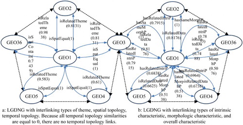
Table 6. The top five intra-links of NSTI-GEO and interlinks of NSTI-GEO with NSTI-CAM and NSTI-PH ordered by the overall data similarities.

Dataset A	Dataset B	D1	D2	D3	D4	D5	D6	D7	D8	B1	B2	A
Intra-links of NSTI-GEO datasets
GEO6: China 1KM Land Use/Cover Fusion Grid Dataset (2000)	GEO8: China 1KM Land Use Grid Dataset (2000)	isRelatedTheme (0.9558)	isSameCategory (1)	isSpatEqual (1)	isTempEqual (1)	hasSameSPrecise (1)	hasSameTGran (1)	hasSameType (1)	hasDiffFormat (0.65)	hasRelatedIntriP (0.9793)	hasRelatedMorphP (0.9854)	isRelatedData (0.9801)
GEO10: China Monthly Precipitation Simulation Grid Dataset (1950–2006)	GEO13: China Multi-Year Average Precipitation Distribution Vector Map (1980–1996)	isSameTheme (1)	isSameCategory (1)	isSpatEqual (1)	isTempContain (0.7788)	hasDiffSPrecise (0.875)	hasDiffTGran (0.875)	hasSameType (1)	hasDiffFormat (0.65)	hasRelatedIntriP (0.9732)	hasRelatedMorphP (0.8813)	isRelatedData (0.9617)
GEO29: China Annually Droughts & Floods Distribution Vector Map (1571–1670)	GEO30: China Annually Droughts & Floods Distribution Vector Map (1671–1770)	isSameTheme (1)	isSameCategory (1)	isSpatEqual (1)	isTempTouch (0.22)	hasSameSPrecise (1)	hasSameTGran (1)	hasSameType (1)	hasSameFormat (1)	hasRelatedIntriP (0.9056)	hasSameMorphP (1)	isRelatedData (0.9174)
GEO7: China 1KM Land Use Grid Dataset (1995)	GEO8: China 1KM Land Use Grid Dataset (2000)	isSameTheme (1)	isSameCategory (1)	isSpatEqual (1)	isTempDisjoint (0)	hasSameSPrecise (1)	hasSameTGran (1)	hasSameType (1)	hasSameFormat (1)	hasRelatedIntriP (0.879)	hasSameMorphP (1)	isRelatedData (0.8941)
GEO2: China 1:4,000,000 Administrative Boundary Dataset on County Level (2005)	GEO3: China 1:4,000,000 Administrative Boundary Dataset on County Level (2000)	isSameTheme (1)	isSameCategory (1)	isSpatEqual (1)	isTempDisjoint (0)	hasSameSPrecise (1)	hasSameTGran (1)	hasSameType (1)	hasSameFormat (1)	hasRelatedIntriP (0.879)	hasSameMorph (1)	isRelatedData (0.8941)
Interlinks of NSTI-GEO and NSTI-CAM datasets
GEO10: China Monthly Precipitation Simulation Grid Dataset (1950-2006)	CAM8: China Monthly Ground Precipitation Grid Dataset (1961-2015)	isRelatedTheme (0.8455)	isSameCategory (1)	isSpatEqual (1)	isTempOverlap (0.6277)	hasDiffSPrecise (0.875)	hasSameTGran (1)	hasSameType (1)	hasDiffFormat (0.65)	hasRelatedIntriP (0.8826)	hasRelatedMorphP (0.9159)	isRelatedData (0.8868)
GEO29: China Annually Droughts and floods Distribution Vector Map (1571–1670)	CAM13: China Annually Droughts and Floods Level Vector Map (1470–2000)	isSameTheme (1)	isSameCategory (1)	isSpatEqual (1)	isTempWithin (0.5923)	hasDiffSPrecise (0.125)	hasSameTGran (1)	hasDiffType (0.45)	hasDiffFormat (0.85)	hasRelatedIntriP (0.9507)	hasRelatedMorphP (0.4387)	isRelatedData (0.8868)
GEO30: China Annually Droughts and floods Distribution Vector Map (1671-1770)	CAM13: China Annually Droughts and Floods Level Vector Map (1470-2000)	isSameTheme (1)	isSameCategory (1)	isSpatEqual (1)	isTempWithin (0.5923)	hasDiffSPrecise (0.125)	hasSameTGran (1)	hasDiffType (0.45)	hasDiffFormat (0.85)	hasRelatedIntriP (0.9507)	hasRelatedMorphP (0.4387)	isRelatedData (0.8867)
GEO11: China Monthly Temperature Simulation Grid Dataset (1950–2006)	CAM6: China Monthly Ground Temperature Grid Dataset (1961–2015)	isRelatedTheme (0.8455)	isSiblingCategory (0.6667)	isSpatEqual (1)	isTempOverlap (0.6277)	hasDiffSPrecise (0.875)	hasSameTGran (1)	hasSameType (1)	hasDiffFormat (0.65)	hasRelatedIntriP (0.8603)	hasRelatedMorphP (0.9159)	isRelatedData (0.8673)
GEO9: China 3 Hourly Meteorology Parameter Assimilation Grid Dataset (1979–2012)	CAM5: China Daily Ground Temperature Grid Dataset (1961–2015)	isRelatedTheme (0.8455)	isSiblingCategory (0.6667)	isSpatEqual (1)	isTempWithin (0.6446)	hasDifferSPrecise (0.875)	hasDiffTGran (0.875)	hasDiffType (0.7)	hasDiffFormat (0.65)	hasRelatedIntriP (0.8624)	hasRelatedMorphP (0.8437)	isRelatedData (0.86)
Interlinks of NSTI-GEO and NSTI-PH datasets
GEO16: China 1KM Population Distribution Grid Dataset (2005, 2010)	PH2: China Illiteracy Population aged 15 and over Statistical Dataset on Provincial Level (2010)	isRelatedTheme (0.686)	isSiblingCategory (0.6667)	isSpatEqual (1)	isTempEqual (1)	hasDiffSPrecise (0.875)	hasSameTGran (1)	hasDiffType (0.6)	hasDiffFormat (0.65)	hasRelatedIntriP (0.8307)	hasRelatedMorphP (0.8658)	isRelatedData (0.8351)
GEO16: China 1KM Population Distribution Grid Dataset (2005, 2010)	PH3: China Population by Gender and Nation Statistical Dataset on Provincial Level (2010)	isRelatedTheme (0.686)	isSiblingCategory (0.6667)	isSpatEqual (1)	isTempEqual (1)	hasDiffSPrecise (0.875)	hasSameTGran (1)	hasDiffType (0.6)	hasDiffFormat (0.65)	hasRelatedIntriP (0.8307)	hasRelatedMorphP (0.8658)	isRelatedData (0.8351)
GEO17: China Annually Population Statistical Dataset on Province Level (2002–2008)	PH6: China Annually Birth, Death and Natural Growth Rate of Population Dataset (1949–2011)	isRelatedTheme (0.688)	isParentCategory (0.8333)	isSpatEqual (1)	isTempWithin (0.5826)	hasDiffSPrecise (0.875)	hasSameTGran (1)	hasSameType (1)	hasSameFormat (1)	hasRelatedIntriP (0.7923)	hasRelatedMorphP (0.9305)	isRelatedData (0.8096)
GEO17: China Annually Population Statistical Dataset on Province Level (2002-2008)	PH7: China Annually Age structure and Dependency Ratio of Population Dataset (1953-2011)	isRelatedTheme (0.686)	isParentCategory (0.8333)	isSpatEqual (1)	isTempWithin (0.5836)	hasDiffSPrecise (0.875)	hasSameTGran (1)	hasSameType (1)	hasSameFormat (1)	hasRelatedIntriP (0.7915)	hasRelatedMorphP (0.9305)	isRelatedData (0.8089)
GEO16: China 1KM Population Distribution Grid Dataset (2005, 2010)	PH7: China Annually Age structure and Dependency Ratio of Population Dataset (1953–2011)	isRelatedTheme (0.686)	isSiblingCategory (0.6667)	isSpatEqual (1)	isTempWithin (0.5709)	hasDiffSPrecise (0.875)	hasSameTGran (1)	hasDiffType (0.6)	hasDiffFormat (0.65)	hasRelatedIntriP (0.7788)	hasRelatedMorphP (0.8658)	isRelatedData (0.7899)

Table 7. The top five intra-links with ‘GEO1: China 1:4,000,000 Basic Geospatial Dataset (1970s–1990s)’ in NSTI-GEO ordered by the overall data similarity (Basic geospatial data include boundary, topography, geomorphology, river, transportation, soil, land cover data, etc.).

Interlinking Dataset	D1	D2	D3	D4	D5	D6	D7	D8	B1	B2	A
GEO2: China 1:4,000,000 Administrative Boundary Dataset on County Level (2005)	isRelatedTheme (0.8131)	isSameCat (1)	isSpatEqual (1)	isTempDis joint (0)	hasSameSPrecise (1)	hasSameTGran (1)	hasSameType (1)	hasSameFormat (1)	hasRelatedIntriP (0.7915)	hasSameMorphP (1)	isRelatedData (0.8176)
GEO3: China 1:4,000,000 Administrative Boundary Dataset on County Level (2000)	isRelatedTheme (0.8131)	isSameCat (1)	isSpatEqual (1)	isTempDisjoint (0)	hasSameSPrecise (1)	hasSameTGran (1)	hasSameType (1)	hasSameFormat (1)	hasRelatedIntriP (0.7915)	hasSameMorphP (1)	isRelatedData (0.8176)
GEO36: Taihu Basin of China 1:250,000 Basic Geospatial Dataset (2002)	isRelatedTheme (0.9838)	isSameCat (1)	isSpatContain (0.7439)	isTempDisjoint (0)	hasDiffSPrecise (0.125)	hasSameTGran (1)	hasSameType (1)	hasRelatedFormat (0.85)	hasRelatedIntriP (0.7833)	hasRelatedMorphP (0.5076)	isRelatedData (0.7488)
GEO4: China 1:1,000,000 Main River Spatial Dataset (2002)	isRelatedTheme (0.61)	isSameCat (1)	isSpatEqual (1)	isTempDisjoint (0)	hasDiffSPrecise (0.125)	hasSameTGran (1)	hasSameType (1)	hasSameFormat (1)	hasRelatedIntriP (0.6964)	hasRelatedMorphP (0.5138)	isRelatedData (0.6736)
GEO5: China 1:250,000 Lake with Area Above 1 km^2 Dataset (2005–2006)	isRelatedTheme (0.583)	isSameCat (1)	isSpatEqual (1)	isTempDisjoint (0)	hasDiffSPrecise (0.125)	hasSameTGran (1)	hasSameType (1)	hasSameFormat (1)	hasRelatedIntriP (0.6838)	hasRelatedMorphP (0.5138)	isRelatedData (0.6625)

4. Discussion

4.1. Data similarity threshold value and interlinking reliability

Geospatial data interlinking amount is significantly affected by the similarity threshold value. The amount of data interlinking is high when the similarity threshold value is small. Table 8 shows the increasing conditions of the number of intra- and interlinks with a similarity threshold value from 0.8 to 0.4. Table 8 indicates that the amount of data interlinking increases when the similarity threshold value decreases, and different data similarities exhibit varying growth rates of the data interlinking amount.

Table 8. The amount of data interlinking with different data similarities threshold values.

Data similarity threshold value	Overall similarity			Content similarity			Spatial similarity			Temporal similarity
	0.8	0.6	0.4	0.8	0.6	0.4	0.8	0.6	0.4	0.8	0.6	0.4
Intra-links of NSTI-GEO	12	33	398	19	28	34	435	740	749	31	157	368
Interlinks of NSTI-GEO and NSTI-CAM	17	75	394	29	68	86	512	574	794	14	193	514
Interlinks of NSTI-GEO and NSTI-PH	4	18	402	0	13	19	600	600	800	23	155	266

Although the similarity threshold value is crucial to data interlinking, selecting a suitable value that balances the quality and construction efficiency of LGD is difficult. Complex network centrality theory will be adopted in future work to measure the importance of each node of data links, remove data links that have weak associations and low values, and improve the quality of LGD.

4.2. Selection of data characteristic factors and interlinking types

Eight major characteristics, namely, data theme, category, spatial topology, temporal topology, spatial precision, temporal granularity, data type, and format, were selected as the basis of determining interlinking types. Such interlinking types can basically meet the requirements of fine data discovery. However, other characteristics could be further considered as interlinking factors, such as data spatial datum (coordinate and elevation reference system), data provenance, and coding and classification system of data attribute fields. Especially, data provenance records data sources, data process and management methods, models, and agents (organizations or individuals) (Yuan et al. 2013). Users can trace the original or derivative datasets and understand the production process and quality of datasets through data provenance links. Therefore, data provenance interlinking needs to be urgently considered in the further work.

4.3. Data interlinking precision and calculation efficiency

Data interlinking precision is affected by metadata quality and the calculation algorithm. Metadata quality mainly depends on data contributors. NSTI-GEO, NSTI-CAM, and NSTI-PH are handled by different institutes and adopt different metadata standards. Thus, the results of their metadata qualities vary. Heterogeneous metadata must be harmonized, and preprocessing, such as topic category harmonization, data theme word processing, and extracting the minimum enclosing rectangle of datasets, must be carried out to meet data interlinking calculation requirements. However, preprocessing reduces interlinking precision. For example, in spatial topology similarity calculation, the overlapping area of two datasets is always overrated because the actual boundary coordinates of the datasets are substituted by the coordinates of the minimum enclosing rectangle. Preprocessing is also considerably time consuming. Therefore, automatic preprocessing, such as metadata topic category harmonization based on machine learning (Hu et al. 2015), must be further studied. Algorithms for data similarity calculation can be further optimized in the future to improve the precision of data interlinking. For instance, spatial precision, temporal granularity, data type, and format similarities can be determined according to the information loss rates of their conversions.

The calculation efficiency of data interlinking construction is another issue to be studied in our next research. The results of the case study indicated that the amount of intra-link calculation is , whereas the amount of interlink calculation is , where is the number of interlinking types, is the number of NSTI-GEO datasets, is the number of NSTI-CAM datasets, and is the number of NSTI-PH datasets. Even in our case study, , , , and , which are pretty larger numbers for data interlinking calculation. Therefore, high-performance calculation methods should be considered from multiple aspects. These methods may include adopting distributed and parallel calculation, setting a reasonable threshold value to remove invalid calculations, and maximizing data relation reasoning to avoid repeated calculations. The process to increase the efficiency of updating data interlinking when a new dataset is added should also be studied.

4.4. Applications of multidimensional and quantitative LGD approach

Traditional RDF-based representation of Linked Data includes the URI, and interlinking type as well as corresponding resources. It does not represent the quantified association degree of each interlinking. Therefore, we need consider adding this association degree or data similarity value as a numerical attribute of each interlinking in RDF.

The proposed approach can be used to establish intra-links and interlinks in the case study of NSTI-GEO, NSTI-CAM, and NSTI-PH as well as in all other scientific data platforms of NSTI, such as China Earthquake Data Center (http://data.earthquake.cn/), National Forest Data Center (http://www.cfsdc.org/), and National Agriculture Data Sharing Center (http://www.agridata.cn/). Meanwhile, it can be expanded to establish data interlinking with external open data-sharing platforms or portals, such as GCMD (http://gcmd.nasa.gov) and Group on Earth Observations System of Systems Portal (http://www.geoportal.org) that utilize metadata to describe and publish data resources.

The proposed approach can help establish high-quality LGD and may connect different open science and technology resources on various interlinking types, as well as avoid the emerging silos of rapidly expanding data-sharing platforms. It will provide a novel graph-based data discovery way in which users can find good ranking datasets of the same or similar theme, category, spatial and temporal coverage, etc., without providing professional key words. With assistant tools supporting, the proposed approach will extremely promote the development of spatial data infrastructure (SDI), LGD, and its applications.

5. Conclusions

A multidimensional and quantitative data interlinking approach was proposed for LGD. In the approach, the data interlinking types are determined based on geospatial data characteristics and their roles in data discovery, which include two aspects (intrinsic and morphologic characteristic links) and three levels (elementary, compound, and overall characteristic links). These elementary links contain data theme, category, spatial topology, temporal topology, spatial precision, temporal granularity, data type, and format links, which are gradually combined to form compound and overall characteristic links. Each data interlinking type adopts one specific predicate to indicate the actual relationship of datasets and uses the similarity of data characteristics to quantitatively represent the correlation degree. Thus, dataset interlinking can be expressed using a directed edge associated with an exact relation predicate and a quantitative similarity. Through such data interlinking, users can determine the existing relations of geospatial datasets and the closeness of these relations.

As illustrated in the case study, this research effectively contributes to the establishment of the high-quality and trusted LGD to prevent the formation of the emerging silos of rapidly expanding data-sharing platforms and promote the accurate discovery, recommendation, and extensive sharing of open geospatial data. And also it can integrate multi-source, heterogeneous, and distributed datasets, and provide a one-stop dataset service for cross-disciplinary, comprehensive researches.

Future research will focus on expanding data interlinking factors, optimizing algorithms on data similarity calculation, evaluating the importance of data interlinking nodes using complex network centrality theory, improving the efficiency of LGD establishment, and designing the mechanism and method of updating LGD. Combining GeoSPARQL (OGC 2012) with our approach to improve the efficiency and accuracy of LGD querying is another topic in our future research. Automatic tools to preprocess different standards of metadata will also be developed according to the requirements of data interlinking calculation. Intra-, inter-, and external LGD will be established for all scientific data-sharing platforms of NSTI using the proposed method and existing RDF publishing tools.

Disclosure statement

No potential conflict of interest was reported by the authors.

ORCID

Jia Song http://orcid.org/0000-0002-9051-1925

Additional information

Funding

This work was supported by the National Natural Science Foundation of China [grant number 41371381], [grant number 41431177]; Natural Science Research Program of Jiangsu [grant number 14KJA170001]; National Special Program on Basic Works for Science and Technology of China [grant number 2013FY110900]; National Key Technology Innovation Project for Water Pollution Control and Remediation [grant number 2013ZX07103006]; National Basic Research Program of China [grant number 2015CB954102]; GuiZhou Welfare and Basic Geological Research Program of China [grant number 201423]; China Scholarship Council [grant number 201504910358].

Notes

1 DBPedia: http://wiki.dbpedia.org.

2 GeoNames: http://www.geonames.org.

3 GDAM: http://www.gadm.org.

4 D2R Server: http://d2rq.org/d2r-server.

5 Virtuoso Universal Server: http://semantic.ckan.net.

6 Talis Platform: https://www.w3.org/2001/sw/wiki/TalisPlatform.

7 Pubby: https://www.w3.org/2001/sw/wiki/Pubby.

8 Triplify: http://semanticweb.org/wiki/Triplify.html.

9 http://www.freebase.com/.

References

- Arms, C., and C. Fleischhauer. 2005. “Digital Formats: Factors for Sustainability, Functionality, and Quality.” Archiving Conference, Archiving 2005 Final Program and Proceedings, 222–227. http://memory.loc.gov/ammem/techdocs/digform/Formats_IST05_paper.pdf.
- Atemezing, G., O. Corcho, D. Garijo, J. Mora, M. Poveda-Villalón, P. Rozas, D. Vila-Suero, and B. Villazón-Terrazas. 2013. “Transforming Meteorological Data into Linked Data.” Semantic Web 4 (3): 285–290. doi:10.3233/SW-120089.
- Auer, S., C. Bizer, G. Kobilarov, J. Lehmann, R. Cyganiak, and Z. Ives. 2007. “DBpedia: A Nucleus for a Web of Open Data.” Lecture Notes in Computer Science (LNCS) 4825: 722–735. doi:10.1007/978-3-540-76298-0_52.
- Auer, S., J. Lehmann, and S. Hellmann. 2009. “LinkedGeoData: Adding a Spatial Dimension to the Web of Data.” Lecture Notes in Computer Science (LNCS) 5823: 731–746. doi:10.1007/978-3-642-04930-9_46.
- Berners-Lee, T. 2006. “Linked Data-Design Issues.” http://www.w3.org/DesignIssues/LinkedData.html.
- Bizer, C., T. Heath, and T. Berners-Lee. 2009. “Linked Data – The Story So Far.” International Journal on Semantic Web and Information Systems 5 (3): 1–22. doi:10.4018/jswis.2009081901.
- Böhm, C., M. Freitag, A. Heise, C. Lehmann, A. Mascher, F. Naumann, V. Ercegovac, M. Hernandez, P. Haase, and M. Schmidt. 2012. “GovWILD: Integrating Open Government Data for Transparency.” Proceedings of the 21st International Conference on World Wide Web, 321–324. Lyon, France, April 16–20. doi:10.1145/2187980.2188039.
- Crane, R. G., and B. C. Hewitson. 1998. “Doubled CO2 Precipitation Changes for the Susquehanna Basin: Down-Scaling from the Genesis General Circulation Model.” International Journal of Climatology 18 (1): 65–76. doi: 10.1002/(SICI)1097-0088(199801)18:1<65::AID-JOC222>3.0.CO;2-9
- Cuan, L. N., Y. M. Shi, G. Y. Li, X. H. Wu, and N. Liu. 2015. “An Algorithm to Generate Data Linkages of Linked Sensor Data.” International Conference on Cyber-Enabled Distributed Computing and Knowledge Discovery (CyberC), 430–433. IEEE, Xi'an, China. September 17–19. doi:10.1109/CyberC.2015.29.
- Ding, L., T. Lebo, J. S. Erickson, D. DiFranzo, G. T. Williams, X. Li, J. Michaelis, A. Graves, J. G. Zheng, and Z. N. Shangguan. 2011. “TWC LOGD: A Portal for Linked Open Government Data Ecosystems.” Web Semantics: Science, Services and Agents on the World Wide Web 9 (3): 325–333. doi:10.1016/j.websem.2011.06.002.
- FGDC (Federal Geographic Data Committee). 1998. “Content Standard for Digital Geospatial Metadata.” FGDC-STD-001-1998. http://www.fgdc.gov/standards/projects/FGDC-standards-projects/metadata/base-metadata/v2_0698.pdf.
- GCMD (Global Change Master Directory). 2015. “GCMD Keywords, Version 8.1.” Greenbelt, MD: Global Change Data Center, Science and Exploration Directorate, Goddard Space Flight Center (GSFC) National Aeronautics and Space Administration (NASA). http://gcmd.nasa.gov/learn/keywords.html.
- Goodwin, J., C. Dolbear, and G. Hart. 2008. “Geographical Linked Data: The Administrative Geography of Great Britain on the Semantic Web.” Transactions in GIS 12 (S1): 19–30. doi:10.1111/j.1467-9671.2008.01133.x.
- Haslhofer, B., and B. Schandl. 2008. “The OAI2LOD Server: Exposing OAI-PMH Metadata as Linked data.” Linked Data on the Web (LDOW2008). Beijing, China, April 22. http://eprints.cs.univie.ac.at/284/1/lodws2008.pdf.
- Heath, T., and C. Bizer. 2011. “Linked Data: Evolving the Web into a Global Data Space.” In Synthesis Lectures on the Semantic web: Theory and Technology, edited by J. Hendler, and F.V. Harmelen. San Rafael, CA: Morgan & Claypool. doi:10.2200/S00334ED1V01Y201102WBE001.
- Hobbs, J. R., and F. Pan. 2004. “An Ontology of Time for the Semantic Web.” ACM Transactions on Asian Language Information Processing(TALIP) 3 (1): 66–85. doi:10.3115/981732.981751.
- Hong, S. H., J. M. H. Hendrickx, and B. Borchers. 2009. “Up-scaling of SEBAL Derived Evapotranspiration Maps from Landsat (30 M) to MODIS (250 M) Scale.” Journal of Hydrology 370 (1–4): 122–138. doi:10.1016/j.jhydrol.2009.03.002.
- Hou, Z. W., Y. Q. Zhu, X. Gao, P. Pan, K. Luo, and D. X. Wang. 2015. “Time-ontology and Its Application in Geodata Retrieval.” Journal of Geo-Information Science 17 (4): 379–390. doi:10.3724/SP.J.1047.2015.00379. (in Chinese).
- Hu, Y. J., K. Janowicz, S. Prasad, and S. Gao. 2015. “Metadata Topic Harmonization and Semantic Search for Linked-Data-driven Geoportals: A Case Study Using ArcGIS Online.” Transactions in GIS 19 (3): 398–416. doi:10.1111/tgis.12151.
- Isele, R., and C. Bizer. 2013. “Active Learning of Expressive Linkage Rules Using Genetic Programming.” Web Semantics: Science, Services and Agents on the World Wide Web 23: 2–15. doi:10.1016/j.websem.2013.06.001.
- Isele, R., A. Jentzsch, and C. Bizer. 2011. “Efficient Multidimensional Blocking for Link Discovery Without Losing Recall.” 14th International Workshop on the Web and Databases (WebDB 2011). Athens, Greece, June 12.
- ISO (the International Organization for Standardization). 2003. ISO 19115: Geographic Information – Metadata. Geneva: ISO.
- Jaffri, A. H., H. Glaser, and I. C. Millard. 2008. “Managing URI Synonymity to Enable Consistent Reference on the Semantic Web.” Proceedings of Identity and Reference on the Semantic Web (IRSW2008). Tenerife, Spain, June 1. http://eprints.soton.ac.uk/265614/1/camera-ready.pdf.
- Koubarakis, M. 2015. “Linked Open Earth Observation Data: The LEO Project.” Image Information Mining Conference: The Sentinels Era. Portoroz, Slovenia, March 31. http://2015.eswc-conferences.org/sites/default/files/PN-ESWC-2015_num1.pdf.
- Kuhn, W., T. Kauppinen, and K. Janowicz. 2014. “Linked Data – A Paradigm Shift for Geographic Information Science.” Lecture Notes in Computer Science 8728: 173–186. doi:10.1007/978-3-319-11593-1_12.
- Lausch, A., A. Schmidt, and L. Tischendorf. 2014. “Data Mining and Linked Open Data – New Perspectives for Data Analysis in Environmental Research.” Ecological Modelling. doi:10.1016/j.ecolmodel.2014.09.018.
- Lombardo, F., E. Volpia, and D. Koutsoyiannis. 2012. “Rainfall Downscaling in Time: Theoretical and Empirical Comparison Between Multifractal and Hurst-Kolmogorov Discrete Random Cascades.” Hydrological Sciences Journal 57 (6): 1052–1066. doi:10.1080/02626667.2012.695872.
- Ngomo, A. C., and S. Auer. 2011. “LIMES – A Time-efficient Approach for Large-scale Link Discovery on the Web of Data.” Integration 15: 1–10.
- OGC (Open Geospatial Consortium). 2012. “OGC GeoSPARQL – A Geographic Query Language for RDF Data.” http://www.opengis.net/doc/IS/geosparql/1.0.
- Raimond, Y., C. Sutton, and M. B. Sandler. 2008. “Automatic Interlinking of Music Datasets on the Semantic Web.” Linked Data on the Web (LDOW2008). Beijing, China, April 22. http://ra.ethz.ch/CDstore/www2008/events.linkeddata.org/ldow2008/papers/18-raimond-sutton-automatic-interlinking.pdf.
- Reid, J., W. Waites, and B. Butchart. 2012. “An Infrastructure for Publishing Geospatial Metadata as Open Linked Metadata.” In Proceedings of AGILE'2012 International Conference on Geographic Information Science, edited by D. Josselin, J. Gensel, and D. Vandenbroucke. Avignon, April, 24–27.
- Saaty, T. L. 1990. “How to Make a Decision: The Analytic Hierarchy Process.” European Journal of Operational Research 48 (1): 9–26. doi:10.1016/0377-2217(90)90057-I.
- Sánchez, D., M. Batet, D. Isern, and A. Valls. 2012. “Ontology-based Semantic Similarity: A New Feature-based Approach.” Expert Systems with Applications 39 (9): 7718–7728. doi:10.1016/j.eswa.2012.01.082.
- Shvaiko, P., F. Farazi, V. Maltese, A. Ivanyukovich, V. Rizzi, D. Ferrari, and G. Ucelli. 2012. “Trentino Government Linked Open Geo-data: A Case Study.” Lecture Notes in Computer Science 7650: 196–211. doi:10.1007/978-3-642-35173-0_13.
- Stadler, C., J. Lehmann, K. Höffner, and S. Auer. 2012. “Linkedgeodata: A Core for a Web of Spatial Open Data.” Semantic Web 3 (4): 333–354. doi:10.3233/SW-2011-0052.
- Tirry, D., A. Crabbé, and T. Steenberghen. 2014. “Publishing Metadata of Geospatial Indicators as Linked Open Data: A Policy-oriented Approach.” In Connecting a Digital Europe through Location and Place. Proceedings of the AGILE'2014 International Conference on Geographic Information Science, edited by J. Huerta, S. Schade, and C. Granell. 1–6. Castellón, June, 3–6. https://agile-online.org/Conference_Paper/cds/agile_2014/agile2014_135.pdf.
- Usery, E. L., and D. Varanka. 2012. “Design and Development of Linked Data from the National Map.” Semantic Web 3 (4): 371–384. doi:10.3233/SW-2011-0054.
- Uvin, P. 1995. “Scaling Up the Grass Roots and Scaling Down the Summit: The Relations Between Third World Nongovernmental Organisations and the United Nations.” Third World Quarterly 16 (3): 495–512. doi:10.1080/01436599550036022.
- Vilches-Blázquez, L. M., B. Villazón-Terrazas, O. Corcho, and A. Gómez-Pérez. 2014. “Integrating Geographical Information in the Linked Digital Earth.” International Journal of Digital Earth 7 (7): 554–575. doi:10.1080/17538947.2013.783127.
- Vilches-Blázquez, L. M., B. Villazón-Terrazas, V. Saquicela, A. D. León, O. Corcho, and A. Gómez-Pérez. 2010. “GeoLinked Data and INSPIRE Through an Application Case.” Proceedings of the 18th SIGSPATIAL International Conference on Advances in Geographic Information Systems, 446–449. ACM SIGSPATIAL GIS 2010 Conference, San Jose, California, USA, November 2–5. doi:10.1145/1869790.1869858.
- Volz, J., C. Bizer, M. Gaedke, and G. Kobilarov. 2009. “Silk – A Link Discovery Framework for the Web of Data.” Proceedings of the WWW2009 Workshop on Linked Data on the Web(LDOW2009). Madrid, Spain, April 20. http://vsr-mobile.informatik.tu-chemnitz.de/svnproxy/download/publications/doc/2009/06.pdf.
- Wu, Z. B., and M. Palmer. 1994. “Verbs Semantics and Lexical Selection.” Proceeding ACL ‘94 Proceedings of the 32nd Annual Meeting on Association for Computational Linguistics, 133–138. Stroudsburg, PA, June 27. doi:10.3115/981732.981751.
- Yang, W., A. Bárdossy, and H. J. Caspary. 2010. “Downscaling Daily Precipitation Time Series Using a Combined Circulation- and Regression-based Approach.” Theoretical and Applied Climatology 102 (3): 439–454. doi:10.1007/s00704-010-0272-0.
- Yu, L., and Y. Liu. 2015. “Using Linked Data in a Heterogeneous Sensor Web: Challenges, Experiments and Lessons Learned.” International Journal of Digital Earth 8 (1): 17–37. doi:10.1080/17538947.2013.839007.
- Yuan, J., P. Yue, J. Gong, and M. Zhang. 2013. “A Linked Data Approach for Geospatial Data Provenance.” IEEE Transactions on Geoscience and Remote Sensing 51 (11): 5105–5112. doi:10.1109/TGRS.2013.2249523.
- Yue, S. S., Y. N. Wen, M. Chen, G. N. Lu, D. Hu, and F. Zhang. 2015. “A Data Description Model for Reusing, Sharing and Integrating Geo-analysis Models.” Environmental Earth Sciences 74 (10): 7081–7099. doi:10.1007/s12665-015-4270-5.
- Zhang, X. Y., H. Jiang, G. M. Zhou, Z. Y. Xiao, and Z. Zhang. 2012. “Geostatistical Interpolation of Missing Data and Downscaling of Spatial Resolution for Remotely Sensed Atmospheric Methane Column Concentrations.” International Journal of Remote Sensing 33 (1): 120–134. doi:10.1080/01431161.2011.584078.
- Zhao, J., G. Klyne, and D. M. Shotton. 2008. “Provenance and Linked Data in Biological Data Webs.” Linked Data on the Web (LDOW2008). Beijing, China, April 22. http://ra.ethz.ch/CDStore/www2008/events.linkeddata.org/ldow2008/papers/07-zhao-klyne-provenance-linked-data.pdf.