Spectral matching techniques (SMTs) and automated cropland classification algorithms (ACCAs) for mapping croplands of Australia using MODIS 250-m time-series (2000–2015) data

ABSTRACT

Mapping croplands, including fallow areas, are an important measure to determine the quantity of food that is produced, where they are produced, and when they are produced (e.g. seasonality). Furthermore, croplands are known as water guzzlers by consuming anywhere between 70% and 90% of all human water use globally. Given these facts and the increase in global population to nearly 10 billion by the year 2050, the need for routine, rapid, and automated cropland mapping year-after-year and/or season-after-season is of great importance. The overarching goal of this study was to generate standard and routine cropland products, year-after-year, over very large areas through the use of two novel methods: (a) quantitative spectral matching techniques (QSMTs) applied at continental level and (b) rule-based Automated Cropland Classification Algorithm (ACCA) with the ability to hind-cast, now-cast, and future-cast. Australia was chosen for the study given its extensive croplands, rich history of agriculture, and yet nonexistent routine yearly generated cropland products using multi-temporal remote sensing. This research produced three distinct cropland products using Moderate Resolution Imaging Spectroradiometer (MODIS) 250-m normalized difference vegetation index 16-day composite time-series data for 16 years: 2000 through 2015. The products consisted of: (1) cropland extent/areas versus cropland fallow areas, (2) irrigated versus rainfed croplands, and (3) cropping intensities: single, double, and continuous cropping. An accurate reference cropland product (RCP) for the year 2014 (RCP2014) produced using QSMT was used as a knowledge base to train and develop the ACCA algorithm that was then applied to the MODIS time-series data for the years 2000–2015. A comparison between the ACCA-derived cropland products (ACPs) for the year 2014 (ACP2014) versus RCP2014 provided an overall agreement of 89.4% (kappa = 0.814) with six classes: (a) producer’s accuracies varying between 72% and 90% and (b) user’s accuracies varying between 79% and 90%. ACPs for the individual years 2000–2013 and 2015 (ACP2000–ACP2013, ACP2015) showed very strong similarities with several other studies. The extent and vigor of the Australian croplands versus cropland fallows were accurately captured by the ACCA algorithm for the years 2000–2015, thus highlighting the value of the study in food security analysis. The ACCA algorithm and the cropland products are released through http://croplands.org/app/map and http://geography.wr.usgs.gov/science/croplands/algorithms/australia_250m.html

KEYWORDS:

• Croplands
• food security
• automated cropland classification algorithms
• machine learning algorithms
• quantitative spectral matching techniques
• Australia

1. Introduction and rationale

Information on croplands is critical for assessing global crop water use and food security. Currently, there are 1.5–1.7 billion hectares (or ∼12% of the terrestrial area of the Earth) identified as croplands around the world using a consensus estimate from numerous studies (Biradar et al. 2009; Chen et al. 2015; Friedl et al. 2010; Klein Goldewijk et al. 2011; Monfreda, Ramankutty, and Foley 2008; Pittman et al. 2010; Portmann, Siebert, and Döll 2010; Ramankutty et al. 2008; Salmon et al. 2015; Siebert, Portmann, and Döll 2010; Siebert and Döll 2010; Teluguntla et al. 2015b; Thenkabail et al. 2012; Vintrou et al. 2012; Waldner, Canto, and Defourny 2015; Waldner et al. 2016; Wang et al. 2015; Yu et al. 2013). Croplands are water guzzlers, globally consuming as much as 92% of all human water use (Foley et al. 2005, 2011; UNDP 2009; Wada, Beek, and Bierkens 2012; WWAP 2014; WWDR 2015). Thereby, in order to accurately understand, map, model, and monitor crop water use and analyze food security scenarios, the critical cropland products needed include: (a) cropland extent/area; (b) crop watering methods – irrigated versus rainfed; (c) cropping intensity –single, double, triple, and continuous cropping; (d) crop types; and (e) croplands versus fallow croplands.

Multi-temporal remote sensing provides the best opportunity to accurately and repeatedly map this needed information (Biradar et al. 2009; Dheeravath et al. 2010; Gumma et al. 2011, 2014; Salmon et al. 2015; Teluguntla et al. 2015b; Thenkabail et al. 2009a, 2009b, 2012; Waldner, Canto, and Defourny 2015). Moderate Resolution Imaging Spectroradiometer (MODIS) 250 m spatial resolution time-series data offers one of the best opportunities to study various cropland variables given its: (1) daily acquisition, (2) surface reflectance (de Abelleyra and Verón 2014; Vermote, El Saleous, and Justice 2002) of 16-day composite time-series (Solano et al. 2010) that are time-composited into normalized difference vegetation index (NDVI) maximum value composites, and (3) sophisticated cloud removal algorithms that further enhance MODIS applicability.

A number of powerful and advanced remote sensing methods have been used in cropland mapping (see reviews in Becker-Reshef et al. 2010; Pittman et al. 2010; Siebert, Portmann, and Döll 2010; Teluguntla et al. 2015b; Thenkabail et al. 2009a, 2009b, 2012; Yu et al. 2013). These studies were conducted using data from multiple sensors across many spatial, spectral, radiometric, and temporal resolutions for both irrigated and rainfed crops (Biggs et al. 2006; Friedl et al. 2010; Funk and Brown 2009; Gumma et al. 2011; Loveland et al. 2000; Ozdogan and Woodcock 2006; Pervez, Budde, and Rowland 2014; Pittman et al. 2010; Teluguntla et al. 2015a; Thenkabail et al. 2009a, 2009b; Wardlow, Egbert, and Kastens 2007; Xiao et al. 2006; Yu et al. 2013). These studies consider an ensemble of methods that include: (a) decision tree algorithms (De Fries et al. 1998; Friedl and Brodley 1997; Ozdogan and Gutman 2008; Waldner, Canto, and Defourny 2015); (b) the random forest algorithm (Gislason, Benediktsson, and Sveinsson 2006; Tatsumi et al. 2015); (c) Tassel cap brightness–greenness–wetness (Cohen and Goward 2004; Crist and Cicone 1984; Gutman et al. 2008; Masek et al. 2008); (d) space–time spiral curves and change vector analysis (Thenkabail, Schull, and Turral 2005); (e) phenological approaches (Dong et al. 2015; Gumma et al. 2011; Loveland et al. 2000; Pan et al. 2015; Teluguntla et al. 2015a; Xiao et al. 2006; Zhou et al. 2016); (f) Hierarchical Image Segmentation (HSEG) software or HSeG (Tilton et al. 2012); (g) support vector machines (Mountrakis, Im, and Ogole 2011; Shao and Lunetta 2012); (h) spectral matching techniques (Thenkabail et al. 2007a); (i) pixel- and object-based methods using a knowledge base (Chen et al. 2015); (j) k-means and ISOCLASS clustering algorithms (Biradar et al. 2009; Duveiller, Lopez-Lozano, and Cescatti 2015; Thenkabail et al. 2009b); (k) the Automated Cropland Classification Algorithm (ACCA) (Thenkabail and Wu 2012); (l) nested segmentation (Egorov et al. 2015); and finally (m) machine learning programming and a combination of multiple methods (De Fries and Chan 2000; Duro, Franklin, and Dubé 2012; Pantazi et al. 2016). The most comprehensive discussion of these methods and techniques can be found in these recent publications (Lary et al. 2016; Salmon et al. 2015; Teluguntla et al. 2015b; Thenkabail 2015; Thenkabail et al. 2007a, 2009a, 2009b, 2012; Velpuri et al. 2009; Wardlow, Egbert, and Kastens 2007; Wu et al. 2014a; Wu, Thenkabail, and Verdin 2014b).

The use of traditional remote sensing methods for cropland mapping over large areas and multiple years have many limitations. First, they need extensive ground reference data to capture knowledge to train and validate algorithms year-after-year. Second, they are tedious and time consuming, requiring extensive user interactions and expert interpretations. Third, the repeatability of the methods is generally poor with various degrees of uncertainty added depending on subjective expertise of various analysts and interpretation techniques. Fourth, the speed of developing cropland products is time consuming because classes need to be identified and labeled for every geographic area and time period. Fifth, multiple cropland products such as irrigated versus rainfed or cropping intensity are required for analyzing food security scenarios.

Given the above limitations, the overarching goal of this project was to produce consistent and unbiased estimates of cropland products using MODIS 250 m 16-day composite NDVI data over very large areas using Cropland Mapping Algorithms such as the Quantitative Spectral Matching Techniques (QSMTs) and the rule-based ACCA. A key innovation in this research is the ability to apply the ACCA algorithm to MODIS 250 m 16-day composite NDVI data to produce cropland products accurately and rapidly for independent years, creating knowledge of past, present, and future conditions.

1.1. Study area

We selected Australia for this study because of its significant agricultural production, which contributes 40 billion dollars to the Australian economy and about 35 billion dollars in agri-business exports (ABARES 2011). Each Australian farmer produces enough food to feed 600 people; 150 at home and 450 overseas (Australia National Farmers Federation 2012). Australian farmers produce almost 93% of Australia’s daily domestic food supply (http://www.nff.org.au/). The agricultural sector contributes 3% to Australia’s total gross domestic product.

1.2. Specific objectives

Specific objectives of this research were to:

First, for each year, develop specific products that include: Product 1: cropland extent/area, Product 2: irrigated versus rainfed croplands, Product 3: cropping intensities (single, double, triple, and continuous cropping), and Product 4: changes in extent of croplands versus fallow croplands year by year.

Second, develop accurate reference cropland products (RCPs) based on extensive ground data, MODIS 250 m 16-day composite time-series NDVI data, and QSMTs for the baseline year 2014 (RCP2014). This year was selected based on: (1) a climatic normal year (http://www.bom.gov.au/) and (2) the availability of extensive ground data to train and test the QSMT algorithm.

Third, develop a rule-based ACCA by using RCPs as the knowledge base to code and replicate the reference cropland products. The process was repeated until the ACCA-derived cropland products (ACPs) for 2014 accurately matched the RCP2014.

Fourth, use the ACCA algorithm to produce ACPs for independent years. For Australia, we produced ACPs for years 2000 through 2013 and 2015 (ACP2000–ACP2013 and ACP2015).

2. Datasets: MODIS 250 m time-series data from 2000 to 2014

The MODIS 250 m 16-day NDVI composite product from Terra (MOD13Q1) was used in this study. The 16-day time-series captures the seasonal variations in vegetation vigor, which characterize the key stages of cultivation (Wardlow and Egbert 2008; Wardlow, Egbert, and Kastens 2007). We selected the year 2014 as a baseline year in order to ensure that these data corresponded with near-real-time ground reference data collected for this growing season. The 2014 MODIS data were used to produce reference cropland product (RCP2014) using extensive ground data and the QSMT. There were twenty-three 16-day MODIS 250 m composite images that were available for the year 2014. Similarly, twenty-three, 16-day MODIS 250 m time-series images were compiled for the years 2000–2013 and 2015 and were used to produce the ACCA-derived cropland products for those years (ACP2000–ACP2013 and ACP2015).

2.1. Developing an ideal spectral data bank for QSMTs using field data

In order to understand the spectral behavior of croplands, we conducted an extensive field survey during September and October of 2014, the peak crop growing season for crops in Australia. About 95% of the Australia’s croplands are rainfed and grown in single season (July–November). The peak growing season of September and October were chosen to conduct field work to best study crops. A total of more than 4441 samples (n) (Table 1) were collected from New South Wales (NSW), Victoria (VIC), South Australia (SA), and Western Australia (WA) regions of Australia (our study area) following the specific guidelines on collecting ground reference data (Congalton 2015). The sampling sites included various crop fields: such as Cereal crops (Wheat, Barley, and Oats), Legumes (Lupin, Lentils, Peas, and Beans), Oilseeds (Canola), Vegetables, Continuous crops (Orchard crops), Fodder crops (Alfalfa and sown pastures), and some fallow lands. Field survey included: (1) Location (GPS position, location name, and date of collection); (2) Croplands versus non-croplands; (3) irrigated or rainfed; (4) Crop intensity (single, double, triple, and continuous cropping in 12 months); (5) Crop type (major crop types mentioned above, and others); and (6) Digital photographs of each sample.

Table 1. Ground data samples over Australia for the year 2014.

Code	Crop description	Samples for training	Samples for testing	Samples for an independent accuracy assessment	Samples total number
		N1	N2	N3	N
#	Name	#	#	#	#
1	Alfafa	4	3	4	11
2	Barley	154	153	154	461
3	Beans	30	29	29	88
4	Canola	186	185	186	557
5	Lentils	65	65	65	195
6	Lupin	34	33	35	102
7	Oats	73	72	73	218
8	Peas	27	26	26	79
9	Wheat	283	283	284	850
10	Orchards	55	60	54	169
11	Sown-pasture	95	98	96	289
12	Land prepared for Season 2	20	16	18	54
13	Crop-harvested	9	9	10	28
14	Vegetables	1	1	1	3
15	Plantation	4	3	3	10
16	Cropland,others	30	29	25	84
20	Grazing/pastures	118	117	117	352
30	Non-croplands	145	165	155	465
40	Fallow	125	141	130	396
	Total	1458	1488	1465	4411

Note: The ground data samples were randomly split into: reference or training (N = 1458 samples), validation set 1 for testing accuracies (N = 1488), independent validation set 2 for testing accuracies (N = 1465).

The ground data samples (Table 1) collected from the field survey were divided into three independent datasets (Table 1) with each set containing one-third of the total samples. The first set was used for training (e.g. for developing ideal spectral bank of croplands for use in QSMTs). The second set was used for product testing and the third set was set aside to be used later for independent accuracy assessment. This third ground data validation set was augmented by additional data collected by an independent (not privy to the crop product maps) accuracy assessment team from the University of New Hampshire. There is no need for a second season ground data collection given < 3% of Australia’s croplands to have second crop.

3. Methods overview

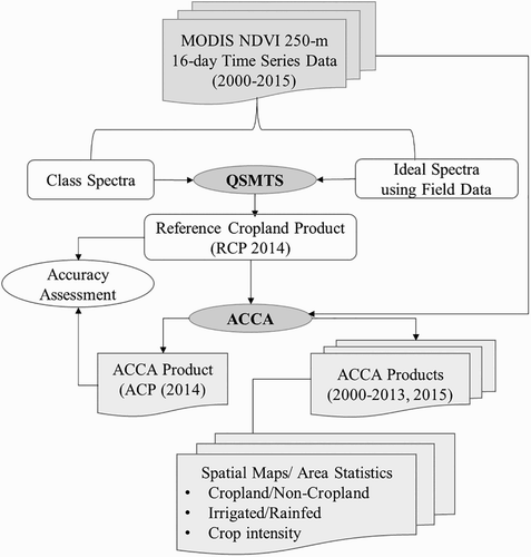
The schematic representation of the data analysis implemented using the QSMTs and the ACCA algorithms are shown in Figure 1. Basically, the analysis approach includes: (1) creating cropland masks based on the best available datasets, (2) developing ideal spectra based on precise ground knowledge and MODIS time-series data, (3) classifying MODIS time-series data using masks to generate class spectra, and (4) performing QSMTs to match class spectra with ideal spectra and determine the RCPs.

Figure 1. Methodology overview. Methodology workflow showing the integrated analysis of MODIS-NDVI time-series data using QSMTs and ACCA.

3.1. Cropland extent and related masks

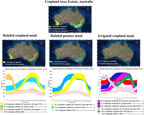
This research began by creating and refining cropland masks. First, we created a baseline nominal 1-km cropland mask (BCM-1 km) based on available coarse resolution data (Teluguntla et al. 2015b). This was followed by refinement of the baseline 1-km mask using MODIS 250-m 16-day time-series data to create refined and much improved baseline 250-m cropland mask (BCM-250 m) (Figure 2). The process is explained in Sections 3.1.1 and 3.1.2.

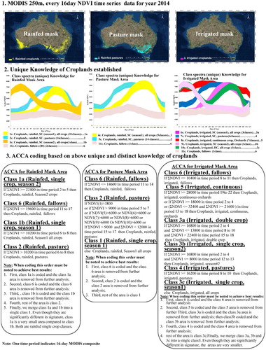
Figure 2. Three cropland masks of Australia and the development of ideal spectral signatures (ISSs) for each of these masks. Development of the three cropland masks is defined in Section 3.1. Using precise ground data and MODIS 250 m time-series data, unique and distinctly separable ISSs of the three masks were a total of 13 classes: (a) 4 for the rainfed mask, (b) 3 for the pasture mask, and (c) 6 for the irrigated-mask. The cropland fallow signature was common across. The total 13 classes can be combined to 6 unique classes by combining similar classes across masks.

3.1.1. Baseline nominal 1-km cropland mask (BCM-1 km) of Australia

Initially, we made use of BCM-1 km developed by Teluguntla et al. (2015b). The BCM-1 km was created by Teluguntla et al. (2015b) by conducting a very thorough spatial analysis of the four best available global cropland studies (Biradar et al. 2009; Friedl et al. 2010, 1; Pittman et al. 2010, 3; Thenkabail et al. 2009b; Thenkabail et al. 2010, 2; Yu et al. 2013, 4.). This resulted in a BCM-1 km (Teluguntla et al. 2015b) for the entire world, from which Australia was extracted. We determined that there was 69.5 million hectares of croplands in Australia as per BCM-1 km.

3.1.2. Baseline nominal 250-m cropland mask (BCM-250 m) of Australia

There are a number of limitations in BCM-1 km. First, it includes significant non-croplands. This is because some of the primary data used have cropland classes that are vague. For example, some of the cropland classes in these four studies have significant non-croplands which is as a result of the definition issues (how croplands are defined) and mixed classes (a class that has a mixture of croplands and other land cover class). Second, coarse resolution nature of BCM-1 km pixels have significant proportion of pixels where cropland proportion is very small (e.g. pixels with < 10% being cropped is also defined a cropland pixel). What this means is that in a single 1-km coarse resolution pixel (each pixel is 100 hectares), only a fraction of a pixel is croplands (i.e. 10 hectares in a 100-hectare pixel area is actually croplands). In such cases, higher resolution pixels can be used to separate croplands from non-croplands.

So, in order to obtain a more refined and accurate cropland mask, we took the BCM-1 km for Australia (Teluguntla et al. 2015b) and used MODIS 250-m 16-day time-series red and near infrared (NIR) band data as well as NDVI data of MODIS to study and sieve out non-croplands and retain only the croplands. We used the year 2014 MODIS 250-m 16-day time-series data stack to classify and plot: (a) red versus NIR bi-spectral plots (Thenkabail, Schull, and Turral 2005), (b) NDVI time-series signatures plots (Thenkabail et al. 2009b), and synthesize with (c) secondary data from the Department of Agriculture and Water Resources (2010) to discern, identify, and eliminate non-cropland pixels within BCE-1 km cropland extent. Extensive sets of submeter to 5-m data from very high spatial resolution imagery (Very High Resolution Imagery, VHRI) such as from Quickbird, IKONOS, and Worldview were used to ensure that cropland areas were clearly differentiated from non-croplands. This led to obtain a baseline cropland mask at 250-m (BCK-250 m) for Australia (Figure 2).

We determined that there was 62.1 million hectares of croplands in Australia as per BCM-250 m (Figure 2) relative to 69.5 million hectares as per BCM-1 km (Teluguntla et al. 2015b), a reduction of massive 7.4 million hectares. Cropland extent mask at 250-m is further divided into (Figure 2): (a) rainfed cropland mask, (b) rainfed pasture mask, and (c) irrigated cropland mask. Irrigated areas were identified based on earlier works of Thenkabail et al. (2009b), and secondary data from the Geoscience Australia and Department of Agriculture and Water Resources (2010). Any expansion of croplands into non-croplands areas in Australia is less than 0.5% of the total cropland area per year (personal discussions with Australian experts during 2014 field visit) and hence it is sufficient to work within the 250-m cropland masks (Figure 2) to understand cropland dynamics, year-after-year. An independent accuracy assessment was performed on the cropland masks to ensure its validity. Accuracies of the BCM-250 m were determined using an independent submeter to 5-m data which provided an overall accuracy (OA) of 98% (Table 5) and the results were compared with another independent cropland map (Salmon et al. 2015) which showed an OA of 96% (Table 8). These results are further discussed in detail later at appropriate portion of the text (Sections 7.1.1 and 7.2.1; Tables 5 and 8).

3.2. Creating RCPs of Australia using QSMTs

The RCPs were developed based on QSMTs which are traditionally developed for hyperspectral data analysis of minerals (Homayouni and Roux 2004). Time-series data, such as the monthly NDVI data from MODIS 250 m, are similar to hyperspectral data; hundreds of months in time-series data replacing tens or hundreds of bands in hyperspectral data (Thenkabail et al. 2007a). QSMTs involve matching time-series MODIS 250 m NDVI of class spectra derived from classification algorithms such as ISOCLASS or k-means clustering (Jensen 2009) with ideal or target spectra of MODIS 250 m NDVI produced based on field-collected reference data and comparing how well the two match in terms of: (a) shape and (b) magnitude.

3.2.1. Creating ideal spectra of croplands using MODIS time-series data and ground data

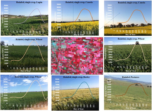
The generation of ideal spectra requires precise knowledge of the croplands which was gathered through extensive field visits (Table 1). These sample locations were overlaid on the MODIS 250 m 16-day composite NDVI data to determine cropland characteristics (Figure 3) allowing us to identify unique signatures for many croplands such as ‘rainfed, single crop, lupin’, ‘rainfed, single crop, wheat’, ‘rainfed, pasture’, etc. Figure 3 illustrates these signatures for several cases of rainfed croplands. Similar signatures were developed for irrigated and pasture as well.

Figure 3. Ideal spectral library of crops. Illustration of few ground data samples collected throughout Australia and their t time-series MODIS 250 m NDVI ideal spectra profiles.

Similar categories or classes were then combined to generate ideal spectra of a group. For example, within the rainfed cropland mask, there were four distinct cropland classes (see Figure 2(a)). These four groups of ideal spectra were: (1) croplands, rainfed, single crop during Season 1, with all crops combined together (n = 722); (2) croplands, rainfed, pasture (n = 89); (3) croplands, rainfed, single crop during Season 2, with all crops combined together (n = 4); and (4) cropland, fallow, rainfed (n = 100). Ground data samples (Table 1) were used to overlay on pasture mask (Figure 2(b)) to generate three distinct ideal spectra of cropland pasture mask (Figure 2(b)): (1) croplands, rainfed, single crop during Season 1, with all crops combined (n = 93); (2) croplands, rainfed, pasture (n = 45); and (3) croplands, fallows (n = 7). Separating croplands from cropland pastures has been demonstrated earlier by others (e. g. Begue et al. 2014; Esch et al. 2014; Müller et al. 2015) in different parts of the world. In Australia, cropland pasture is a major component of cultivated landscapes and it is important to accurately separate it from croplands. Finally, there were six distinctive classes in the irrigated-mask (Figure 2(c)), resulting in the ideal spectra (Figure 2(c)): (1) croplands, irrigated, single crop (Season 1), all crops combined (n = 16); (2) croplands, irrigated, single crop, pasture (n = 19); (3) croplands, irrigated, continuous crops, orchards (n = 6); (4) croplands, irrigated, single crop (Season 2), all crops (n = 8); (5) croplands, irrigated, double crop, all crops (n = 9); and (6) cropland, fallows (n = 21). So, overall there were 13 classes. When generating these spectra, we typically considered about 99% of the pixel signatures with about 1% noise removed.

Overall, from the three cropland masks (rainfed, pasture, and irrigated masks, Figure 2), we established 13 distinct ideal spectra (see Figure 2(a–c)) that can be accurately separated from one another using MODIS 250 m resolution 16-day composite time-series NDVI data and the masks. As shown in Figure 2, the 13 classes can be further combined to 6 unique classes. This is because similar classes from the different masks such as (Figure 2): (a) rainfed cropland class in the rainfed mask is combined with rainfed cropland class from the pasture mask, (b) rainfed pasture class from the rainfed mask is combined with rainfed pasture class of the pasture mask, or (c) cropland fallow classes from the rainfed, irrigated, and pasture masks are distinctly similar. Irrigated double crop was ignored and combined with irrigated single crop since irrigated double crop in Australia, as a proportion of overall irrigated cropland class is negligible. The class variability is shown in the thickness of the ideal spectral curves (Figure 2(c)) and constitutes 99% of all the variability for each class. In Figure 2, we have coded the 13 classes to 6 similar classes across the masks. Overall, having these six distinct classes allowed us to code these broad very useful classes in agriculture and reproduce the same classes accurately year-after-year automatically using the algorithm discussed in next sections.

3.2.2. Class spectra generation through ISOCALSS clustering

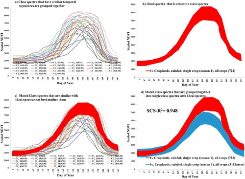
Initially, for each of the masks (Figure 2), 50–100 classes were established through the use of the ISOCLASS clustering algorithm in ERDAS Imagine (Campbell and Wynne. 2011; Jensen 2009). Figure 4(a) illustrates 27 similar classes in terms of their MODIS–NDVI time-series signatures from the rainfed mask. There were 100 initial classes, of which 27 similar ones are plotted in Figure 4(a).

Figure 4. Illustration of SCS R², a QSMT method, to group, match, assess, identify, and label classes. (a) Class spectra: group similar class spectra (e.g. class #’s 3,6,7, 9, … .,41, 44; total 27 similar classes from rainfed mask classification) obtained from ISOCLASS clustering classification, (b) ideal spectra: obtain an ideal spectra from the spectral library that closely matches with the grouped class spectra, (c) class spectra (Figure 4(a)) matched with ideal spectra (Figure 4(b)) using SCS R² values (SCS R² values varied between 0.83 and 0.994, with 26 of 27classes having SCS R-square values of 0.9 or greater), and (d) group of class spectra matched with ideal spectra: combine all similar class spectra into one group and match with ideal spectra which resulted in an SCS R² value of 0.96 leading to labeling of the class spectral classes as similar name as ideal spectral label. So, the class name in this example is: croplands, rainfed, single crop (Season 1), all crops or mixed crops.

3.2.3. Matching class spectra with ideal spectra through spectral correlation similarity R-square values

In this study, we used spectral correlation similarity R-square (SCS R²) values, the most powerful of all the QSMTs in land cover studies (Thenkabail et al. 2007a). SCS R² values are a shape measure that typically produces values between 0 and 1 (theoretically between −1 and +1). Since, negative values have no meaning here, they are ignored. However, it is extremely rare to have negative values at all. The general rule is that the greater the SCS R² values, the greater the similarity between class spectra and target spectra. Figure 4 illustrates how some of these class spectra (Figure 4(a)) were grouped and matched with relevant ideal spectra (e.g. Figure 4(b)).

The process involved: (a) grouping similar classes of class spectra (Figure 4(a)); (b) identifying ideal spectra that were representative of this group of class spectra (Figure 4(b)); (c) overlying ideal spectra on the group of class spectra (Figure 4(c)) and determining their SCS R² values; and (d) matching the average of the grouped class spectra with the ideal spectra (Figure 4(d)) showing both qualitative spectral matching as well as quantitative spectral matching (Figure 4(d)). The QSMTs SCS R² values are shown within brackets of the class legend in Figure 4(c). Classes in each group have an SCS R² value of 0.90 or higher (one case is 0.83). When all similar class spectra are grouped and matched with the ideal spectra an R² value of 0.96 was achieved (Figure 4(d)).

The same process was repeated for all the hundreds of classes from all three (rainfed, pasture, and irrigated) masks (Section 3.2.2). These hundreds of classes were then grouped into six broad, distinct, highly separable, similar groups of classes, and matched with ideal spectra (Section 3.2.1) which resulted in an SCS R² values of 0.89–0.99 (Table 2) between the class spectra and the ideal spectra.

Table 2. SCS R² values, a QSMT, matching class spectra with ideal spectra.

		Class spectra
Ideal spectra		1c	2c	3c	4c	5c	6c
	1i	0.948
	2i		0.977
	3i			0.993
	4i				0.993
	5i					0.883
	6i						0.99

Note: (a) 1i, 2i, 3i, 4i, 5i, and 6i represent ideal spectra developed from ground data and

(b) 1c, 2c, 3c, 4c, 5c, and 6c represent class spectra obtained from unsupervised classification.

3.3. Final label of classes for the RCP for the year 2014 (RCP2014)

After preliminary labeling of classes as defined in the previous section, the process of final labeling of the RCP2014 involved the following additional steps: (A) using extensive ground reference data (Table 1) to further verify class names; (B) use of VHRI (submeter to 5 m) such as Worldview, Quickbird, and IKONOS; and (C) use of secondary data from other published work (e.g. Australia’s National Systems DLCD by Lymburner et al. 2014; Thenkabail et al. 2012; Teluguntla et al. 2015b).

Ground reference data (Table 1) provided information on croplands versus non-croplands, irrigation versus rainfed, and crop type. There were 4111 ground reference data samples of which we had 1458 samples available for training algorithm, class identification, and labeling classes. Section 2.1 provides more information of the type of information consistently available for all ground samples. Information about croplands and non-croplands were visually extracted from VHRI. Occasionally, information pertaining to irrigated versus rainfed watering methods were also extracted (e.g. center pivots and irrigation channels). Secondary data were available in form of maps and published literature for selected subregions of Australia (e.g. Salmon et al. 2015; Australian National Systems DLCD by Lymburner et al. 2014; Thenkabail et al. 2012; Teluguntla et al. 2015b). These secondary data sources either helped further affirm what was already identified and\or helped in labeling classes when no other data were available for a class. Cropping intensity was derived by combining field observations with MODIS time-series NDVI signatures that showed whether there was a single crop, double crop, or continuous crop (e.g. plantations) present for the calendar year. Finally, numerous initial classes (e.g. Figure 4(a), Section 3.2.2) were merged into highly distinguishable pure classes (e.g. Table 2, Section 3.2.3) where the final class labels were established through detailed investigation supported by ground and secondary data (Section 3.3). The accuracies of these classes are evaluated using two independent sample datasets (Table 1): (a) 1488 internal validation samples and (b) 1465 samples from an independent accuracy assessment team which the mapping team does not have access.

4. ACCA overview

The goal of rule-based ACCA (Figure 5) is to enable production of cropland products year-after-year, automatically, and accurately without having to go through tedious, rigorous, time, and resource consuming methods and approaches involved in producing RCPs (Section 3.2). The ACCA algorithm (Figure 5) developed in this project involved the following steps. First, was the production of an accurate RCP2014 (Section 3.0 and its subsections). Second, was to develop ACCA algorithm rules (Section 4.1), which was done in ERDAS Imagine modeler, in order to accurately replicate RCP2014 classes in ACCA-derived classes for the year 2014 (ACP2014) using MODIS 250 m NDVI 16-day composite data for the year 2014. Third, was to apply ACCA algorithm for independent years (2000–2013 and 2015) using MODIS 250 m NDVI 16-day composite data (2000–2013 and 2015) to produce accurately ACCA-derived cropland products for those years (ACP2000–ACP2013 and ACP2015). Since MODIS Terra/Aqua data is available from the year 2000 to foreseeable future along with data continuity plans through the Visible Infrared Imaging Radiometer Suite (VIIRS) onboard the National Polar-orbiting Operational Environmental Satellite System (NPOESS), developing ACCA for MODIS will allow cropland products generation for the past (hind-cast; ACCA developed for 2014 and was successfully applied for the years 2000–2013), present (now-cast for the year 2014 for which ACCA was developed), and future years (future-cast; ACCA was successfully applied for 2015 and similarly can be applied for any future year).

Figure 5. An automated cropland classification algorithm (ACCA) for Australia that can be used to compute six cropland classes as well as croplands versus non-croplands year-after-year automatically and accurately.

4.1. Development of ACCA rules for re-producing cropland products

The ACCA algorithm was developed based on the accurate knowledge captured in the RCP2014 (Figure 5). The process of developing ACCA from RCP2014 has three broad steps (Figure 5): (1) taking MODIS 250 m, NDVI time-series for the year 2014 for rainfed, pasture, and irrigated-masks (Figure 5, Step 1); (2) capturing the unique knowledge of each class (e.g. NDVI time-series of the classes) of each mask (Figure 5, Step 2); and (3) writing the ACCA codes that capture the knowledge established in Step2. For example, within the rainfed cropland mask, we coded (Figure 5, Step 3): If ∑NDVI > = 22,400 in time periods 2–5 (of the 23 yearly, 16-day MODIS–NDVI time-series composites) then the class is: croplands, rainfed, Season 2. Similarly, within the irrigated cropland mask areas, we coded (Figure 5, Step 3): If ∑NDVI < = 10,400 in time periods 8–11, then the class is: croplands, irrigated, fallows. The process of such ACCA coding is completed for all classes (Figure 5, Step 3) in ERDAS Imagine modeler. The ACCA algorithm (Figure 5, Step 3) is then applied on the year 2014 and the resulting product (ACP2014) is then compared with RCP2014. The process is repeated, by tweaking ACCA codes, to ensure maximum separability of the classes resulting in perfect or near perfect match between ACP2014 classes with RCP2014 classes. The ACCA algorithm was modified until the accuracies of the six classes of ACP2014 reached an accuracy of 85% or higher when compared with the six classes of RCP2014 in a pixel by pixel error matrix comparison.

4.1.1. ACCA algorithm automation

Once a robust ACCA algorithm (Figure 5) was developed based on MODIS 250-m 16-day time-series data, it was coded in ERDAS Imagine modeler (.gmd file). In order to automatically run and produce cropland products (e.g. Figure 7) for independent years, MODIS 250 m, 16-day NDVI time-series data of Australia for independent years needs to be compiled. ACCA algorithm was applied for the independent years, 2000 through 2013, and the year 2015 to rapidly produce (ACP2000–ACP2013, and ACP2015) as illustrated for selected years in Figure 7 and Figure 9. Apart from applying ACCA algorithm codes on any given year (past, present, or future) using MODIS 250-m 16-day time-series data, no other interaction, analysis, or interpretation is required.

5. Area calculations

Area of cropland is an important metric. Area is computed taking two important factors:

1. Subpixel composition of pixels, so actual areas or subpixel areas (SPAs) are established and

2. Seasonality of pixels, so areas are computed based on intensity (e.g. single, double, triple, and continuous cropping).

The MODIS 250-m full pixel areas (FPAs) is ∼6.25 hectares per pixel. However, at times, only a portion of the ∼6.25 hectares pixel area is in croplands with the rest of the pixel left fallow. We, therefore, model the SPAs which reflect actual areas. Computation of actual areas or SPAs requires us to multiply FPAs with cropland area fractions (CAFs) (Thenkabail et al. 2007b):Once the final class maps are obtained, the image is re-projected to GDA_1994_Australia_Albers and FPAs are established for each class. There is a rigorous methodology for establishing CAFs (see Thenkabail et al. 2007b).

Then the class phenology is then determined to understand whether a class is single crop, double crop, triple crop, or continuous crop in a calendar year. When a pixel is single cropped, the area is computed once; when pixel is double cropped, the area is computed twice; and when the pixel has continuous cropping (e.g. plantations), the area is computed once.

Net cropland areas refer to actual cropland area whether the cropland is planted or left fallow. It does not account for cropping intensity. However, it does include permanent crops (e.g. plantations). Gross cropland areas (GCAs) are sum of the planted areas during different seasons (e.g. single, double, and triple cropping in a year). GCAs also include permanent crops. Detailed methods of area calculations are provided in Thenkabail et al. (2007b) and Velpuri et al. (2009).

6. Accuracy assessment

Comprehensive accuracy assessments for the RCPs and the ACPs were performed using standard error matrices (Congalton 1991, 2009, 2015; Congalton et al. 2014; Olofsson et al. 2014; Stehman et al. 2012; Tilman et al. 2011; Tsendbazar, De Bruin, and Herold 2015; Tsendbazar et al. 2016).

First, the accuracies of the RCP for the baseline year 2014 (RCP2014) were established using two sets of ground data collected during 2014 and withheld from ACCA model development (Table 1):

1. First set of 1488 independent validation samples and

2. Second set of 1465 validation samples collected by an external team, blinded to the team performing the analysis.

Second, the ACP accuracies for the year 2014 (ACP2014) were performed using RCP2014 based on an error/similarity matrix involving all pixels of two products.

Third, accuracies of the independent years, 2000–2013 and 2015, were determined Through a pixel by pixel error matrix of ACCA-derived cropland product for the year 2005 (ACP2005) with the 2005 product of Salmon et al. (2015);

1. With an independent Australian National system map, also produced using MODIS data for the years 2000–2008;

2. Comparison with published NASA climate data to compare cropland versus cropland fallows for the years 2000 through 2014; and

3. Comparison with Australia National statistics versus ACCA-derived cropland statistics for the years 2000–2013.

Thus, a robust and detailed accuracy assessment was performed both for the RCPs and ACPs.

7. Results

First, we will present and discuss the results of the reference cropland data products for the baseline year of 2014 (RCP2014, Section 7.1) for Australia developed using QSMTs involving SCS R² method. Second, we will discuss accuracies of RCP2014 (Section 7.1.1) established using ground data also for the baseline year 2014. Third, the discussion will focus on the ability of ACCA algorithm to replicate croplands for the baseline year 2014 (ACP2014, Section 7.2), followed by accuracies of these products. Fourth, ACCA algorithms ability to automatically and accurately compute cropland products for the independent years (ACP2000–2013 and ACP2015, Section 7.3) will be established. Finally, cropland statistics and areas were compared with the statistics of other sources like Australian National system and other International sources (e.g. Food and Agricultural Organization (FAO), Section 8.0).

7.1. RCP2014 for Australia

Overall, RCP2014 of Australia has six distinct cropland classes (Figure 6) as mapped using the QSMTs and MODIS 250 m time-series data for the baseline year 2014. Actual cropland areas (or SPAs) of the six classes were estimated as 58.55 Mha with pasture and 30.80 Mha without pasture for the year 2014 (Table 3). The areas were calculated separately for Season 1 (June–October), Season 2 (November–March), and continuous (e.g. plantations) (Table 3). The annualized areas are also reported in Table 3. Of the total 58.55 Mha, Class 1 (croplands, rainfed, single crop, mixed, or all crops) with 45.5%, and Class 2 (croplands, rainfed, single crop, pastures) with 46% dominate Australian croplands (Table 3). When only croplands are considered, it is clear that in Australia Class 1 (croplands, rainfed, single crop, mixed, or all crops) is overwhelming with 86.6% of the total cropland areas (30.80 Mha). In contrast, irrigated areas (Class 3 and Class 5) add up to just 5.1%. The rest, 8.3%, was cropland fallows (Table 3).

Figure 6. RCP of the year 2014 (RCP2014) for Australia at 250 m.

Note: 1. Total area of cropland (with pasture): 58.55 Mha, total area of cropland (without pasture): 30.80 Mha; 2. the % within brackets in the legend classes are as % of 58.55 Mha.

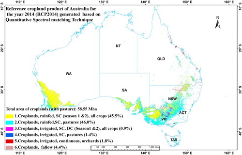
Table 3. Cropland areas of Australia for the year 2014 showing the net cropland areas (without considering cropland intensity) and annualized cropland areas (considering cropland intensity).

	Net Area Season1 (NAS1)			Net Area Season2 (NAS2)			Net Area Continuous (NAC)			Annualized Area (AA) = NAS1 + NAS2 + NAC
	FPA^a	CAF^b	SPA^c	FPA^a	CAF^b	SPA^c	FPA^a	CAF^b	SPA^c	Season 1 + Season 2 +  Continous	Percent of total cropland + pasture area	Percent of total cropland area
Class name	Mha	%	Mha	Mha	%	Mha	Mha	%	Mha	Mha	%	%
1. Croplands, rainfed, SC (Seasons 1 and 2), all crops	28.12	93.2	26.21	0.472	97.6	0.46	N/A	N/A	N/A	26.67	45.5	86.6
2. Croplands, rainfed, SC, pastures	28.34	95.0	26.91	N/A	N/A	N/A	N/A	N/A	N/A	26.91	46.0
3. Croplands, irrigated, SC, DC (Seasons 1 and 2), all crops	0.46	90.3	0.42	0.106	98.6	0.10	N/A	N/A	N/A	0.52	0.9	1.7
4. Croplands, irrigated, SC, pastures	0.85	99.0	0.84	N/A	N/A	N/A	N/A	N/A	N/A	0.84	1.4
5. Croplands, irrigated, continuous, orchards	N/A	N/A	N/A	N/A	N/A	N/A	1.12	94.8	1.06	1.06	1.8	3.4
6. Croplands, fallow^d	2.55	100	2.55							2.55	4.4	8.3
							Total 1: 1–6 (Mha)			58.55	100.00
							Total 2: 1, 3, 5, 6 (Mha)			30.80		100.00

Note: The areas also show cropland with and without pasture. SC = single crop: DC = double crop.

^aFPA (Full pixel area) is determined by reprojecting geographic projection to GDA 1994 Albers projection for Australia.

^bCAF (Crop area fraction) is determined by developing relationship between average NDVI of growing season with percent cover based on literature.

^cSPA(Sub pixel area) = FPA × CAF.

^dCAF for fallow fraction area (FFA) = 100.

7.1.1. Accuracy of RCP2014

The accuracy of the RCP for the baseline year 2014 (RCP2014) was tested using two sets of validation data. The first validation data had a total of 1488 ground data samples. These were overlaid on the final cropland map (Figure 6) and an error matrix (Table 4) was derived. The OA of the six class map was 83.1% with kappa coefficient = 0.75 (Table 4). The user’s and producer’s accuracies of each of the unique crop classes were also high. For example, cropland Class 1 (croplands, rainfed, single crop, mixed, or all crops) which occupies 86.6% of all cropland areas showed a producer’s accuracy of 83.4% indicating that 83.4% of Class 1 pixels (in ground reference data) were correctly classified as rainfed cropland pixels. As a user, 92.1% of the pixels classified as Class 1 by QSMT were indeed Class 1 (Table 4). All other classes except cropland pasture have very good producer’s and user’s accuracies. In comparison, cropland pastures have significant commission and omission errors. This is mainly due to the fact variability in pasture is very high since they are cultivated and harvested at varying times and at any given time they are in varying growth stages. Also, natural grasses and sometimes crops like rainfed barley gets confused with pasture. We suggest that future studies put greater emphasis in gathering significantly higher proportion of cropland pasture ground data to better train algorithms.

Table 4. Accuracy error matrix of the RCP of Australia for the year 2014 (RCP2014 on Y-axis) based on validation ground dataset #1 obtained during field visit (X-axis) also conducted during the year 2014.

		Ground reference data
		1. Croplands, rainfed, all crops	2. Croplands, rainfed, pastures	3. Croplands, irrigated, all crops	4. Croplands, irrigated, Pastures	5. Croplands, irrigated, continuous, orchards	6. Croplands, fallow	7. Non-croplands	Row total (SMT Classified)	Commission error^s
RCP2014	1. Croplands, rainfed, all crops	700	42	0	0	1	0	17	760	5.7%
	2. Croplands, rainfed, pastures	133	101	0	0	5	0	18	257	53.7%
	3. Croplands, irrigated, all crops	0	0	54	2	0	0	0	56	3.6%
	4. Croplands, irrigated, pastures	0	0	9	60	0	0	0	69	13.0%
	5. Croplands, irrigated, continuous, Orchards	0	0	1	1	58	0	7	67	3.0%
	6. Croplands, fallow	2	1	0	0	0	140	0	143	2.1%
	7. Non-croplands	4	8	0	0	0	1	123	136	9.6%
	Column total (ground reference data)	839	152	64	63	64	141	165	1488
	Omission error^b	16.6%	33.6%	15.6%	4.8%	9.4%	0.7%	25.5%
	Producer accuracy^c	83.4%	66.4%	84.4%	95.2%	90.6%	99.3%	74.5%
	User accuracy^d	92.1%	39.3%	96.4%	87.0%	86.6%	97.9%	90.4%
	Over all accuracy^e									83.1%
									Kappa^f	0.747

^aCommission error : pixels that belong to another class but labeled as this class.

^bOmission error: pixels that belong to this class, but are labeled to another class.

^cProducer accuracy: as a producer, 83.4% of the cropland pixels of class 1 in ground reference data were correctly classified as cropland pixels of class 1 in RCP2014.

^dUser accuracy: as a user, 92.1% of the pixels classified as croplands pixels of class 1by RCP2014 were indeed croplands.

^eOverall accuracy = total classification accuracy.

^fKappa value compares observed accuracy (overall) with expected accuracy (random chance).

A second set of validation ground data samples of 1465 samples were available with the independent team and blinded from the team developing the product. Their accuracy assessment showed an overall accuracy of 98.2% with kappa coefficient of 0.91 for croplands versus non-croplands (Table 5). A special feature of this accuracy was that they used balanced (proportionate samples for crop and non-crop) in their accuracy assessment.

Table 5. Accuracy Error matrix for the RCP for the year 2014 (RCP2014) conducted by external independent evaluation team based on validation dataset #2 obtained during field visit of year 2014.

	Ground reference data
		1. Cropland	2. Non-cropland	Row total	Commission error^a
RCP 2014	1.Cropland	102	13	115	11.3%
	2. Non-cropland	4	810	814	0.5%
	Column total	106	823	929
	Omission error^b	3.8%	1.6%
	Producer accuracy^c	96.2%	98.4%
	User accuracy^d	88.7%	99.5%
	Overall accuracy^e				98.2%
				Kappa^f	0.91

^aCommission error : pixels that belong to another class but labeled as this class.

^bOmission error : pixels that belong to this class, but are labelled to another class.

^cProducer accuracy: 96.2% of the cropland pixels of class 1 in ground reference data were correctly classified as cropland pixels of Class 1 in RCP2014.

^dUser accuracy: 88.7% of the pixels classified as croplands pixels of class 1by RCP2014 were indeed croplands.

^eOverall accuracy = total classification accuracy.

^fkappa value compares observed accuracy (overall) with expected accuracy (random chance).

These accuracies clearly demonstrated the high level of confidence one can have with the reference RCP2014 product.

7.2. ACCA2014 for Australia

Based on the ACCA algorithm developed using the knowledge base from the RCP2014 product, the ACCA-derived cropland product for the year 2014 (ACP2014) is produced (Figure 7). The goal of the ACCA was to derive ACP that closely and accurately replicates the RCP (Figure 6). So, the ACP2014 (Figure 7) has same classes as the RCP2014 (Figure 6).

Figure 7. ACCA algorithm derived cropland product for the year 2014 (ACP2014) for Australia at 250 m.

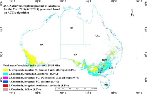
A class by class comparison of the RCP2014 with ACP2014 is provided in Table 6. Overall, 13,650,958 pixels were mapped as cropland pixels for Australia. The comparative results in Table 6 (with spatial view in Figure 6 versus Figure 7) clearly demonstrate that ACCA algorithm produced product (ACP2014) was able to replicate the RCP2014 with a great degree of accuracy. For example, 99.4% of the pixels mapped as Class 1 (cropland, rainfed, single crop, mixed, or all crops) in RCP2014 were also mapped as Class 1 in ACP2014. A comparison of the percentage of pixels in each of the six classes from RCP2014 and ACP2014 also showed great degree of similarity (Table 6), clearly indicating the performance capability of the ACCA algorithm.

Table 6. Comparison of the statistics from RCP2014 with ACP2014.

Class description	RCP 2014^a	Percent of croplands	ACP 2014^b	Percent of croplands	Percent of ACP2014^b to RCP2014^a
Name	#Pixels	%	#Pixels	%	%
1. Croplands, rainfed, all crops	620,5071	45.5	6,170,793	45.2	99.4
2. Croplands, rainfed, pastures	6,363,457	46.6	6,400,516	46.9	100.6
3. Croplands, irrigated, all crops	105,109	0.8	95,748	0.7	91.1
4. Croplands, irrigated, pastures	189,325	1.4	191,920	1.4	101.4
5. Croplands, irrigated, continuous	237,235	1.7	243,680	1.8	102.7
6. Croplands, fallow	550,761	4.0	548,301	4.0	99.6
Total croplands	13,650,958	100.0	13,650,958	100.0

Note: The statistics of the reference cropland products of the year 2014 (RCP2014) were compared with the statistics of the ACCA-derived cropland product of the year 2014 (ACP2014).

^aReference cropland product for the year 2014 (RCP2014) was produced using QSMTs.

^bAutomated cropland classification algorithm (ACCA) derived cropland product for the year 2014 (ACP 2014) is produced using ACCA algorithm.

7.2.1. Accuracies/ similarities of ACP2014 when compared with the RCP2014

A pixel by pixel comparison between the ACP2014 (Figure 7) with RCP2014 (Figure 6) is provided in Table 7. The results show ACP2014 was replicating the RCP2014 with an overall accuracy/similarity of 89.4% (kappa = 0.814). The producer’s and user’s accuracies were also very high. As a producer, 89.7% of Class 1 pixels (in RCP) were correctly classified as rainfed cropland pixels by the ACCA product ACP (Table 7). As a user, 90.2% of the pixels classified as Class 1 by ACCA were indeed Class 1 (Table 7). These results show the ACCA algorithm can automatically and accurately classify croplands that match the reference product. We compared the ACP2014 map with two other national products. First, the results of ACP2014 for croplands versus non-cropland were compared with the 500-m Global Rainfed and Irrigated Paddy Croplands (GRIPC500 m) data produced by Salmon et al. (Table 8) with high degree of overall accuracies (96.3%), kappa coefficient (0.76) and also very good producer’s and user’s accuracies (Table 8). However, given that GRIPC500 is a MODIS 500-m product compared to ACP2014 which is a MODIS 250-m product, there is bound to be commission and omission errors as a result of pixel resolution differences. Furthermore, some differences also rise from definitions used in mapping. Second, the Australian state-wise irrigated cropland areas produced by ACP2014 were compared with the irrigated area estimates provided by the United Nations Food and Agricultural Organization (FAO) (Figure 8). The results indicated an excellent match between the two studies (Figure 8) with an R² value of 0.97.

Figure 8. ACP2014 versus FAO state by state statistics for irrigated cropland areas of Australia.

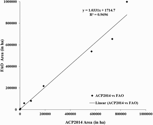
Table 7. ACP2014 versus RCP2014 error/similarity matrix.

		RCP2014
		1. Croplands, rainfed, all crops	2. Croplands, rainfed, pastures	3. Croplands, irrigated, all crops	4. Croplands, irrigated, pastures	5. Croplands, irrigated, continuous	6. Croplands, fallow	Row total SMT classified	Commission error^a
ACP2014	1. Croplands, rainfed, all crops	556,5497	621,112	0	0	0	18,462	6,205,071	10.3%
	2. Croplands, rainfed, pastures	520,562	575,3513	0	0	0	89,382	6,363,457	9.6%
	3. Croplands, irrigated, all crops	0	0	75,551	14647	9723	5188	105,109	28.1%
	4. Croplands, irrigated, pastures	0	0	8927	157,372	23,026	0	189,325	16.9%
	5. Croplands, irrigated, continuous, Orchards	0	0	6901	19,849	210,242	243	237,235	11.4%
	6. Croplands, fallow	84,734	25891	4369	52	689	435,026	550,761	21.0%
	Column total (ACCA classified)	6,170,793	6,400,516	95,748	191,920	243,680	548,301	13,650,958
	Omission error^b	9.8%	10.1%	21.1%	18.0%	13.7%	20.7%
	Producer accuracy^c	89.7%	90.4%	71.9%	83.1%	88.6%	79.0%
	User accuracy^d	90.2%	89.9%	78.9%	82.0%	86.3%	79.3%
	Overall accuracy^e								89.4%
								Kappa^f	0.814

Note: Error/similarity matrix comparing ACCA generated cropland product for the year 2014 (ACP2014) with reference cropland product for the year 2014 (RCP2014).

^aCommission error:pixels that belong to another class but labeled as this class.

^bOmission error pixels that belong to this class, but are labelled to another class.

^cProducer accuracy:89.7% of the cropland pixels of class 1 in RCP2014 (reference product) were correctly classified as cropland pixels of Class 1 in ACP2014 (ACCA-derived product).

^dUser accuracy: 90.2% of the pixels classified as croplands pixels of class 1 (by ACCA algorithm) were indeed croplands.

^eOverall accuracy = total classification accuracy.

^fKappa value compares observed accuracy (overall) with expected accuracy (random chance).

Table 8. ACP2014 versus GRIPC500 m (Salmon et al. 2015) accuracy assessment.

	GRIPC^g
		1. Cropland	2. Non-cropland	Row total	Commission error^a
ACP 2014	1. Cropland	10051903	3665084	13716987	26.7%
	2. Non-cropland	2157017	141845510	144002527	1.5%
	Column total	12208920	145510594	157719514
	Omission error^b	17.7%	2.5%
	Producer accuracy^c	82.3%	97.5%
	User accuracy^d	73.3%	98.5%
	Overall accuracy^e				96.3%
				Kappa^f	0.755

Note: Accuracy of ACCA generated cropland product for the year 2014 (ACP2014) versus GRIPC500 m (Salmon et al. 2015).

^aCommission error: pixels that belong to another class but labeled as this class.

^bOmission error: pixels that belong to this class, but are labeled to another class.

^cProducer accuracy: as a producer, 82.3% of the cropland pixels in GRIPC were correctly classified as cropland pixels in ACP2014 (ACCA algorithm derived product).

^dUser accuracy: as a user, 73.3% of the pixels classified as croplands pixels (by ACCA algorithm) were indeed croplands.

^eOverall accuracy = total classification accuracy.

^fKappa value compares observed accuracy (overall) with expected accuracy (random chance).

^gGRIPC = global rainfed and irrigated cropland map at 500 m resolution produced by Salmon et al. (2015).

7.2.2. Irrigated areas of Australia

Irrigated areas calculated in this study were compared with several other studies such as FAO AQUASTAT (2011); Australian National Statistics, GRIPC (Salmon et al. 2015); and DLCD (Lymburner et al. 2014) (Table 9). This study reported a total irrigated area (TIA) of 2.38 Mha for Season 1 which was comparable to the (Table 9): (a) actual irrigated area for Season 1 as per FAO AQUASTAT which was 2.56 Mha and (b) actual irrigated areas reported by the Australian National Statistics which was 2.54 Mha. The DLCD reports irrigated as 897,966 hectares, which is way below any other estimates. Whereas, GRIPC (Salmon et al. 2015) reported equipped irrigated areas (EIA) of 8.8 Mha based on 500 m MODIS imagery, which is way above any other estimates. In contrast, FAO AQUASTAT reports EIA as 4.07 Mha. Even though GRIPC areas are FPAs, they are still far higher than what is reported by FAO AQUASTAT. Salmon et al. (2015) reported in their GRIPC500 m paper that their study overestimated irrigated areas as a result of many reasons that include (Salmon et al. 2015): (a) mapping some of the dryland rainfed wheat areas as irrigated, (b) not accounting for dramatic changes in irrigation pattern of Australia during 2004–2006, and (c) not accounting for policy changes such as the Australian National Water Initiative that was adopted in 2004 wherein environmental flows of Murray–Darling river system were restored significantly reducing irrigated areas. As a result of these issues there are going to be significant differences in estimates of irrigated areas. However, such factors were accounted in this research as well as in FAO AQUASTAT, resulting in a good match between the two studies. Thereby, the actual irrigated area of Australia was estimated at around 2.46 Mha as of year 2014. In Season 2, this study reported TIA of 0.10 Mha. Other studies do not report the second season irrigated areas.

Table 9. Comparison of Australia’s irrigated areas from different studies.

State	Area equipped for irrigation^a (ha)	Area actually irrigated FAO AQUASTAT^b (ha)	Australia National Statistics (ANS)^c (ha)	GCEV2^d This Study (ha)	GRIPC^e (ha)	DLCD^f (ha)
Australian Capital Territory	253	253		51	333	57
New South Wales	1,534,678	998,753	994,000	849,377	3,676,518	130,933
Northern Territory	30,462	7250	7000	2970	16,466	3008
Queensland	1,101,836	539,257	539,000	568,760	605,300	450,660
South Australia	306,616	217,941	217,000	187,532	1,083,047	23,451
Tasmania	135,051	80,642	81,000	87,529	182,894	80,174
Victoria	873,819	654,543	648,000	733,623	2,756,052	209,067
Western Australia	86,250	59,482	60,000	33,056	456,444	617
Australia total	4,068,965	2,558,121	2,546,000	2,462,899	8,777,052	897,966

Note: Comparison of irrigated areas for each state of Australia between this study and several other sources.

^aArea equipped for irrigation (AEI) was obtained from FAO AQUASTAT. Depending on water availability and other factors certain proportion of AEI gets cultivated each year.

^bFAO AQUASTAT = UN Food and Agricultural Organization (FAO) reported irrigated areas (http://www.fao.org/nr/water/aquastat/main/index.stm).

^cAustralian Bureau of Statistics (2008), irrigated areas for year 2005–2006, ca# 4618.0, http://www.abs.gov.au/AUSSTATS.

^dGCEV2 = Australia cropland extent produced at 250 m using MODIS data for the year 2014.

^eGRIPC = global rainfed and irrigated croplands produced using 500 m MODIS data for the Year 2005 by Salmon et al. (2015).

^fDLCD = dynamic land cover dataset (DLCD) reported irrigated areas produced by Geoscience Australia based on irrigated areas over a decade.

7.3. ACCA-derived cropland data product of Australia for the years 2000 through 2013 (ACP2000–ACP2013) and for the year 2015 (ACP2015)

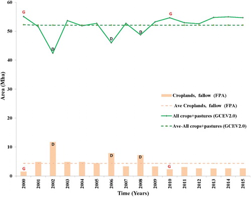
Once the ACCA algorithm (Figure 5) was tested and verified (Section 7.2), it was applied to 15 independent years (2000–2013 and 2015). The only requirement to apply the ACCA to any year (past, present, or future) is that the data type and scaling used in the original algorithm remain the same. In this case, MODIS 16-day composite 250-m NDVI time-series data were compiled for each of the 15 independent years and the ACCA algorithm was applied to each of the years without any further user interaction. The output, consistently produced the same six classes each year, for years 2000–2013 and 2015 (e.g. Figure 9 illustrating 4 years). In Figure 10, we illustrate these for six years (two droughts, two normal, and two good years). From these outputs, we calculated cropland areas (Classes 1–5) and cropland fallow areas (Class 6) from the year 2000 to 2015 and plotted them in Figure 11. The three worst drought years in Australia’s 100 years’ historical record were the years 2002, 2006, and 2008 (Murray-Darling Authority 2009; Australian Bureau of Meteorology 2009; and NASA Earth Observatory, n.d.). This illustration clearly implies climate sensitivity of ACCA algorithm in determining croplands versus cropland fallows.

Figure 9. ACCA-derived cropland products for the past years (hind-cast) and future years (future-cast) for Australia. ACCA algorithm that was developed based on extensive ground data for the years 2014 was applied for the past years (2000–2013) and for a future year (2015). We have illustrated here ACCA-derived cropland products for 4 years: three past years (ACCA-derived cropland product for the year 2002 or ACP2002, ACP2004, and ACP2010) and for a future year (ACP2015). ACCA algorithm can be applied to develop similar products for the any future year.

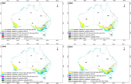
Figure 10. ACCA algorithm derived croplands (ACPs) for drought and non-drought years for Australia. Croplands versus cropland fallows computed using ACCA algorithm are shown for two: (a) worst drought years: 2002 and 2006 (ACP2000 and ACP2006), (b) normal years: 2003 and 2004 (ACP2003 and ACP2004), and (c) good years: 2000 and 2010 (ACP2000 and ACP2010).

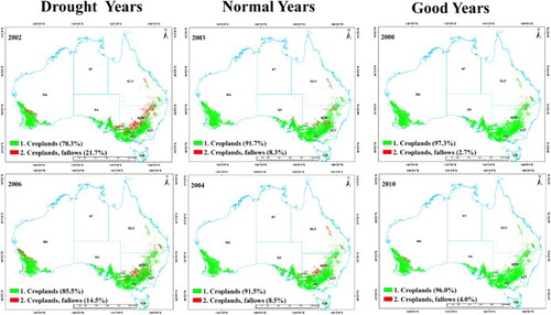
Figure 11. ACP2000 to ACP2015 derived cropland areas versus cropland fallow areas.

Note: the dotted lines indicate mean of 16 years.

8. Discussions

The spatial, temporal, and spectral specifications of MODIS are considered as highly suitable for land use and land cover (LULC) classifications, especially for cropland extent and area mapping (Hentze, Thonfeld, and Menz 2016). Others (Dong et al. 2015; Gumma et al. 2016; Zhang et al. 2015; Zhou et al. 2016) showed the ability of phenology-based algorithms in paddy rice mapping by using MODIS time-series and/or by integrating MODIS with other higher spatial resolution data such as Landsat 8 OLI images. This research further re-iterates the strength of MODIS time-series data in cropland and/or specific LULC mapping.

Agricultural croplands are often mapped year-after-year or season-after-season by extensive and rigorous cropland mapping methods and approaches (e.g. Becker-Reshef et al. 2010; Ozdogan and Gutman 2008; Pervez, Budde, and Rowland 2014; Pittman et al. 2010; Thenkabail et al. 2007a, 2009a; Waldner, Canto, and Defourny 2015; Wardlow, Egbert, and Kastens 2007; Yu et al. 2013). We used some of these methods (Section 3.0 and its subsections) to produce an accurate RCP with six classes for the year 2014 (RCP2014, Figure 6). We then developed ACCA algorithm (Section 4.0 and its subsections) using the precise knowledge ingrained in the RCP2014 (Figure 6). ACCA algorithm was then used to accurately reproduce RCP2014, resulting in ACCA-derived cropland product for the year 2014 (ACP2014). ACCA algorithm, developed based on the year 2014 MODIS 16-day time-series data, was then used to consistently hind-cast and future-cast the same six classes as illustrated for four distinct years (Figure 9):

1. Three past years: 2002 (ACP2002) – a drought year, 2004 (ACP2004) – a normal year, and 2010 (ACP2010) – a wet year, and

2. One future year: 2015 (ACP2015).

When MODIS 16-day time-series data becomes available for the entire year 2016 and beyond, we can produce cropland products for those years just as we produced for one future-year (2015) for which the entire year data were available when we wrote this paper. In this process, all we need is the MODIS 16-day time-series data for any given year and for any given area (Australia in this case) that is similar to MODIS 16-day time-series data used to produce RCP2014 of Australia. Once the MODIS 16-day time-series data stacks are available for the past or the future years, ACCA algorithm is run using the same process used to produce six class ACP2014 (Figure 7 and Section 4.0 and its subsections) resulting in similar six class cropland products for other years (e.g. Figure 9 showing three past-years: 2002, 2004, and 2010, and one future-year: 2015, relative to year 2014). Statistics derived for all the 16 years: (i) hind-cast years (2000–2013), (ii) current year 2014 – the year for which the ACCA algorithm was developed, and (iii) future-cast year (2015) is plotted for croplands versus cropland fallows and shown in Figure 11 and their spatial distribution illustrated for few years (Figure 10). Thereby, the ability of ACCA algorithm to clearly capture cropland product year-after-year: past, present, and future (e.g. Figures 9–11) is clearly demonstrated in this research.

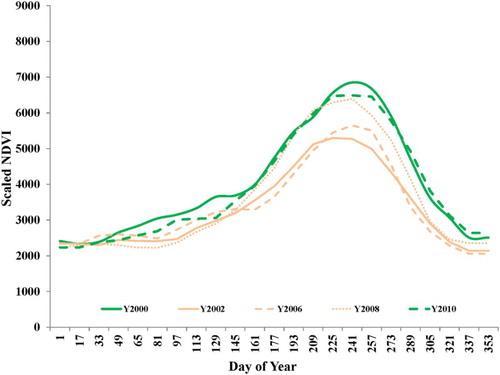
The reliability of the cropland product were evaluated using 100-years climate data (Murray-Darling Basin Authority 2009, Bureau of Meteorology, Australian Government: http://www.bom.gov.au/climate/current/month/aus/summary.shtml) which clearly established that three of the worst 100-year drought years were 2002, 2006, and 2008, whereas two of the best climate years were 2000 and 2010. ACCA algorithm precisely captured these events (Figure 11) by highlighting the three worst drought years (2002, 2006, and 2008) by showing during these years, highest cropland fallows and lowest cropland areas (Figure 11, with some spatial illustrations in Figure 10). Furthermore, drought years also had lowest crop vigor (Figure 12) on existing croplands of those years.

Figure 12. Cropland vigor during worst drought years versus the best above normal years. Mean MODIS 250 m NDVIs of Australia’s croplands during the: (a) three worst drought years of the century (2002, 2006, and 2008) versus (b) two very good years (2000 and 2010).

Furthermore, this research has shown the strength of ACCA algorithm developed based on knowledge capture and coding in accurate cropland mapping over very large areas such as continents. The main advantages of the ACCA algorithm are its: (a) development which is based on precise knowledge obtained from extensive field visits, (b) ability to automatically, and accurately compute croplands year-after-year, and (c) simplicity in concept and application. As long as knowledge is clearly deciphered as outlined in Figure 5 and Section 4.0, it can be encoded precisely to achieve accurate results.

In addition to the lowest cropland areas, these years show the highest fallow croplands in the ACP2002, ACP2006, and ACP2008 products (see marked ‘D’ for drought in Figure 11). In contrast, the two best years (highest precipitation years), 2000 and 2010 (Murray-Darling Authority 2009; Australian Bureau of Meteorology 2009; NASA Earth Observatory, n.d.) also showed highest cropland areas as well as lowest cropland fallow areas (see marked ‘G’ for good in Figure 11). These results further validate our ACCA algorithm’s ability to accurately, automatically, and rapidly provide cropland products, including croplands versus cropland fallows, as well as derive their cropland areas (e.g. Figures 10 and 11). Figure 12 also reveals that the three worst drought years (2002, 2006, and 2008) of the century had significantly lower MODIS 250 m NDVIs for the croplands of Australia relative to good years (2000 and 2010). For example, during the worst drought year of 2002, cropland fallows were as high as ∼12 Mha relative to just 2 Mha during the best year (2000), a difference of nearly 10 Mha (Figure 11). Furthermore, the mean MODIS 250 m scaled-NDVI during peak growing period was only about 5200 during the worst drought year of 2002 when compared with a scaled-NDVI of about 6800 during the peak growing period of the best year (2000) (Figure 12). This demonstrates that not only do the cropland fallow areas increase significantly and cropland areas decrease significantly during drought years (Figure 11), the areas that are cropped also have significantly lower in biomass and biomass vigor (Figure 12). The combination of these two factors will have a significant impact on the quantum of food produced – both in terms of quantity and quality. This is because, when the cropland extent reduces significantly, production also reduces significantly. In drought years, vigor is lesser even when a crop exists. Such croplands with less vigor results not only in quantity reduction but also quality reduction. Hence the study clearly demonstrates the ACCA algorithm ability to picture the food security scenarios, year-after-year and clearly demonstrates that the ACCA algorithm is sensitive to climate variability. This approach and method is expected to work better in large industrial agriculture such as Australia, USA, Europe, and Canada. But how well such methods work in subsistence agriculture such as in Africa, India, and China where often the field sizes are small needs to be tested. Approach may require us to use MODIS time-series along with Landsat and/or Sentinel time-series. Such an approach will allow not only rich temporal resolutions but also rich spatial resolutions. Furthermore, major crops such as wheat, rice, and corn are grown extensively over large contiguous areas, field after field, even when filed sizes are small in India and China. In Africa, challenges will be much higher. But, with rich ground data along with a combination of MODIS and Landsat and/or Sentinel time-series data should help address these issues.

Others have used machine learning algorithms like the ensembles of decision trees in random forest algorithms (Gislason, Benediktsson, and Sveinsson 2006; Hentze, Thonfeld, and Menz 2016; Tatsumi et al. 2015), and spectral angle mapper (Kumar et al. 2016) for cropland mapping. They are fast and simple to train, and predictive but a major limitation is to have sufficient number of training samples in each class to be mapped to get an accurate outcome. For example, if we are mapping irrigated versus rainfed, we will need training data in entire range of irrigated and entire range of rainfed to ensure we capture accurate outcome in classification. Other machine learning algorithms like the support vector machines (Mountrakis, Im, and Ogole 2011) can be very inefficient and complex to train. The ACCA algorithm is simple to train and implement using a set of recursive rules that captures the accurate knowledge base in the RCPs and codifies it. ACCA algorithm is then validated for the year(s) or season(s) it is developed, as well as independent years to ensure its robustness. Once this is achieved, ACCA algorithm is applied to hind-cast, now-cast, and future-cast and produce cropland products automatically and accurately as we have demonstrated in this study.

Our attempt to develop crop type maps for Australia at MODIS 250 m resolution was not successful. This was because almost all rainfed crops, which occupy about 95% of Australia’s croplands, have the same phenology, are grown during the same rainy season, and often have two or more crops in a MODIS 250 m (6.25 hectare) nominal pixel resolution. These factors resulted in the MODIS 250-m NDVI time-series ideal spectra for crop types too similar to one another, with only a minor difference in magnitude throughout the growing season. Hence it was not feasible to separate them without large omission and commission errors. Crop types are separated in some other studies (e.g. Kumar et al. 2016; Kontgis, Schneider, and Ozdogan 2015; Mariotto et al. 2013; Marshall and Thenkabail 2015; Qin et al. 2015). However, these studies used, one or more of the following: (a) high spatial resolution (e.g. 30 m) data, (b) high spatial resolution with high temporal resolution (e.g. several 30 m images during the season), and (c) very large and homogeneous field size (e.g. US Midwest for simple cases such as corn versus soybeans).

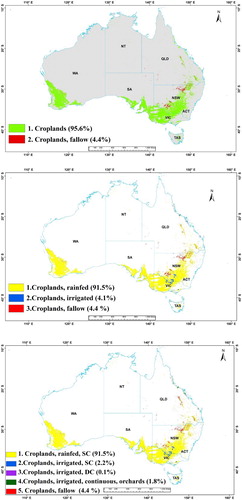
We use ACCA algorithm to produce other key cropland products: (1) cropland extent, (2) irrigated versus rainfed, (3) cropping intensity, and (4) croplands versus cropland fallows. These products are ideal for assessing food security scenarios. For example, of the 58.55 Mha (Table 3) of total croplands (croplands and cropland pasture) in Australia during the year 2014, 95.6% was croplands (91.5% rainfed and 4.1% irrigated) and 4.4% was cropland fallows (Figure 13, top image). Year 2014 was a normal year in terms of rainfall (478 mm). Given that the overwhelming proportion of the Australia’s croplands are rainfed, normal rainfall is very critical to agriculture. The Product 2 (Figure 13, middle image) shows the spatial distribution of the rainfed cropland (91.5%) as opposed to irrigated croplands (4.1%), with rest 4.4% being cropland fallows during 2014. Australia has very low percentage of irrigated croplands; these are located overwhelmingly in Murray–Darling river basins on the east. Finally, as per Product 3 (Figure 13, bottom image), rainfed single crops (92.1%) dominate, followed by irrigated single crop (2%), irrigated continuous crop consisting of orchards and plantations (1.7%), and negligible irrigated double crop (0.1%). There is tremendous value in each of these products in helping to answer questions related to cropland water use (e.g. single crop in a season will have much less water used compared to double crop), food security (e.g. area cropped versus area left fallows), and green water use (rainfed croplands) and blue water use (irrigated croplands).

Figure 13. Cropland products of Australia. (a) Product 1: croplands versus non-croplands; (b) Product 2: irrigated versus rainfed; and (c) Product 3: cropping intensity: croplands with single, double, or triple cropping as well as cropland fallows.

Uncertainty in croplands products is very low for most classes as seen in accuracy assessment error matrices (Tables 4, 5 and 7). Highest uncertainty exists for cropland pasture class. Greater reliability of this class and further improvement in uncertainties in other classes can be achieved by series of measures that include: (a) gathering greater number of samples, (b) better spatial distribution of sample locations, (c) better understanding of the variability in the cropland pasture class, (d) collecting data over multiple years and seasons, (e) incorporating ancillary data (e.g. climate) in addition to remote sensing in data cubes, and (f) a whole host of other parameters such as integrating multi-sensor data (e.g. MODIS with Landsat, and Sentinel).

Finally, the value of these maps and products are many. First, the same six cropland classes (e.g. Figure 7 and 9) can be generated for entire Australia year-after-year rapidly, routinely, automatically, and accurately using ACCA algorithm and MODIS 250-m 16-day time-series data. Second, we can hind-cast, now-cast, and future-cast the same six cropland classes year-after-year automatically using ACCA algorithm using MODIS 250-m 16-day time-series data. Third, cropland area statistics, at national and subnational level, can be computed from these. Fourth, the ACCA algorithm can help determine spatial distribution and areas of croplands versus cropland fallows during any year that can help highlight and quantify extent and magnitude of drought, normal, and good years. Fifth, all of these products can be used in assessing food and water security analysis. Nevertheless, there is significant scope for further improvement in these products. For example, high resolution remote sensing data (e.g. Landsat 30-m or Sentinel-2 10-m or 20-m) can be used to produce even better nominal baseline cropland masks at 30-m (BCM-30 m) than the baseline cropland mask at 250-m (BCM-250 m). More recently, Australian Collaborative Land Use and Management Program (ACLUMP), Bureau of Rural Sciences, has produced a 50-m product (http://www.agriculture.gov.au/abares/aclump/Pages/land-use/data-download.aspx) at four times during the study period. Nevertheless, routine, repetitive, and rapid computation of croplands versus non-croplands for the years past, present, and future (e.g. Figure 11 and 10) is only possible through 16-day time-series data available from MODIS. Furthermore, MODIS offers consistent data for the entire world, routinely acquired twice a day and time-composited for 16-day periods, offering clean near cloud free data of the entire world. Such high quality near cloud free data time-series at higher resolution like 50-m or 30-m for the entire world is still quite some time away even with combination of Landsat and Sentinel. Further MODIS 16-day data offers other advantages such as the study of cropping intensity (Figures 12 and 13) or irrigated and rainfed (e.g. Figure 13). Also, computing challenges of handling 50 and 30-m data still exist and are significant. However, with recent advances in cloud computing and machine learning algorithms, the future of remote sensing in cropland studies should plan to integrate 50 or 30-m high resolution data from satellite systems such as Landsat and Sentinels with temporal capabilities of MODIS 250-m data.

9. Conclusions

This research developed and demonstrated a novel ACCA to (a) hind-cast, (b) now-cast, and (c) future-cast cropland products (croplands versus cropland fallows, cropland extent/areas, cropping intensity, irrigation versus rainfed) year-after-year using MODIS 250-m NDVI 16-day time-series data. First, an RCP was generated for the year 2014 (RCP2014) using extensive ground data, MODIS 250 m NDVI 16-day time-series data, and QSMTs. The RCP2014 accuracies achieved: (a) an OA of 83.1% with kappa coefficient of 0.75 for six cropland classes involving rainfed, irrigated, and pasture classes and (b) an OA of 98.2% with kappa coefficient of 0.91 for croplands versus non-croplands. Second, a rule-based ACCA algorithm was developed based on the knowledge captured by the RCP2014. The ACCA developed cropland product for the year 2014 (ACP2014) was then validated with RCP2014. Based on a pixel-by-pixel comparison (13,650,958 cropland pixels) of the two products, the error/similarity matrix produced an overall accuracy/similarity of 89.4% (kappa = 0.814) with six class: (a) producer’s accuracies varying between 72% and 90% and (b) user’s accuracies varying between 79% and 90%. Third, ACPs for individual years 2000–2013 and 2015 (ACP2000–ACP2014 and ACP2015) were computed automatically and rapidly using ACCA algorithm applied on MODIS–NDVI time-series for these years. Hind-casting was performed for 14 years (years 2000 through 2013) by successfully and accurately applying ACCA algorithm developed for the year 2014 data on time-series MODIS data of the past years (2001–2013). Future-casting was performed for one year (year 2015) by successfully and accurately applying ACCA algorithm developed for the year 2014 on time-series MODIS data of a future year (2015). The cropland areas versus cropland fallow areas of the 16 years (2000 through 2015) showed that the three worst drought years (2002, 2006, and 2008) of the century for Australia were clearly captured by ACP2002, ACP2006, and ACP2008 – these drought years had highest cropland fallow areas. Fourth, ACCA algorithm successfully captured year by year variations on cropland versus cropland fallow areas as well as variations in year by year cropland vigor. These two factors (change in cropland extent\areas and change in cropland vigor) help determine crop productivity variations resulting in food security assessments and policy formulations. Fifth, the cropland products were released through https://croplands.org/app/map and sample data and algorithms are released through http://geography.wr.usgs.gov/science/croplands/algorithms/australia_250m.html

Acknowledgements

The authors gratefully acknowledge the project funding provided by the National Aeronautics and Space Administration (NASA) grant number: NNH13AV82I through its MEaSUREs (Making Earth System Data Records for Use in Research Environments) initiative. The United States Geological Survey (USGS) provided supplemental funding from other direct and indirect means through its Land Change Science (LCS), and Land Remote Sensing (LRS) programs as well as its Climate and Land Use Change Mission Area. Finally, authors would like to thank Prof. Alfredo Huete and Dr Rakhesh Devadas, University of Technology Sydney, Sydney for the comprehensive field work support and coordination in Australia.

Disclosure statement

No potential conflict of interest was reported by the author(s).

ORCID

Pardhasaradhi Teluguntla http://orcid.org/0000-0001-8060-9841

Prasad S. Thenkabail http://orcid.org/0000-0002-2182-8822

Jun Xiong http://orcid.org/0000-0002-2320-0780

Murali Krishna Gumma http://orcid.org/0000-0002-3760-3935

Russell G. Congalton http://orcid.org/0000-0003-3891-2163

Adam Oliphant http://orcid.org/0000-0001-8622-7932

Justin Poehnelt http://orcid.org/0000-0001-5914-4269

Kamini Yadav http://orcid.org/0000-0002-7560-8884

Mahesh Rao http://orcid.org/0000-0002-8689-5209

Richard Massey http://orcid.org/0000-0002-4831-8718

Additional information

Funding

This work was supported by NASA MEaSUREs (grant number NNH13AV82I); U.S. Geological Survey provided supplemental funding from other direct and indirect means through its Land Change Science (LCS), and Land Remote Sensing (LRS) programs as well as its Climate and Land Use Change Mission Area.

References

- ABARES (Australian Bureau of Agricultural and Resource Economics and Sciences). 2011. “Agricultural Commodities: December Quarter 2011; 2011b, Agricultural Commodity Statistics 2011; 2011c, Global Food Security: Facts, Issues and Implications.” Science and Economic Insights 1. http://www.abs.gov.au/ausstats/[email protected]/Lookup/by%20Subject/1301.0∼2012∼Main%20Features∼Farming%20in%20Australia∼207.
- de Abelleyra, D., and S. R. Verón. 2014. “Comparison of Different BRDF Correction Methods to Generate Daily Normalized MODIS 250 m Time-Series.” Remote Sensing of Environment 140: 46–59. doi: 10.1016/j.rse.2013.08.019
- Australia National Farmers Federation. 2012. “Farm facts”. Last Accessed February 8 2016. http://www.nff.org.au/farm-facts.html.
- Australian Bureau of Meteorology. 2009. “ Climate Education: Drought”. Accessed December 10 2015. http://www.bom.gov.au/.
- Australian Bureau of Statistics. 2008. “ Water use on Australian Farms”, 2005-06 ca# 4618.0 http://www.abs.gov.au/AUSSTATS.
- Becker-Reshef, I., C. Justice, M. Sullivan, E. Vermote, C. Tucker, A. Anyamba, J. Small, E. Pak, E. Masuoka, and J. Schmaltz. 2010. “Monitoring Global Croplands with Coarse Resolution Earth Observations: The Global Agriculture Monitoring GLAM Project.” Remote Sensing 2: 1589–1609. doi: 10.3390/rs2061589
- Begue, A., E. Vintrou, A. Saad, and P. Hiernaux. 2014. “Differences Between Cropland and Rangeland MODIS Phenology Start-Of-Season in Mali.” International Journal of Applied Earth Observation and Geoinformation 31: 167–170. doi: 10.1016/j.jag.2014.03.024
- Biggs, T., P. Thenkabail, M. Gumma, C. Scott, G. Parthasaradhi, and H. Turral. 2006. “Irrigated Area Mapping in Heterogeneous Landscapes with MODIS Time-Series, Ground Truth and Census Data, Krishna Basin, India.” International Journal of Remote Sensing 27: 4245–4266. doi: 10.1080/01431160600851801
- Biradar, C. M., P. S. Thenkabail, P. Noojipady, Y. Li, V. Dheeravath, H. Turral, M. Velpuri, M. K. Gumma, O. R. P. Gangalakunta, and X. L. Cai. 2009. “A Global map of Rainfed Cropland Areas GMRCA at the end of Last Millennium Using Remote Sensing.” International Journal of Applied Earth Observation and Geoinformation 11: 114–129. doi: 10.1016/j.jag.2008.11.002
- Campbell, J. B., and R. H. Wynne. 2011. Introduction to Remote Sensing. New York: Guilford Press.
- Chen, J., J. Chen, A. Liao, X. Cao, L. Chen, X. Chen, C. He, G. Han, S. Peng, and M. Lu. 2015. “Global Land Cover Mapping at 30 m Resolution: A POK-Based Operational Approach.” ISPRS Journal of Photogrammetry and Remote Sensing 103: 7–27. doi: 10.1016/j.isprsjprs.2014.09.002
- Cohen, W. B., and S. N. Goward. 2004. “Landsat’s Role in Ecological Applications of Remote Sensing.” Bioscience 54: 535–545. doi: 10.1641/0006-3568(2004)054[0535:LRIEAO]2.0.CO;2
- Congalton, R. 1991. “A Review of Assessing the Accuracy of Classifications of Remotely Sensed Data.” Remote Sensing of Environmen. 37: 35–46. doi: 10.1016/0034-4257(91)90048-B
- Congalton, R. G. 2009. “19 Accuracy and Error Analysis of Global and Local Maps: Lessons Learned and Future Considerations.” In Remote Sensing of Global Croplands for Food Security, edited by P. S. Thenkabail, C. M. Biradar, H. Turral, and J. G. Lyon, 441–458. Boca Raton, FL: CRC Press. doi: 10.1201/9781420090109.sec7
- Congalton, R. G. 2015. “Assessing Positional and Thematic Accuracies of Maps Generated From Remotely Sensed Data.” In “Remote Sensing Handbook” Three Volume set: Remotely Sensed Data Characterization, Classification, and Accuracies, edited by P. S. Thenkabail, 583–602. Boca Raton, FL: Taylor and Francis/CRC Press 800+.
- Congalton, R. G., J. Gu, K. Yadav, P. Thenkabail, and M. Ozdogan. 2014. “Global Land Cover Mapping: A Review and Uncertainty Analysis.” Remote Sensing 6: 12070–12093. doi: 10.3390/rs61212070
- Crist, Eric P., and Richard C. Cicone. 1984. “A Physically-based Transformation of Thematic Mapper Data---The TM Tasseled Cap.” IEEE Transactions on Geoscience and Remote Sensing 3: 256–263. doi: 10.1109/TGRS.1984.350619
- De Fries, R. S., and J. C. W. Chan. 2000. “Multiple Criteria for Evaluating Machine Learning Algorithms for Land Cover Classification From Satellite Data.” Remote Sensing of Environment, 743: 503–515. doi: 10.1016/S0034-4257(00)00142-5
- De Fries, R., M. Hansen, J. Townshend, and R. Sohlberg. 1998. “Global Land Cover Classifications at 8 km Spatial Resolution: the use of Training Data Derived From Landsat Imagery in Decision Tree Classifiers.” International Journal of Remote Sensing 19: 3141–3168. doi: 10.1080/014311698214235
- Department of Agriculture and Water Resources, Govt of Australia. 2010. Accessed July 10 2016. http://data.daff.gov.au/anrdl/metadata_files/pa_luav4g9abl07811a00.xml.
- Dheeravath, V., P. Thenkabail, G. Chandrakantha, P. Noojipady, G. Reddy, C. Biradar, M. K. Gumma, and M. Velpuri. 2010. “Irrigated Areas of India Derived Using MODIS 500 m Time-Series for the Years 2001–2003.” ISPRS Journal of Photogrammetry and Remote Sensing 65: 42–59. doi: 10.1016/j.isprsjprs.2009.08.004
- Dong, J., X. Xiao, W. Kou, Y. Qin, G. Zhang, L. Li, C. Jin, Y. Zhou, J. Wang, and C. Biradar. 2015. “Tracking the Dynamics of Paddy Rice Planting Area in 1986–2010 Through Time-Series Landsat Images and Phenology-Based Algorithms.” Remote Sensing of Environment 160: 99–113. doi: 10.1016/j.rse.2015.01.004
- Duro, D. C., S. E. Franklin, and M. G. Dubé. 2012. “A Comparison of Pixel-Based and Object-Based Image Analysis with Selected Machine Learning Algorithms for the Classification of Agricultural Landscapes Using SPOT-5 HRG Imagery.” Remote Sensing of Environment 118: 259–272. doi: 10.1016/j.rse.2011.11.020
- Duveiller, G., R. Lopez-Lozano, and A. Cescatti. 2015. “Exploiting the Multi-Angularity of the MODIS Temporal Signal to Identify Spatially Homogeneous Vegetation Cover: A Demonstration for Agricultural Monitoring Applications.” Remote Sensing of Environment 166: 61–77. doi: 10.1016/j.rse.2015.06.001
- Egorov, A. V., M. C. Hansen, D. P. Roy, A. Kommareddy, and P. V. Potapov. 2015. “Image Interpretation-Guided Supervised Classification Using Nested Segmentation.” Remote Sensing of Environment 165: 135–147. doi: 10.1016/j.rse.2015.04.022
- Esch, T., A. Metz, M. Marconcini, and M. Keil. 2014. “Combined use of Multi-Seasonal High and Medium Resolution Satellite Imagery for Parcel-Related Mapping of Cropland and Grassland.” International Journal of Applied Earth Observation and Geoinformation 28: 230–237. doi: 10.1016/j.jag.2013.12.007
- FAO. 2011. AQUASTAT “Global Map of irrigation Areas.” Accessed November 22 2016. http://www.fao.org/nr/water/aquastat/irrigationmap/AUS/index.stm.
- Foley, J. A., R. DeFries, G. P. Asner, C. Barford, G. Bonan, S. R. Carpenter, F. S. Chapin, M. T. Coe, G. C. Daily, and H. K. Gibbs. 2005. “Global Consequences of Land use.” science 309: 570–574. doi: 10.1126/science.1111772
- Foley, J. A., N. Ramankutty, K. A. Brauman, E. S. Cassidy, J. S. Gerber, M. Johnston, N. D. Mueller, C. O’Connell, D. K. Ray, and P. C. West. 2011. “Solutions for a Cultivated Planet.” Nature 478: 337–342. doi: 10.1038/nature10452
- Friedl, M. A., and C. E. Brodley. 1997. “Decision Tree Classification of Land Cover From Remotely Sensed Data.” Remote Sensing of Environment 61: 399–409. doi: 10.1016/S0034-4257(97)00049-7
- Friedl, M. A., D. Sulla-Menashe, B. Tan, A. Schneider, N. Ramankutty, A. Sibley, and X. Huang. 2010. “MODIS Collection 5 Global Land Cover: Algorithm Refinements and Characterization of new Datasets.” Remote Sensing of Environment 114: 168–182. doi: 10.1016/j.rse.2009.08.016
- Funk, C. C., and M. E. Brown. 2009. “Declining Global per Capita Agricultural Production and Warming Oceans Threaten Food Security.” Food Security 1: 271–289. doi: 10.1007/s12571-009-0026-y
- Gislason, P. O., J. A. Benediktsson, and J. R. Sveinsson. 2006. “Random Forests for Land Cover Classification.” Pattern Recognition Letters 27: 294–300. doi: 10.1016/j.patrec.2005.08.011
- Gumma, M.K., A. Nelson, P.S. Thenkabail, and A.N. Singh. 2011. “Mapping Rice Areas of South Asia Using MODIS Multitemporal Data.” Journal of Applied Remote Sensing 5: 053547–053547–053526.
- Gumma, M. K., P. S. Thenkabail, A. Maunahan, S. Islam, and A. Nelson. 2014. “Mapping Seasonal Rice Cropland Extent and Area in the High Cropping Intensity Environment of Bangladesh Using MODIS 500 m Data for the Year 2010.” ISPRS Journal of Photogrammetry and Remote Sensing 91: 98–113. doi: 10.1016/j.isprsjprs.2014.02.007
- Gumma, M. K., P. S. Thenkabail, P. Teluguntla, M. N. Rao, I. A. Mohammed, and A. M. Whitbread. 2016. “Mapping Rice-Fallow Cropland Areas for Short-Season Grain Legumes Intensification in South Asia Using MODIS 250 m Time-Series Data.” International Journal of Digital Earth 9 (10): 1–23. doi: 10.1080/17538947.2016.1168489
- Gutman, G., R. Byrnes, I. Masek, S. Covington, C. Justice, S. Franks, and R. Headley. 2008. “Towards Monitoring Land Cover and Land-Use Changes at a Global Scale: The Global Land Survey.” Photogrammetric Engineering and Remote Sensing 74: 6–10.
- Hentze, K., F. Thonfeld, and G. Menz. 2016. “Evaluating Crop Area Mapping From MODIS Time-Series as an Assessment Tool for Zimbabwe’s “Fast Track Land Reform Programme.” PLoS ONE 116: e0156630. doi:10.1371/journal.pone.0156630.
- Homayouni, S., and M. Roux. 2004. “Hyperspectral image analysis for material mapping using spectral matching.” ISPRS Congress Proceedings. http://www.cartesia.org/geodoc/isprs2004/comm7/papers/10.pdf
- Jensen, J.R. 2009. Remote Sensing of the Environment: An Earth Resource Perspective 2/e. Delhi: Pearson Education India.
- Klein Goldewijk, K., A. Beusen, G. Van Drecht, and M. De Vos. 2011. “The HYDE 3.1 Spatially Explicit Database of Human-Induced Global Land-use Change Over the Past 12,000 Years.” Global Ecology and Biogeography 20: 73–86. doi: 10.1111/j.1466-8238.2010.00587.x
- Kontgis, C., A. Schneider, and M. Ozdogan. 2015. “Mapping Rice Paddy Extent and Intensification in the Vietnamese Mekong River Delta with Dense Time Stacks of Landsat Data.” Remote Sensing of Environment 169: 255–269. doi: 10.1016/j.rse.2015.08.004
- Kumar, P., R. Prasad, A. Choudhary, V. N. Mishra, D. K. Gupta, and P. Srivastava. 2016. “A Statistical Significance of Differences in Classification Accuracy of Crop Types Using Different Classification Algorithms.” Geocarto International 1–19. doi:10.1080/10106049.2015.1132483.
- Lary, D. J., A. H. Alavi, A. H. Gandomi, and A. L. Walker. 2016. “Machine Learning in Geosciences and Remote Sensing.” Geoscience Frontiers 71: 3–10. doi: 10.1016/j.gsf.2015.07.003
- Loveland, T., B. Reed, J. Brown, D. Ohlen, Z. Zhu, L. Yang, and J. Merchant. 2000. “Development of a Global Land Cover Characteristics Database and IGBP DISCover From 1 km AVHRR Data.” International Journal of Remote Sensing 21: 1303–1330. doi: 10.1080/014311600210191
- Lymburner, L., P. Tan, N. Mueller, R. Thackway, A. Lewis, M. Thankappan, L. Randall, A. Islam, and U. Senarath. 2014. “ The National Dynamic Land Cover Dataset DLCD”. Record 2011/31.
- Mariotto, I., P. S. Thenkabail, A. Huete, E. T. Slonecker, and A. Platonov. 2013. “Hyperspectral Versus Multispectral Crop-Productivity Modeling and Type Discrimination for the HyspIRI Mission.” Remote Sensing of Environment 139: 291–305. doi: 10.1016/j.rse.2013.08.002
- Marshall, M., and P. Thenkabail. 2015. “Advantage of Hyperspectral EO-1 Hyperion Over Multispectral IKONOS, GeoEye-1, WorldView-2, Landsat ETM+, and MODIS Vegetation Indices in Crop Biomass Estimation.” ISPRS Journal of Photogrammetry and Remote Sensing 108: 205–218. doi: 10.1016/j.isprsjprs.2015.08.001
- Masek, J. G., C. Huang, R. Wolfe, W. Cohen, F. Hall, J. Kutler, and P. Nelson. 2008. “North American Forest Disturbance Mapped From a Decadal Landsat Record.” Remote Sensing of Environment 112: 2914–2926. doi: 10.1016/j.rse.2008.02.010
- Monfreda, C., N. Ramankutty, and J. A. Foley. 2008. “Farming the Planet: 2. Geographic Distribution of Crop Areas, Yields, Physiological Types, and net Primary Production in the Year 2000.” Global Biogeochemical Cycles 22 (1). doi:10.1029/2007GB002947.
- Mountrakis, G., J. Im, and C. Ogole. 2011. “Support Vector Machines in Remote Sensing: A Review.” ISPRS Journal of Photogrammetry and Remote Sensing 66: 247–259. doi: 10.1016/j.isprsjprs.2010.11.001
- Müller, H., P. Rufin, P. Griffiths, A. J. B. Siqueira, and P. Hostert. 2015. “Mining Dense Landsat Time-Series for Separating Cropland and Pasture in a Heterogeneous Brazilian Savanna Landscape.” Remote Sensing of Environment 156: 490–499. doi: 10.1016/j.rse.2014.10.014
- Murray-Darling Basin Authority. 2009. “ River Murray System Drought Update, Issue 21.” Murray-Darling Basin Authority Website. http://www.mdba.gov.au/.
- NASA Earth Observatory n.d. Drought cycles in Australia. Accessed November 22 2016. http://earthobservatory.nasa.gov/Features/WorldOfChange/australia_ndvi.php.
- Olofsson, P., G. M. Foody, M. Herold, S. V. Stehman, C. E. Woodcock, and M. A. Wulder. 2014. “Good Practices for Estimating Area and Assessing Accuracy of Land Change.” Remote Sensing of Environment 148: 42–57. doi: 10.1016/j.rse.2014.02.015
- Ozdogan, M., and G. Gutman. 2008. “A new Methodology to map Irrigated Areas Using Multi-Temporal MODIS and Ancillary Data: An Application Example in the Continental US.” Remote Sensing of Environment 112: 3520–3537. doi: 10.1016/j.rse.2008.04.010
- Ozdogan, M., and C. E. Woodcock. 2006. “Resolution Dependent Errors in Remote Sensing of Cultivated Areas.” Remote Sensing of Environment,103: 203–217. doi: 10.1016/j.rse.2006.04.004
- Pan, Z., Huang, J., Zhou, Q., Wang, L., Cheng, Y., Zhang, H., Blackburn, G.A., J. Yan, and J. Liu. 2015. ‘Mapping Crop Phenology Using NDVI Time-Series Derived From HJ-1 A/B Data.’ International Journal of Applied Earth Observation and Geoinformation 34: 188–197. doi: 10.1016/j.jag.2014.08.011
- Pantazi, X. E., D. Moshou, T. Alexandridis, R. L. Whetton, and A. M. Mouazen. 2016. “Wheat Yield Prediction Using Machine Learning and Advanced Sensing Techniques.” Computers and Electronics in Agriculture 121: 57–65. doi: 10.1016/j.compag.2015.11.018
- Pervez, M. S., M. Budde, and J. Rowland. 2014. “Mapping Irrigated Areas in Afghanistan Over the Past Decade Using MODIS NDVI.” Remote Sensing of Environment 149: 155–165. doi: 10.1016/j.rse.2014.04.008
- Pittman, K., M. C. Hansen, I. Becker-Reshef, P. V. Potapov, and C. O. Justice. 2010. “Estimating Global Cropland Extent with Multi-Year MODIS Data.” Remote Sensing 2: 1844–1863. doi: 10.3390/rs2071844
- Portmann, F. T., S. Siebert, and P. Döll. 2010. “MIRCA2000—Global Monthly Irrigated and Rainfed Crop Areas Around the Year 2000: A new High-Resolution Data set for Agricultural and Hydrological Modeling.” Global Biogeochemical Cycles 24 (1). doi:10.1029/2008GB003435.
- Qin, Y., X. Xiao, J. Dong, Y. Zhou, Z. Zhu, G. Zhang, G. Du, C. Jin, W. Kou, and J. Wang. 2015. “Mapping Paddy Rice Planting Area in Cold Temperate Climate Region Through Analysis of Time-Series Landsat 8 OLI, Landsat 7 ETM+ and MODIS Imagery.” ISPRS Journal of Photogrammetry and Remote Sensing 105: 220–233. doi: 10.1016/j.isprsjprs.2015.04.008
- Ramankutty, N., A.T. Evan, C. Monfreda, and J. A. Foley. 2008. “Farming the Planet: 1. Geographic Distribution of Global Agricultural Lands in the Year 2000.” Global Biogeochemical Cycles, 22 (1). doi:10.1029/2007GB002952.
- Salmon, J. M., M. A. Friedl, S. Frolking, D. Wisser, and E. M. Douglas. 2015. “Global Rain-fed, Irrigated, and Paddy Croplands: A new High Resolution map Derived From Remote Sensing, Crop Inventories and Climate Data.” International Journal of Applied Earth Observation and Geoinformation 38: 321–334. doi: 10.1016/j.jag.2015.01.014
- Shao, Y., and R. S. Lunetta. 2012. “Comparison of Support Vector Machine, Neural Network, and CART Algorithms for the Land-Cover Classification Using Limited Training Data Points.” ISPRS Journal of Photogrammetry and Remote Sensing 70: 78–87. doi: 10.1016/j.isprsjprs.2012.04.001
- Siebert, S., and P. Döll. 2010. “Quantifying Blue and Green Virtual Water Contents in Global Crop Production as Well as Potential Production Losses Without Irrigation.” Journal of Hydrology 384: 198–217. doi: 10.1016/j.jhydrol.2009.07.031
- Siebert, S., F. T. Portmann, and P. Döll. 2010. “Global Patterns of Cropland use Intensity.” Remote Sensing 2: 1625–1643. doi: 10.3390/rs2071625
- Solano, R., K. Didan, A. Jacobson, and A. Huete. 2010. “ MODIS Vegetation Index User’s Guide MOD13 Series.” Vegetation Index and Phenology Lab. Accessed January 24 2016 http://vip.arizona.edu/documents/MODIS/MODIS_VI_UsersGuide_01_2012.pdf.
- Stehman, S. V., P. Olofsson, C. E. Woodcock, M. Herold, and M. A. Friedl. 2012. “A Global Land-Cover Validation Data set, II: Augmenting a Stratified Sampling Design to Estimate Accuracy by Region and Land-Cover Class.” International Journal of Remote Sensing 33: 6975–6993. doi: 10.1080/01431161.2012.695092
- Tatsumi, K., Y. Yamashiki, M. A. C. Torres, and C. L. R. Taipe. 2015. “Crop Classification of Upland Fields Using Random Forest of Time-Series Landsat 7 ETM+ Data.” Computers and Electronics in Agriculture 115: 171–179. doi: 10.1016/j.compag.2015.05.001
- Teluguntla, P., D. Ryu, B. George, J. P. Walker, and H. M. Malano. 2015a. “Mapping Flooded Rice Paddies Using Time-Series of MODIS Imagery in the Krishna River Basin, India.” Remote Sensing 7: 8858–8882.
- Teluguntla, P., P. S. Thenkabail, J. Xiong, M. K. Gumma, C. Giri, C. Milesi, M. Ozdogan, R. Congalton, J. Tilton, T. R. Sankey, R. Massey, A. Phalke, and K. Yadav. 2015b. Global Food Security Support Analysis Data at Nominal 1 km GFSAD1 km Derived From Remote Sensing in Support of Food Security in the Twenty-First Century: Current Achievements and Future Possibilities. Chapter 6, “Remote Sensing Handbook” Volume II: Land Resources: Monitoring, Modeling, and Mapping, 131–159. Boca Raton, FL: Taylor and Francis/CRC Press.
- Thenkabail, P. S. 2015. “Remote Sensing of Land Resources: Monitoring, Modeling, and Mapping Advances Over the Last 50 Years and a Vision for the Future,” Chapter 26. “Remote Sensing Handbook” Volume II: Land Resources Monitoring, Modeling, and Mapping with Remote Sensing, 791–832. Boca Raton, FL: Taylor and Francis/CRC Press, . ISBN 9781482217957 – CAT# K22130..
- Thenkabail, P. S., C. M. Biradar, P. Noojipady, X. Cai, V. Dheeravath, Y. Li, M. Velpuri, M. Gumma, and S. Pandey. 2007b. “Sub-pixel Area Calculation Methods for Estimating Irrigated Areas.” Sensors 7: 2519–2538. doi: 10.3390/s7112519
- Thenkabail, P. S., C. M. Biradar, P. Noojipady, V. Dheeravath, Y. Li, M. Velpuri, M. Gumma, O. R. P. Gangalakunta, H. Turral, and X. Cai. 2009b. “Global Irrigated Area map GIAM, Derived From Remote Sensing, for the end of the Last Millennium.” International Journal of Remote Sensing 30: 3679–3733. doi: 10.1080/01431160802698919
- Thenkabail, P., P. GangadharaRao, T. Biggs, M. Krishna, and H. Turral. 2007a. “Spectral Matching Techniques to Determine Historical Land-use/Land-Cover LULC and Irrigated Areas Using Time-Series 0.1-Degree AVHRR Pathfinder Datasets.” Photogrammetric Engineering & Remote Sensing 73: 1029–1040.
- Thenkabail, P. S., M. A. Hanjra, V. Dheeravath, and M. Gumma. 2010. “A Holistic View of Global Croplands and Their Water use for Ensuring Global Food Security in the 21st Century Through Advanced Remote Sensing and non-Remote Sensing Approaches.” Remote Sensing 2: 211–261. doi: 10.3390/rs2010211
- Thenkabail, P. S., J. W. Knox, M. Ozdogan, M. K. Gumma, R. G. Congalton, Z. Wu, C. Milesi, A. Finkral, M. Marshall, and I. Mariotto. 2012. “Assessing Future Risks to Agricultural Productivity, Water Resources and Food Security: how can Remote Sensing Help?” Photogrammetric Engineering and Remote Sensing 78: 773–782.
- Thenkabail, P., J. G. Lyon, H. Turral, and C. Biradar, 2009a. Remote Sensing of Global Croplands for Food Security. Boca Raton, FL: Taylor and Francis/CRC Press.
- Thenkabail, Prasad S., Mitchell Schull, and Hugh Turral. 2005. “Ganges and Indus River Basin Land use/Land Cover LULC and Irrigated Area Mapping Using Continuous Streams of MODIS Data.” Remote Sensing of Environment 95: 317–341. doi: 10.1016/j.rse.2004.12.018
- Thenkabail, P. S., and Z. Wu. 2012. “An Automated Cropland Classification Algorithm ACCA for Tajikistan by Combining Landsat, MODIS, and Secondary Data.” Remote Sensing 4: 2890–2918. doi: 10.3390/rs4102890
- Tilman, D., C. Balzer, J. Hill, and B.L. Befort. 2011. “Global Food Demand and the Sustainable Intensification of Agriculture.” Proceedings of the National Academy of Sciences 108: 20260–20264. doi: 10.1073/pnas.1116437108
- Tilton, J. C., Y. Tarabalka, P. M. Montesano, and E. Gofman. 2012. “Best Merge Region-Growing Segmentation with Integrated Nonadjacent Region Object Aggregation.” IEEE Transactions on Geoscience and Remote Sensing 50: 4454–4467. doi: 10.1109/TGRS.2012.2190079
- Tsendbazar, N. E., S. de Bruin, B. Mora, L. Schouten, and M. Herold. 2016. “Comparative Assessment of Thematic Accuracy of GLC Maps for Specific Applications Using Existing Reference Data.” International Journal of Applied Earth Observation and Geoinformation 44: 124–135. doi: 10.1016/j.jag.2015.08.009
- Tsendbazar, N., S. De Bruin, and M. Herold. 2015. “Assessing Global Land Cover Reference Datasets for Different User Communities.” ISPRS Journal of Photogrammetry and Remote Sensing 103: 93–114. doi: 10.1016/j.isprsjprs.2014.02.008
- UNDP (United Nations Development Programme) 2009. “Human Development Report 2009.” http://www.undp.org/.
- Velpuri, N., P. Thenkabail, M. K. Gumma, C. Biradar, V. Dheeravath, P. Noojipady, and L. Yuanjie. 2009. “Influence of Resolution in Irrigated Area Mapping and Area Estimation.” Photogrammetric Engineering & Remote Sensing 75: 1383–1395. doi: 10.14358/PERS.75.12.1383
- Vermote, E. F., N. Z. El Saleous, and C. O. Justice. 2002. “Atmospheric Correction of MODIS Data in the Visible to Middle Infrared: First Results.” Remote Sensing of Environment 83: 97–111. doi: 10.1016/S0034-4257(02)00089-5
- Vintrou, E., A. Desbrosse, A. Bégué, S. Traoré, C. Baron, and D. L. Seen. 2012. “Crop Area Mapping in West Africa Using Landscape Stratification of MODIS Time-Series and Comparison with Existing Global Land Products.” International Journal of Applied Earth Observation and Geoinformation 14: 83–93. doi: 10.1016/j.jag.2011.06.010
- Wada, Y., L. Beek, and M. F. Bierkens. 2012. “Nonsustainable Groundwater Sustaining Irrigation: A Global Assessment.” Water Resources Research 48, W00L06, doi:10.1029/2011WR010562.
- Waldner, F., G. S. Canto, and P. Defourny. 2015. “Automated Annual Cropland Mapping Using Knowledge-Based Temporal Features.” ISPRS Journal of Photogrammetry and Remote Sensing 110: 1–13. doi: 10.1016/j.isprsjprs.2015.09.013
- Waldner F, S. Fritz, A. Di Gregorio, D. Plotnikov, S. Bartalev, N. Kussul, P. Gong, P. Thenkabail, G. Hazeu, I. Klein, F. Löw, J. Miettinen, V. K. Dadhwal, C. Lamarche, S. Bontemps, and P. A. Defourny. 2016. “Unified Cropland Layer at 250 m for Global Agriculture Monitoring.” Data 1 (1): 3. doi: 10.3390/data1010003
- Wang, J., Y. Zhao, C. Li, L. Yu, D. Liu, and P. Gong. 2015. “Mapping Global Land Cover in 2001 and 2010 with Spatial-Temporal Consistency at 250 m Resolution.” ISPRS Journal of Photogrammetry and Remote Sensing 103: 38–47. doi: 10.1016/j.isprsjprs.2014.03.007
- Wardlow, B. D., and S. L. Egbert. 2008. “Large-area Crop Mapping Using Time-Series MODIS 250 m NDVI Data: An Assessment for the US Central Great Plains.” Remote Sensing of Environment 112: 1096–1116. doi: 10.1016/j.rse.2007.07.019
- Wardlow, B. D., S. L. Egbert, and J. H. Kastens. 2007. “Analysis of Time-Series MODIS 250 m Vegetation Index Data for Crop Classification in the US Central Great Plains.” Remote Sensing of Environment 108: 290–310. doi: 10.1016/j.rse.2006.11.021
- Wu, Z., P. S. Thenkabail, R. Mueller, A. Zakzeski, F. Melton, L. Johnson, C. Rosevelt, J. Dwyer, J. Jones, and J. P. Verdin. 2014a. “Seasonal Cultivated and Fallow Cropland Mapping Using MODIS-Based Automated Cropland Classification Algorithm.” Journal of Applied Remote Sensing 8: 083685–083685. doi: 10.1117/1.JRS.8.083685
- Wu, Z., P.S. Thenkabail, and J. P. Verdin. 2014b. “Automated Cropland Classification Algorithm ACCA for California Using Multi-Sensor Remote Sensing.” Photogrammetric Engineering & Remote Sensing 80: 81–90. doi: 10.14358/PERS.80.1.81
- WWAP. 2014. World Water Assessment Program WWAP, 2014. http://www.unesco.org/new/en/natural-sciences/environment/water/wwap/.
- WWDR. 2015. World Water Development Report WWDR, 2015. http://www.unesco.org/new/en/natural-sciences/environment/water/wwap/wwdr/2015-water-for-a-sustainable-world/.
- Xiao, X., S. Boles, S. Frolking, C. Li, J. Y. Babu, W. Salas, and B. Moore. 2006. “Mapping Paddy Rice Agriculture in South and Southeast Asia Using Multi-Temporal MODIS Images.” Remote Sensing of Environment 100: 95–113. doi: 10.1016/j.rse.2005.10.004
- Yu, L., J. Wang, N. Clinton, Q. Xin, L. Zhong, Y. Chen, and P. Gong. 2013. ““FROM-GC: 30 m Global Cropland Extent Derived Through Multisource Data Integration.” International Journal of Digital Earth 6: 521–533. doi: 10.1080/17538947.2013.822574
- Zhang, G., X. Xiao, J. Dong, W. Kou, C. Jin, Y. Qin, Y. Zhou, J. Wang, M. A. Menarguez, and C. Biradar. 2015. “Mapping Paddy Rice Planting Areas Through Time-Series Analysis of MODIS Land Surface Temperature and Vegetation Index Data.” ISPRS Journal of Photogrammetry and Remote Sensing 106: 157–171. doi: 10.1016/j.isprsjprs.2015.05.011
- Zhou, Y., X. Xiao, Y. Qin, J. Dong, G. Zhang, W. Kou, C. Jin, J. Wang, and X. Li. 2016. “Mapping Paddy Rice Planting Area in Rice-Wetland Coexistent Areas Through Analysis of Landsat 8 OLI and MODIS Images.” International Journal of Applied Earth Observation and Geoinformation 46: 1–12. doi: 10.1016/j.jag.2015.11.001