A general-purpose framework for parallel processing of large-scale LiDAR data

ABSTRACT

Light detection and ranging (LiDAR) data are essential for scientific discoveries such as Earth and ecological sciences, environmental applications, and responding to natural disasters. While collecting LiDAR data over large areas is quite possible the subsequent processing steps typically involve large computational demands. Efficiently storing, managing, and processing LiDAR data are the prerequisite steps for enabling these LiDAR-based applications. However, handling LiDAR data poses grand geoprocessing challenges due to data and computational intensity. To tackle such challenges, we developed a general-purpose scalable framework coupled with a sophisticated data decomposition and parallelization strategy to efficiently handle ‘big’ LiDAR data collections. The contributions of this research were (1) a tile-based spatial index to manage big LiDAR data in the scalable and fault-tolerable Hadoop distributed file system, (2) two spatial decomposition techniques to enable efficient parallelization of different types of LiDAR processing tasks, and (3) by coupling existing LiDAR processing tools with Hadoop, a variety of LiDAR data processing tasks can be conducted in parallel in a highly scalable distributed computing environment using an online geoprocessing application. A proof-of-concept prototype is presented here to demonstrate the feasibility, performance, and scalability of the proposed framework.

KEYWORDS:

• Big data
• online geoprocessing
• Hadoop MapReduce
• spatial decomposition
• LAStools
• parallel

1. Introduction

Large volumes of geospatial data are being acquired at an unprecedented speed with the rapid advancement of high resolution sensor technologies. Developed in the 1960s and incorporated on airborne platforms in the1980s, light detection and ranging (LiDAR) technologies such as airborne, mobile, and terrestrial laser scanning have proven efficiency to quickly obtain very detailed surface data and cover a data (e.g. canopy, buildings) over large spatial extents. Such data are playing an increasingly important role for Digital Earth research (Vierling et al. 2008; Tarolli, Arrowsmith, and Vivoni 2009; Goetz et al. 2010; Lopatin et al. 2016), natural disasters (Kwan and Ransberger 2010; Yonglin, Lixin, and Zhi 2010; Bui et al. 2015), environmental, and engineering applications (Youn et al. 2014; Svanberg 2015). Efficiently storing, managing, and processing LiDAR data are the prerequisite step for enabling these LiDAR-based studies.

However, handling LiDAR data may pose grand geoprocessing challenges due to data magnitudes and computational intensity. LiDAR data are captured in the form of three-dimensional (3D) point clouds with the point density reaching tens or hundreds of points per square meter (Guan et al. 2013). Even for a small spatial area, the number of the LiDAR points can easily reach billions or even more. For example, a LiDAR data set for a typical US eastern county may contain three to 6-billion points. Processing of multiple counties for regional or state-wide applications is challenging from modern geospatial software solutions. Hence, LiDAR data are inherently Big Data. For small-scale studies such as a county or city level, these data points may reach hundreds of gigabytes which can be handled by a single computer using the standalone software tools such as ArcGIS, LAStools (https://rapidlasso.com/lastools), and Terrasolid (https://www.terrasolid.com). However, for relatively larger study areas such as at the state or country level, the data volume may reach tens of Terabytes (or even bigger) which stresses the limit of the storage of a single computer. Beyond the storage limitation, computation is another challenge for processing massive LiDAR data sets. A typical LiDAR processing workflow normally includes a series of processes (such as point classification and ground point extraction) to produce the final products (i.e. Digital Elevation Models [DEM], 3D building models). These processes are inherently computation intensive due to the massive amount of 3D data points, complex geospatial algorithms (i.e. spatial interpolation, Wang and Armstrong 2003), and diverse selection of parameters (Guan et al. 2013). Conducting large-scale LiDAR data process with the traditional software may require intolerable processing times (i.e. days). For example, based on our experience, it took over 10 hours to simply mosaic a 10-ft DEM product at the county level using ArcGIS covered by ∼4-billion LiDAR returns.

In both a production and research context it is common to test the application for the given data set using different parameter values to optimize the results. Testing parameter values on small areas is not desirable when multiple factors change across a large study area – return density from variable flight line and scan angle, vegetative and anthropogenic cover, and topography. There are many parameters (collection, instrument, and environment) that vary between collection missions that each data set has its unique characteristics (Hodgson and Bresnahan 2004). Thus, to examine and compare the results from several variations of parameter values would require a very long wait on a single computer. The context for the present research was to generate terrain models for 46 counties where the LiDAR data sets were collected over an 11-year time period from seven vendors. In only two counties were the collections performed by the same vendor with the same instrument during the same time period.

To address these challenges, a scalable LiDAR data processing architecture is required. A variety of studies (reviewed in Section 2) have been carried out to (1) scale-up the performance of a single computer by using advanced hardware such as multi-core Central Processing Unit (CPU) and/or Graphics Processing Units (GPUs) and (2) scale-out the performance by using the collective computing power of a cluster of machines such as High Performance Computing and cloud computing. While previous studies received notable success and provide valuable references for parallel processing of LiDAR data, they either relied on high performance computers and specialized hardware (GPUs) or focused mostly on developing customized software solutions for some specific algorithms such as DEM generation.

To overcome such limitations, we developed a general-purpose scalable framework coupled with sophisticated data decomposition and a parallelization strategy to efficiently handle big LiDAR data sets. Specifically, we first proposed a tile-based spatial index to manage big LiDAR data in the scalable and fault-tolerable Hadoop distributed file system (HDFS). Two spatial decomposition techniques were developed to enable efficient parallelization of different types of LiDAR processing tasks. Finally, by coupling existing LiDAR processing tools with Hadoop, this framework permits a variety of LiDAR data processing tasks in parallel in a highly scalable distributed computing environment. The proposed solution utilizes existing and widely available software modules (e.g. LASTools) and widely utilized LiDAR data structures (i.e. .las). Thus, the proposed framework may be used without the need for developing unique customized code for a computing architecture or transforming LiDAR data into unique data structures.

The remainder of this paper is organized as following: Section 2 reviews related literatures of LiDAR data processing; Section 3 introduces the framework; Section 4 elaborates our methodologies including the tile-based spatial index, spatial decomposition techniques, and the integration strategy. Section 5 evaluates the feasibility and efficiency of the framework using a proof-of-concept prototype; Section 6 provides a brief conclusion and discussion.

2. Related work

Development of parallel processing frameworks for large geospatial data sets has been attempted for well-over 20 years (e.g. Hodgson et al. 1995). Much of the previous efforts involve custom rewriting of existing geoprocessing algorithms for processing on each unique parallel architecture. Most previous work also requires restructuring of the geodatabase formats to a form amenable to the unique architecture. Han et al. (2009), for example, developed an efficient DEM generation approach using parallel architecture and writing a custom inverse distance-weighted interpolation algorithm and a restructured data set (i.e. using a 3D virtual grid). As LiDAR data sets are particularly large and by their nature, are not in a convenient regular tessellation, avoiding restructuring of these large data sets is desirable. Rewriting and verifying geospatial algorithms are also laborious. Considerable efforts by the OpenTopography group (Crosby et al. 2011) and the commercial effort of Terrasolid (single computer with multiple threads) have focused on parallel processing of LiDAR data. Both involve rewriting of existing LiDAR processing algorithms and development of new software.

In recent years, many LiDAR data processing tools, such as FugroViewer (http://www.fugroviewer.com/), the ArcGIS LiDAR Analyst (Kersting and Kersting 2005), the ENVI LiDAR (Lausten 2007), GRASS GIS (Neteler et al. 2012), and FUSION/LDV (McGaughey 2009), have been developed to support (1) the conversion of LiDAR point cloud into various raster data products (i.e. a DEM or digital surface model (DSM)), (2) the integrated analysis of LiDAR data with other data sources, as well as (3) the visualization of the point cloud LiDAR data. Other than these standalone applications, there are also existing libraries (i.e. libLAS, an open source C/C++ library) to support LiDAR data processing in the backend and the integration of an expected function into another application. Among these implementations, LAStools (Hug, Krzystek, and Fuchs 2004; Isenburg 2012) is the most popular one, providing very fast data processing when handling large LiDAR data sets. The high efficiency capability of the LAStools benefits from its support to the multi-core parallelization strategy, meaning that a single data processing task can be decomposed and run in parallel on multiple CPU cores. However, as a standalone application, the LAStools can only be installed on a single computer and their performance is heavily dependent on the CPU, RAM, and disk space of the single computer, making it difficult to scale-up the performance beyond the computing capability of a single machine.

To further improve the scalability in handling very large LiDAR data sets researchers have begun to investigate various parallelization techniques to support large-scale LiDAR data processing. Oryspayev et al. (2012), for example, developed a parallel algorithm based on multi-core CPU and GPU to reduce the size of vertices in a triangulated irregular network data generated from LiDAR data. Venugopal and Kannan (2013) used a GPU-based platform to speed up the performance of LiDAR data processing by ray triangle intersection. Hu, Li, and Zhang (2013) applied Open Multi-Processing and Compute Unified Device Architecture to accelerate the computing speed for the scan line segmentation algorithm. Lukač and Žalik (2013) proposed an approach to estimate solar potential in parallel from LiDAR data using GPU. Zhao, Padmanabhan, and Wang (2013) developed a parallel approach for viewshed analysis of large terrain data using GPU. Similar work also includes Guan and Wu (2010), Homm et al. (2010), and Li et al. (2013). Considerable work has been conducted on parallel approaches for LiDAR-derived by-products, such as raster-based modeling of terrain surfaces and unique derivatives (Liu et al. 2016).

Other than these scaling-up parallelization techniques, which rely on the availability of high performance computers and specialized hardware (GPUs), researchers have also developed the scale-out approach, using the collective computing power of a cluster of machines to improve the computing performance. For instance, Han et al. (2009) proposed a parallel approach to generate DSM and DEMs from LiDAR data using a Personal Computer cluster and virtual grid. The LiDAR point cloud was distributed from the main node to slave nodes by Message Passing Interface. Interpolation and local minimum filtering methods were used to generate DSMs and digital terrain models (DTM) on each virtual grid. Lastly, the local DSM and DTM were sent back to the main node and merged as the final data product. Similar works include Huang et al. (2011), Tesfa et al. (2011), Ma and Wang (2011), and Luo and Zhang (2015).

Although the exploration of parallelization strategies to speed up the processing of LiDAR data has received notable success, previous works have focused mainly on finding customized solutions for specific algorithms such as DEM generation, as discussed above. In recent years, the emerging cloud computing techniques and the Hadoop/MapReduce framework (Dean and Ghemawat 2008) has provided the development of a highly extendable distributed framework for big geospatial data processing (e.g. Li et al. 2015, 2016). Several pioneer studies (You et al. 2014; Aljumaily, Laefer, and Cuadra 2015; Hanusniak et al. 2015) explored the performance of using such a framework for distributed storage and computing of LiDAR data. In these studies, LiDAR point clouds were organized using a text format, which is very inefficient for data transmission and storage across the distributed environment. To overcome these storage issues, we utilized the widely accepted LASer (LAS) format within a general-purpose parallel LiDAR data processing framework that has the capability of handling ‘big’ LiDAR data sets in a highly scalable distributed computing environment.

3. Framework

The proposed framework consists of five components, including a Distributed Storage and Computing Cluster, Existing LiDAR Data Processing Tools, Spatial Index, Spatial Decomposition, and a Web-based User Interface (Figure 1). The primary goal of each component is noted below and elaborated on in subsequent sections.

Figure 1. Architecture of the framework.

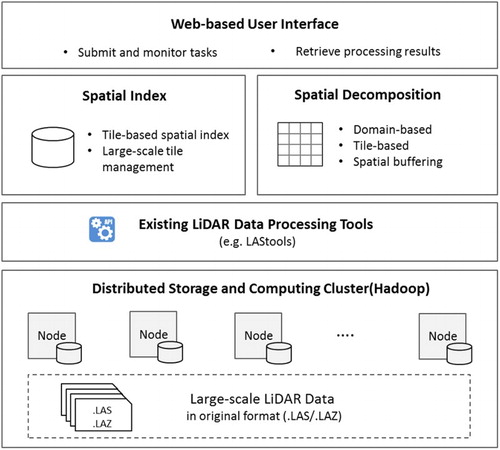
The Distributed Storage and Computing Cluster leverages the de-facto big data processing platform Apache Hadoop to provide both a parallel computing environment as well as the distributed storage system with high-scalability and fault-tolerance.

The Spatial Index (Section 4.2) offers a tile-based indexing approach to associate a tile’s geographic location in the geographic-space to its physical storage location in the computing cluster-space. Enabled by the Spatial Index, large-scale LiDAR data files are stored and managed on the cluster in their original formats (such as .las/.laz)).

The Spatial Decomposition (Section 4.3) component includes two decomposition strategies based on the nature of the processing tasks. Domain-based decomposition is designed for processing tasks that must consider neighboring information, while tile-based decomposition is more efficient when neighboring information is not required.

The Existing LiDAR Data Processing Tools (such as LAStools), that are also designed to work with the .las/.laz format, are configured on each computing node of the cluster, providing native support for conducting various data processing tasks. Bridged by the Spatial Index and Spatial Decomposition, these tools are integrated with MapReduce in a plug-and-play fashion to support parallel data processing (Section 4.4).

An online Web-based User Interface serves as a gateway of the framework for users to submit and monitor LiDAR data processing tasks, and to retrieve the processing result through Hypertext Transfer Protocol (HTTP) (Section 5.1).

4. Methodologies

4.1. Parallel processing of LiDAR data

4.1.1. Tile structure of LiDAR data

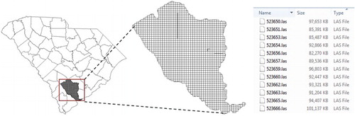
The tile-based structure is widely adopted for storing and managing large-scale LiDAR data. In the tile-based structure, a large spatial area is divided into many regular tiles (normally square) and the data points contained in each tile are stored in one LAS file. A common size tile for county-wide applications is 1524 × 1524 m (5000′ × 5000′). The LAS file format is an industry-standard binary format for storing and interchanging 3D LiDAR (or other) point cloud data (ASPRS 2013). Although originally developed primarily as an interchange format to replace the ASCII de-facto standard, the LAS format has become the native form for many LiDAR processing software applications. Compared to the text-based format (e.g. asci), LAS consumes less storage while delivering higher efficiency for reading and interpreting LiDAR data. Figure 2 shows an example of the tile structure used throughout South Carolina for both LiDAR data and aerial imagery. This tile structure is quite common among the states and counties. For the state-wide LiDAR mapping program in South Carolina, the number of tiles for one of the counties in South Carolina averages 780 with each tile containing about 3.5 million LiDAR returns requiring ∼90 MB storage per tile. A total of 35,896 tiles cover the entire state.

Figure 2. LiDAR data tiles for Colleton County, South Carolina.

Many if not most LiDAR processing software applications use the LiDAR data in the native LAS format. LP360 from QCoherent, FUSION from the US Forest Service, and Environmental Systems Research Institute, Inc. (Esri) use the native LAS structure. Each software application permits the logical grouping (i.e. the LAS Data set, Esri 2016) of LAS files for specific applications (i.e. visualizing and selecting of returns). However, the logical groupings of LAS files, such as the LAS Data set, are designed to manage the tiles in a standalone environment (such as on a single computer) and to be accessed by standalone software tools (i.e. ArcMap), which is not suitable for parallel processing in a distributed environment. To overcome this issue, the HDFS is used in this research as the storage system to manage large-scale LiDAR tiles for two reasons: First, it provides high-scalability and fault-tolerance (Borthakur 2008). Second, it offers native support for processing massive data in parallel with MapReduce.

4.1.2. Tile-level parallelization

Parallel processing of large-scale LiDAR data (i.e. tens of thousands of tiles) can be achieved from different levels following the standard divide-and-conquer strategy in parallel computing. A traditional parallelization approach is to divide a massive number of LiDAR data points (i.e. a LAS file normally stores millions of data points) into many subsets to be handled by multiple processors. We call it point-level parallelization. Significant amounts of effort have been invested to develop task-specific point-level parallelization algorithms (e.g. generating a DEM) by leveraging multi-core CPU or GPU as reviewed in Section 2.

In this framework, we propose a tile-level parallelization mechanism to process a large number of tiles in parallel using the tile as the basic parallelization unit. With tile-level parallelization, we decompose the large number of tiles for a study area into many subdomains, with each subdomain containing one or many tiles. These subdomains are processed with existing standalone LiDAR tools by multiple computers in parallel. For a computing cluster of N computer nodes with each node having M parallel threads (i.e. M CPU cores), a tile-level parallelization is designed to follow three general rules: (1) divide the study area into N*M subdomains with each subdomain containing the same amount of tiles (maximize load balancing), (2) each parallel thread process one subdomain so the N*M subdomains are processed in parallel (maximize parallelization), and (3) each subdomain is processed on the computer node where all or most tiles of the subdomain are stored (maximize data locality).

The tile-level parallelization mechanism is extremely suitable for the popular tile-based structure. Different from point-level parallelization which is task-specific, tile-level parallelization is task-independent since the processing task can be handled by existing LiDAR software modules/tools, such as LAStools and libLAS (http://www.liblas.org). The following subsections elaborate the essential techniques including spatial index, spatial decomposition/scheduling, and job description schema for implementing the tile-level parallelization.

4.2. Spatial index

HDFS offers a highly scalable storage which is important for managing and processing large-scale LiDAR data. However, when storing LAS tiles in HDFS, only the tile names are known. The metadata information for each tile, such as the spatial location of the tile, important for implementing tile-level parallelization, is not available. For example, to follow the first rule, we need to know the geographic location of each tile in HDFS; that is where a tile is located in the study area. For the third rule, we need to know the storage location of each tile in HDFS; that is on which computer node a tile is stored in the cluster.

To facilitate this, a tile-based spatial index is proposed to associate the tile name with the tile’s geographic location and storage location (Figure 2). This index contains the four fields TileName, CentroidX, CentroidY, and LocalNodes. The TileName is the file name of the tile serving as the reference in the file-space. The geographic location of a tile is recorded as the tile’s centroid coordinates (CentroidX, CentroidY), serving as the reference in the geographic-space. When loading tiles into HDFS, each tile is by default replicated to three copies with each copy stored on three different computer nodes. Data replication is used by HDFS to reliably store very large data files across computers in a large cluster (Borthakur 2013). The replication factor can be configured when loading data to HDFS, normally a higher replication factor improves fault-tolerance but requires larger storage. When the replication factor is set to one, the data will not be replicated. The proposed index works with any replication factor. LocalNodes maintains a list of the computer nodes on which a tile is stored, serving as the reference in the cluster-space. In Figure 3, for example, tile T_i is stored on both Node 2 and Node k.

Figure 3. Structure of the tile-based spatial index linking a tile’s (T_i) file-space, geographic-space, and cluster-space.

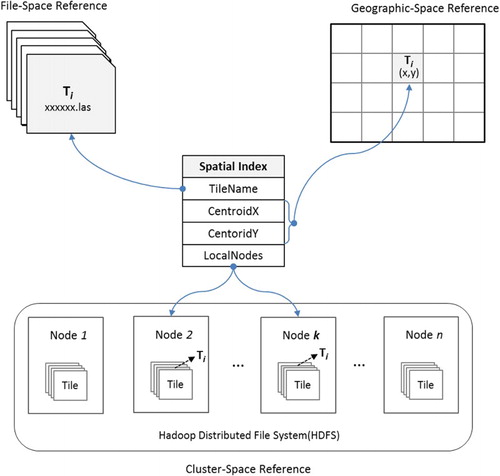
The index is initially built when loading LiDAR tiles into the HDFS, and is stored in a relational database (i.e. MySQL) as a table for fast query and access. Since each index record is independent, the index will be progressively updated by appending new records (without affecting other records) when new tiles are loaded to the HDFS. Since Hadoop HDFS might automatically re-distribute data files (tiles) between nodes to obtain a balanced storage when faced with unexpected node failures, under such circumstances a program will be invoked to synchronize and update information between the index database and the tiles stored in HDFS.

Such a tile-based indexing mechanism provides two key functions for spatial decomposition. First, given a tile name, the tile data can quickly be located on which computer node this tile is stored in the cluster-space (e.g. the set of computer nodes) and where this tile is located in geographic-space. Second, given a spatial region such as a bounding box (bbox), all tiles contained in the region and where these tiles are stored on the cluster is quickly known.

4.3. Spatial decomposition

Two spatial decomposition/scheduling mechanisms are introduced to handle different data processing scenarios following the three rules in the tile-level parallelization.

4.3.1. Domain-based decomposition

Domain-oriented decomposition considers each subdomain as an equal-sized square area represented as a bbox. For a cluster with N*M parallel threads and a study area containing T tiles, the decomposition goal is to create N*M subdomains where each subdomain contains T/(N*M) tiles to achieve good parallelization and load balancing.

Since the subdomain is square shaped, the width (or height) of each subdomain (W_subdomain) can be calculated with Equation 1:(1) where, T denotes number of tiles, N denotes number of nodes, M denotes number of threads per node, and w_tile denotes the width of a tile (assuming the size of the tiles is the same for the study area).

Once the subdomain width is computed, the coordinates of each subdomain (represented as a bbox) can be calculated based on the coordinates of the study area (Figure 4). In most cases, such calculation will result in more than N*M subdomains because the width (or height) of the study area often cannot be divided exactly by the subdomain width. As a result, some subdomains will actually contain a partial number of tiles, we call such subdomain as a partial subdomain (i.e. subdomain B). These partial subdomains are combined to produce N*M subdomains. For example, partial subdomain B can be combined with subdomain C to form a full subdomain.

Figure 4. Illustration of domain-based spatial decomposition.

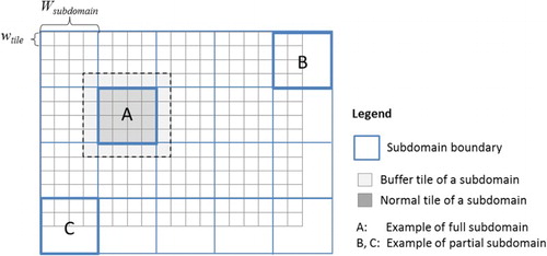
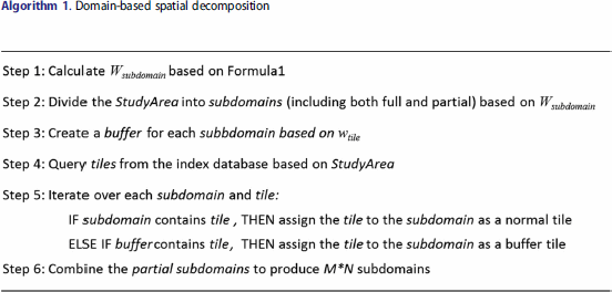
Using subdomains (i.e. points or tiles) that are defined geographically assumes the application does not need spatially adjacent data for the application. However, processing spatial data often requires considering neighboring information; necessitating the spatial data for the node to have continuous spatial coverage. For example, creating a DEM from pseudo-random points (as in LiDAR) requires neighboring points for interpolation of each cell value. A one-tile neighborhood size is clearly adequate for the neighborhood. In this paper, we create a one-tile buffer (the light shaded area) around each subdomain (dark shaded area) as illustrated in Figure 4. All tiles in a subdomain (the dark shaded area) have adjacent tiles when generating a DEM. With this buffering approach, applications involving spatial dependencies (e.g. a very close neighborhood) have an adequate overlap of data containing neighborhood information and thus, the output will not be different from a non-parallel version. The overall logic of the domain-based spatial decomposition is illustrated with Algorithm 1.

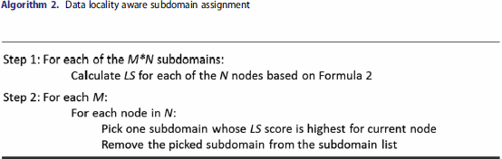
Once the subdomains are created, each node should process M subdomains. An easy way to do this is to assign M subdomains to each node randomly. This approach is not recommended because, for example, if most of the tiles in subdomain A are stored in Node x but subdomain A is assigned to Node y, then Node y needs to read most of the tiles from Node x, causing unnecessary data communication over the network, thus impairing the performance. Therefore, data locality, an important algorithm design principle in the Hadoop environment, should be carefully considered for subdomain assignment. To implement the data locality aware assignment, a data locality score (LS) for a subdomain is defined as Equation 2:(2) where, LS_i denotes data locality score of the subdomain for computer node i; k_i is the number of tiles in this subdomain that are stored on node i; and K is the total number of tiles in this subdomain.

The LS values range from 0 to 1 inclusive where higher scores indicate higher data locality, and thus, less data communication. When calculating LS, the key information is a tile’s local node list which can be rapidly retrieved from the index database. Based on the data LSs, the subdomain assignment procedure is explained in Algorithm 2. Since we assume the size of the tiles is essentially constant for all tiles in the study area in Equation 1, tiles with different sizes cannot be processed as efficiently when using domain-based decomposition.

4.3.2. Tile-based decomposition

Domain-based decomposition provides a general decomposition approach for processing LiDAR tiles in parallel. Since the data locality is a constraint within a subdomain, the LS score is relatively low with the highest score around 0.31 in our testing environment. For some data processing tasks such as the vector to raster conversion or converting between file formats, the tiles can be processed independently without considering neighboring points. Under such scenarios, the geographic location of a tile is no longer needed, and the tile-based decomposition is used to achieve high data locality.

For a cluster with N computing nodes and a study area containing T tiles, the first approximation for a balanced load is to assign T/N tiles to each node considering data locality. During this assigning procedure, we want to make sure that for each node the assigned tiles are physically stored on this node. Li et al. (2017) describe a Grid Assignment strategy to group a large number of climate data grids based on grid storage location in HDFS. In the present study, we adopted the Grid Assignment strategy to achieve data locality. The second step splits the T/N tiles on each node into M groups (subdomains), producing N*M subdomains with each subdomain containing T/(M*N) tiles. Because tile-based decomposition does not consider the tile size, tiles with different sizes can be processed at the same time using a single job.

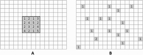
For the same study area, both domain-based and tile-based decomposition produce the same number of subdomains (M*N) with each subdomain having approximately the same number of tiles (T/(M*N)). However, the distribution of the subdomain tiles produced by the two decomposition mechanisms is different. Figure 5 illustrates the hypothesized distribution of 16 tiles (shaded cells) of one subdomain under the two different decomposition scenarios. Figure 5(A) depicts domain-based decomposition scenario where all 16 tiles are spatially close to each other in the geographic-space, but they are stored across different nodes in the cluster-space. The subdomain is assigned to node2 since this subdomain has the highest LS score (5/16 = 0.3125) on node2. Figure 5(b) depicts the tile-based decomposition scenario where most of the tiles in the subdomain are stored on node1 (close to each other in the cluster-space), but they are spatially dispersed. This subdomain is processed on node1 to achieve high data locality (LS score = 15/16 = 0.9375 in this hypothesized case).

Figure 5. The distribution of the subdomain tiles in geographic-space and cluster-space with the two different decomposition mechanisms: (A) domain-based decomposition and (B) tile-based decomposition.

Note: The number in each tile (cell) indicates the computer node that tile is stored (i.e. 1 means the tile is stored on node1).

4.4. Integration with MapReduce and LAStools

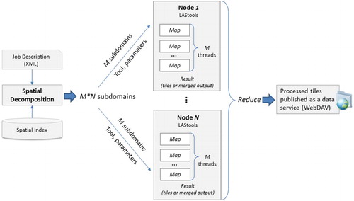
Spatial decomposition (either domain-based or tile-based) decomposes the tiles in the study area into M*N subdomains. Each of the N computer nodes processes M subdomains in parallel by invoking corresponding LiDAR data processing applications (e.g. LAStools), which are installed on each node. A MapReduce program is used to perform the map tasks on each node by (1) loading the subdomain tiles from HDFS and (2) processing them with the existing tools (e.g. use las2dem to generate a DEM) based on the task and parameters specified by the user through a Job Description file. Finally, a reduce task collects all processed tiles and publishes them as a data service using the Web Distributed Authoring and Versioning (WebDAV) (Figure 6); thus, allowing the processed tiles to be accessed and further processed such as mosaicking into a large geographic area using ArcGIS.

Figure 6. Integrating spatial decomposition with MapReduce and LAStools to implement tile-level parallelization.

Note: A Map in this figure refers to the map function of MapReduce.

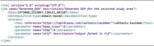
LAStools contains over twenty tools where each tool requires unique parameters and associated values. To enable users to define a processing task in a flexible and reusable way, a Job Description schema is introduced. The schema is encoded with EXtensible Markup Language (XML) as exemplified in Figure 7. The bbox field specifies the process area for this task, which can be used to subset a large geographic area. The decomposition-type indicates the spatial decomposition method to be used (i.e. either domain-based or tile-based). The process contains (1) a tool element to specify the tool used for this process and (2) a varying number of parameters and their values for this process. The parameters of the process match the parameters used in the native LAStools command lines. The input for the process does not need to be specified in the job description file since they are determined based on the spatial decomposition.

Figure 7. An example of the XML-based Job Description.

5. Implementation and evaluation

5.1. Prototype implementation

A proof-of-concept prototype was implemented to evaluate the feasibility, performance, and scalability of the proposed framework. The prototype is powered by a Hadoop cluster (version 2.6.0) consisting of 11 computer nodes (1 master node, 10 computing nodes) connected with 1 Gigabit Ethernet (Gbps). Each node is configured with four physical CPU cores (Intel(R) Xeon(R) CPU E3–1231 v3 @ 3.40 GHz) and 32 GB RAM running on CentOS 6.7. LAStools was installed on each slave node of the cluster. A MySQL database was deployed on the master node of the cluster to manage the tile-based index (generated during the data loading process). While MySQL was used in this prototype, other databases such as PostgreSQL are compatible. An online web-based application was developed serving as the user interface of the prototype (Figure 8). This web application communicates with the Hadoop cluster through HTTP and is deployed on a separate web server but within the same rack (1 Gigabit connection to the cluster nodes).

Figure 8. The online user interface of the prototype and the tile boundaries (red rectangles) of the LiDAR data for Colleton County in South Carolina.

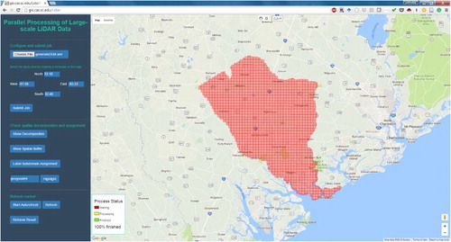
LiDAR data for Colleton County in South Carolina was used as the experimental data. The data are from the state-wide LiDAR data mapping program contained 1378 tiles and 4.17 billion points (∼110 GB in LAS format). The tiles in LAS format were directly loaded to HDFS without any preprocessing. The tile-based spatial index was built during the data loading process and was stored in the MySQL database. The boundary of these LiDAR tiles are displayed on an interactive map (powered by Google Maps, Figure 8). The user can specify a process area by drawing a bbox on the map, which provides an efficient way to subset the data from a large data set. The processing job can be submitted by uploading the Job Description file. The bbox specified in the file will be overwritten by the bbox, if selected, on the map. The processing results will be collected from the 10 computing nodes to the web server, and published as a data service using WebDAV.

5.2. Feasibility evaluation

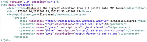
We conducted two types of representative operations against the experimental data using the prototype system. The first operation renders the LiDAR points onto a raster for each tile using the lasgrid tool (gridding operation, https://rapidlasso.com/lastools/lasgrid). A tile-based decomposition strategy was utilized for this operation because these tiles are processed independently without neighboring information (Figure 9). The second operation (DEM operation) generates a DEM using the blast2dem tool (https://rapidlasso.com/blast/blast2dem). A domain-based decomposition strategy was used for this operation to consider spatial dependencies. The lasgrid and blast2dem tools are precompiled executable files widely distributed and used by members of the LiDAR community. Use of these tools requires no coding or compilation.

Figure 9. Job description file for the gridding operation.

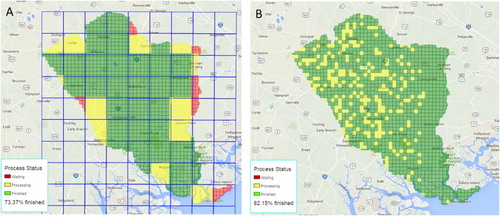
The progress of the task is displayed dynamically online in a map form (Figure 10). The processing status of each tile is represented by colors, and the overall job progress is shown as a percentage (bottom left corner). The status is updated in real time. A snapshot job status of generating a DEM using domain-based decomposition and rasterizing tiles using tile-based decomposition with the experimental data are shown in Figure 10(A) and (B), respectively.

Figure 10. Snapshot of the job status: (A) generating DEM with domain-based decomposition (blue rectangles represent subdomains) and (B) rasterizing tiles with tile-based decomposition.

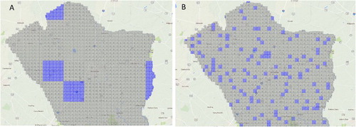
The actual subdomain assignment status of a job can also be monitored on the map as illustrated in Figure 11. The node id of the cluster is displayed in each tile. Figure 11(A) shows the assignment status of the DEM operation (domain-based decomposition). All tiles being processed on node 7 are highlighted in blue. Figure 11(B) shows assignment status of the gridding operation (tile-based decomposition) with tiles being processed on node 7 highlighted. As can be seen, for tile-based decomposition the tile distribution more dispersed in the geographic-space, but most of them (96.3% in this case) are stored on node 7 which mean they are closer to each other in the cluster-space.

Figure 11. Subdomain assignment status for the two jobs with node7 highlighted: (A) generating DEM with domain-based decomposition and (B) rasterizing tiles with tile-based decomposition.

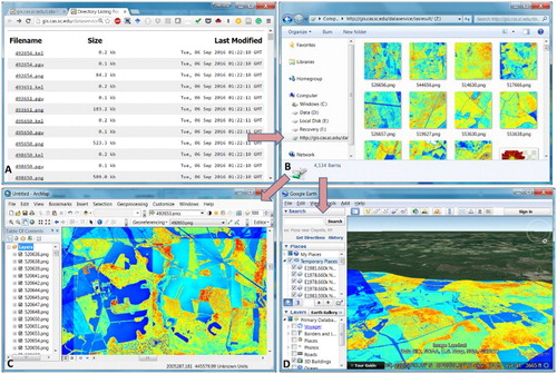
The processing results were automatically collected from the 10 computing nodes to the web server and published as a data service (WebDAV) which can be downloaded through HTTP (Figure 12(A)). By mapping the data service Uniform Resource Locator as a computer Network Drive (Figure 12(B)), the processing results can be directly manipulated with existing software tools, such as using ArcMap to perform further process (Figure 12(C)) or using Google Earth to overlay the images to the terrain (Figure 12(D)).

Figure 12. Manipulation of the results: (A) publishing the processed tiles as a data service; (B) mapping the data service to a computer Network Drive; (C) loading the processed tiles into ArcMap to conduct further process such as mosaic; and (D) displaying the processed tiles in Google Earth. (Note that the tiles displayed in ArcMap and Google Earth are not yet seamlessly mosaicked, so the color discontinuity exists between different tiles from different class intervals.)

5.3. Performance and scalability evaluation

Four experiments were designed to evaluate the system performance and scalability from different aspects by performing the two operations under different scenarios.

5.3.1. Comparison with standalone tools

In this experiment, each operation was conducted on both a standalone computer with traditional LAStools installation and the prototype system (cluster) consisting of 11 computers. All computers have the same hardware specification and operation system as described in Section 5.1. The results are shown in Table 1 illustrating that the cluster system significantly reduces the processing time for both operations. For the DEM operation, the standalone tool required over one hour (3897 seconds) to process 1378 tiles, while the cluster completed in ∼ 12 minutes (723 seconds) producing the same results. Similarly, ∼ 40 minutes (2423 seconds) were required to grid these tiles with the standalone tool, but only 4.4 minutes (261 seconds) with the cluster system. The speedup of using the cluster (denoted as S) for both operations was calculated (Equation 3) using the standalone-time (T_s) divided by the cluster-time (T_c). The results are shown in Table 1:(3) For the gridding operation, the 11-computer cluster (with ten computing nodes) archived a good speedup of 9.28 comparing to the standalone tool, while the speedup for the DEM operation was only 5.38. Such difference primarily results from the consideration of neighboring tiles and the data locality as discussed before. For using the cluster for DEM generation, the spatial buffer for each subdomain needed as illustrated in Figure 4, which causes more tiles to be downloaded and processed than the gridding operation. The gridding operation, on the other hand, processed the same amount of tiles as the standalone scenario. In addition, the gridding operation used the tile-based decomposition, thus resulting in a high data locality. It should be noted that since the standalone LAStool supports multi-core parallelization, it utilized the four CPU cores of a computing node in our test. The prototype system further enabled the parallelization with multiple computing nodes, and the maximum speedup (compared with standalone LAStool) using 10 computing nodes is 10 with 10 computing nodes.

Table 1. Processing time (in second) for the two operations.

	Standalone	Cluster	Speedup
Gridding operation	2423	261	9.28
DEM operation	3891	723	5.38

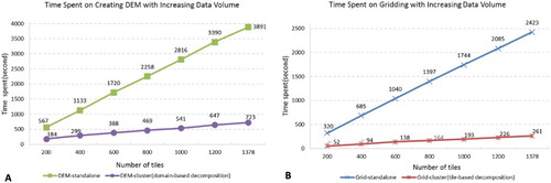
5.3.2. Varying data volume

The effects of varying data volume were also tested. Seven study areas were selected from the experimental data set and the number of tiles (indicating data volume) for each study area increased gradually from 200 to 1378. For each study area, the two operations described in Section 5.2.1 are performed using both the cluster system and the standalone tool.

The results are shown in Figure 13. For both operations performed on the cluster, the time increased proportionally with the increase of data volume, which indicates that the system scales well with the increasing workload. Not surprisingly, for the standalone tool, the time spent on the two operations showed a similar linear pattern but with a much steeper slope. The time difference between the standalone tool and the cluster increased drastically when the data volume increased.

Figure 13. Time spent on the two operations using both the standalone tool and the cluster system when gradually increasing the data volume from 200 to 1378 tiles.

Note: For the case of 1378 tiles, the previous results were used.

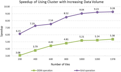
To further explore the influence of data volume we calculated the speedup (Equation 3) of using the cluster system for each operation and study area. As demonstrated in Figure 14, the speedup increases as the data volume increase for both operations. For gridding, we observed a 6.15 speedup when processing 200 tiles, and this number rose to 9.28 when processing the entire1378 tiles covering Colleton county. For the DEM generation, the lowest speedup (3.08) occurred with 200 tiles, and highest (5.38) occurred at the full 1378 tiles. This result indicates that the prototype system is more efficient when handling larger data sets. This is reasonable because when the data volume is small, the system overhead accounts for a larger portion of the total time.

Figure 14. Speedup of using the prototype when gradually increasing the data volume for both operations.

5.3.3. Varying number of nodes

In this experiment, we tested the system scalability by increasing the number of computing nodes from 1 to 10 to conduct the gridding operation using the tile-based decomposition strategy. We conducted the test for three study areas (100, 600, and 1378 tiles) to explore how the scalability differs when processing different data volumes.

Not surprisingly, the processing time for all three study areas decreased when increasing the number of computing nodes (Figure 15(A)). The study area with 1378 tiles showed the most significant decrease in processing time and dropped from 2002 seconds with one computing node to 251 seconds with 10 nodes. For the study area with 100 tiles, the time dropped from 193 to 37 seconds. This result indicates that the system scales well when adding more computing nodes. To better explore this, we again calculated the speedup with Equation 4:(4) where denotes the speedup with n computing nodes. denotes the time using one computing nodes. denotes the time using n computing nodes. Different from Equation 3 where the baseline was the time for standalone tools, the baseline in Equation 4 is the time spent when the cluster only consists of one computing node (and one master node).

Figure 15. Time spent on gridding operation (A) and its corresponding speedup (B) with different number of nodes under different data volume scenarios.

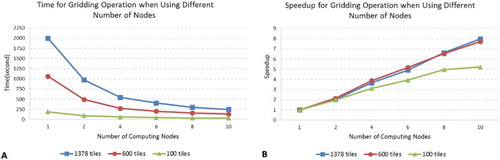
As illustrated in Figure 15(B), the system shows almost linear scalability when processing relatively larger data volumes, with the highest speedup (7.71 for 600 tiles and 7.97 for 1378 tiles) achieved with 10 computing nodes. For the small data volume scenario (100 tiles), the speedup leveled off at eight computing nodes. These results are consistent with the previous discussion that when data volume is small, the system overhead accounts for a major portion of the time consumed.

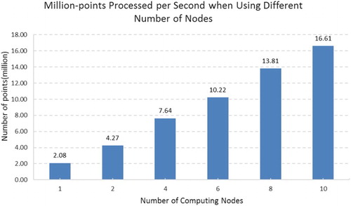
To further demonstrate the system scalability, we calculated the number of points that are processed per second for the 1378-tile scenario. As illustrated in Figure 16, with every two nodes added, the system processed about 3 million more points per second. When using 10 computing nodes, the system processed 16.61 million points per second for the gridding operation.

Figure 16. Number of points processed per second when conducting gridding operation for 1378 tiles.

5.3.4. Comparing decomposition strategies

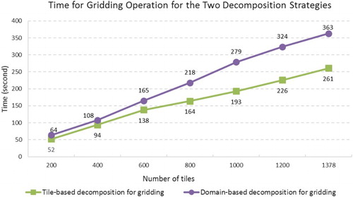
As discussed in Section 4.3.2, for tasks that are not spatially dependent, tile-based decomposition is more efficient than domain-based decomposition because tile-based decomposition typically results in higher data locality. To test this, we conducted the gridding operation for the seven study areas using both tile-based and domain-based decomposition using the prototype (10 computing nodes).

Results show that tile-based composition delivered higher performance (less time) for all study areas (Figure 17), which is consistent with our previous observations. In this experiment, the data LS with tile-based decomposition normally reached 0.9, while the score for domain-based decomposition was around 0.3. This result demonstrates that the characteristics of different data processing tasks are important for designing efficient spatial decomposition algorithms.

Figure 17. Comparison of tile-based decomposition and domain-based decomposition.

6. Conclusion and discussion

A general-purpose framework was proposed to efficiently process large-scale LiDAR point cloud data in parallel in a highly scalable distributed environment by leveraging Hadoop and existing LiDAR processing tools. The feasibility of the proposed framework is demonstrated with a proof-of-concept prototype system. The LAStools were used as the exemplary LiDAR tools due to their high popularity and efficiency. The performance and scalability were evaluated with a series of experiments conducted on a real LiDAR data set. The results show that the proposed parallel processing approach dramatically reduces processing time and thus, allows for greater experimentation with parameter values in each application. The implemented prototype demonstrates how a distributed LiDAR parallel processing environment could be presented as an online geoprocessing application through a web-based map application. Finally, the framework demonstrates software reusability in that (1) existing compiled tools are incorporated – no unique application coding is required and (2) the existing data structure (e.g. .las) of large geospatial data sets was incorporated – no need to import and reformat into a custom data structure.

Decomposition and locality are two important issues for parallel processing of geospatial data, especially in a distributed environment (Armstrong 2010; Yang et al. 2016). For example, Wang and Armstrong (2003) and Wang, Cowles, and Armstrong (2008 ) proposed an approximation to locality-based decomposition to minimize data starvation and communication latency. The two spatial decomposition methods proposed in this paper consider the data locality and geographic relationships to minimize data communication among computer nodes. In addition, different data processing scenarios may have unique characteristics/requirements (e.g. whether to involve neighboring tiles). This paper demonstrates that honoring such differences is important for designing efficient spatial decomposition mechanisms. For processes that must consider spatial relationships, proximity in both the geographic-space and the cluster-space should be considered. For processes that are not spatially dependent, proximity in the cluster-space is the major guideline to maximize data locality. We believe such observations provide a valuable reference for other similar studies seeking to leverage Hadoop or other similar distributed computing platforms for processing geospatial big data.

The proposed framework has some limitations. Future research is required to improve the framework and the prototype system as suggested below:

• While domain-based decomposition uses a data locality aware assignment strategy, the LS only reaches around 0.3 in our experiment. The low data locality impairs the performance as demonstrated in Section 4.3.2. A potential solution for this issue is to investigate a new data placement strategy by considering tile proximity in both geographic-space and cluster-space. Such a placement strategy needs to ensure that, when loading LiDAR tiles to HDFS, tiles that are spatially close to each other are stored on the same machine.

• A LiDAR data processing task may be composed of one or more processes in a workflow style to produce the final product. Taking DEM generation as an example, depending on the level of original LAS tiles, it may first be required to classify the data points into ground points and non-ground points, and subsequently generate a DEM. The ability to chain a set of tools to support such a workflow-style processing is desirable.

• Cloud computing and virtualization technologies provide on-demand and scalable computing resources which have been widely adopted for supporting a variety of geospatial studies. Exploring the feasibility of the proposed framework in a cloud computing environment, such as Amazon Elastic MapReduce, is desirable.

Global concerns (e.g. climate change) call for collaborative data and computing infrastructures for discovering, sharing, and processing the ever growing big geospatial data (Li et al. 2011; Yang et al. 2011). GIScience initiatives such as the geospatial Cyberinfrastructure (Yang et al. 2010; Wright and Wang 2011) and CyberGIS (Wang 2010) aim to meet such demands by combining geospatial data, computing platforms, computational services, and network protocols for better supporting Digital Earth and related geospatial studies. The proposed framework provides one approach on developing such a collaborative infrastructure for processing big LiDAR data in a highly scalable environment.

Acknowledgements

We thank the three anonymous reviewers for their insightful comments that greatly improved the manuscript.

Disclosure statement

No potential conflict of interest was reported by the authors.

ORCID

Zhenlong Li http://orcid.org/0000-0002-8938-5466

Additional information

Funding

This study was funded by University of South Carolina through the ASPIRE (Advanced Support for Innovative Research Excellence) program [13540-16-41796]. Additional funding was provided by the South Carolina Department of Transportation under contract to the University of South Carolina [SPR #707 or USC 13540FB11], USGS [G15AC00085], and NSF-BCS [1455349].

References

- Aljumaily, H., D. F. Laefer, and D. Cuadra. 2015. “Big-data Approach for Three-dimensional Building Extraction from Aerial Laser Scanning.” Journal of Computing in Civil Engineering, 30 (3). doi:10.1061/(ASCE)CP.1943-5487.0000524
- Armstrong, M. P. 2010. “Exascale Computing, Cyberinfrastructure, and Geographical Analysis.” In 2010 NSF Cyber-GIS workshop Washington, DC, February 2–3.
- ASPRS. 2013. “LAS Specification Version 1.4 – R13 15 July 2013.” Accessed September 5, 2016. http://www.asprs.org/wp-content/uploads/2010/12/LAS_1_4_r13.pdf.
- Borthakur, D. 2008. “HDFS Architecture Guide.” Accessed September 5, 2016. http://hadoop.apache.org/common/docs/current/hdfsdesign.pdf.
- Borthakur, D. 2013. “HDFS Architecture Guide.” Accessed September 5, 2016. https://hadoop.apache.org/docs/r1.2.1/hdfs_design.html.
- Bui, G., P. Calyam, B. Morago, R. B. Antequera, T. Nguyen, and Y. Duan. 2015. “LIDAR-based Virtual Environment Study for Disaster Response Scenarios.” In 2015 IFIP/IEEE international symposium on Integrated Network Management (IM), Ottawa, Canada, May 11–15, 790–793. IEEE.
- Crosby, C., J. Arrowsmith, V. Nandigam, and C. Baru. 2011. “Online Access and Processing of LiDAR Topography Data.” In Geoinformatics: Cyberinfrastructure for the Solid Earth Sciences, edited by G. Keller and C. Baru, 251–265. Cambridge: Cambridge University Press. doi:10.1017/CBO9780511976308.017.
- Dean, J., and S. Ghemawat. 2008. “MapReduce: Simplified Data Processing on Large Clusters.” Communications of the ACM 51 (1): 107–113. doi: 10.1145/1327452.1327492
- Esri. 2016. “What is a LAS Dataset?” Accessed July 13, 2016. http://desktop.arcgis.com/en/arcmap/10.3/manage-data/las-dataset/what-is-a-las-dataset-.htm.
- Goetz, S. J., D. Steinberg, M. G. Betts, R. T. Holmes, P. J. Doran, R. Dubayah, and M. Hofton. 2010. “LiDAR Remote Sensing Variables Predict Breeding Habitat of a Neotropical Migrant Bird.” Ecology 91 (6): 1569–1576. doi: 10.1890/09-1670.1
- Guan, H., J. Li, L. Zhong, Y. Yongtao, and M. Chapman. 2013. “Process Virtualization of Large-scale LiDAR Data in a Cloud Computing Environment.” Computers & Geosciences 60: 109–116. doi: 10.1016/j.cageo.2013.07.013
- Guan, X., and H. Wu. 2010. “Leveraging the Power of Multi-core Platforms for Large-scale Geospatial Data Processing: Exemplified by Generating DEM from Massive LiDAR Point Clouds.” Computers & Geosciences 36 (10): 1276–1282. doi: 10.1016/j.cageo.2009.12.008
- Han, S. H., J. Heo, H. G. Sohn, and K. Yu. 2009. “Parallel processing method for airborne laser scanning data using a PC cluster and a virtual grid.” Sensors 9 (4): 2555–2573. doi: 10.3390/s90402555
- Hanusniak, V., M. Svalec, J. Branicky, L. Takac, and M. Zabovsky. 2015. “Exploitation of Hadoop Framework for Point Cloud Geographic Data Storage System.” 2015 fifth International Conference on Digital Information Processing and Communications (ICDIPC), Sierre, Switzerland, October 7–9, 197–200. IEEE.
- Hodgson, M. E., and P. Bresnahan. 2004. “Accuracy of Airborne LiDAR-derived Elevation: Empirical Assessment and Error Budget.” Photogrammetric Engineering & Remote Sensing 70 (3): 331–339. doi: 10.14358/PERS.70.3.331
- Hodgson, M. E., Y. Cheng, P. Coleman, and R. C. Durfee. 1995. “GIS Computational Burdens: Solutions with Heuristic Algorithms and Parallel Processing.” GeoInfo Systems 4: 28–37.
- Homm, F., N. Kaempchen, J. Ota, and D. Burschka. 2010. “Efficient Occupancy Grid Computation on the GPU with LiDAR and Radar for Road Boundary Detection.” In Intelligent Vehicles symposium (IV), Sofitel Gold Coast Broadbeach, Gold Coast City, Australia, June 23–26, 1006–1013. IEEE.
- Hu, X., X. Li, and Y. Zhang. 2013. “Fast Filtering of LiDAR Point Cloud in Urban Areas Based on Scan Line Segmentation and GPU Acceleration.” IEEE Geoscience and Remote Sensing Letters 10 (2): 308–312. doi: 10.1109/LGRS.2012.2205130
- Huang, F., D. Liu, X. Tan, J. Wang, Y. Chen, and B. He. 2011. “Explorations of the Implementation of a Parallel IDW Interpolation Algorithm in a Linux Cluster-based Parallel GIS.” Computers & Geosciences 37 (4): 426–434. doi: 10.1016/j.cageo.2010.05.024
- Hug, C., P. Krzystek, and W. Fuchs. 2004. “Advanced LiDAR Data Processing with LasTools.” In XXth ISPRS Congress, Istanbul, Turkey, July 12–23, 12–23.
- Isenburg, M. 2012. “LAStools-efficient Tools for LiDAR Processing.” Accessed June 16, 2016. http: http://www.cs.unc.edu/~isenburg/lastools.
- Kersting, J., and A. P. B. Kersting. 2005. “LIDAR Data Points Filtering using ArcGIS’3D and Spatial Analyst.” In proceedings of the 25th ESRI user conference, San Diego, CA, July 25–29.
- Kwan, M. P., and D. M. Ransberger. 2010. “LiDAR Assisted Emergency Response: Detection of Transport Network Obstructions Caused by Major Disasters.” Computers, Environment and Urban Systems 34 (3): 179–188. doi: 10.1016/j.compenvurbsys.2010.02.001
- Lausten, K. 2007. “ENVI LiDAR Toolkit. Technical Report.” Accessed June 15, 2016. http://exelis.http.internapcdn.net/exelis/pdfs/2-13_ENVILiDAR_Brochure_LoRes.pdf.
- Li, Z., F. Hu, J. L. Schnase, D. Q. Duffy, T. Lee, M. K. Bowen, and C. Yang. 2017. “A Spatiotemporal Indexing Approach for Efficient Processing of Big Array-based Climate Data with MapReduce.” International Journal of Geographical Information Science 31 (1): 17–35. doi: 10.1080/13658816.2015.1131830
- Li, J., Y. Jiang, C. Yang, Q. Huang, and M. Rice. 2013. “Visualizing 3D/4D Environmental Data Using Many-core Graphics Processing Units (GPUs) and Multi-core Central Processing Units (CPUs).” Computers & Geosciences 59: 78–89. doi: 10.1016/j.cageo.2013.04.029
- Li, Z., C. Yang, B. Jin, M. Yu, K. Liu, M. Sun, and M. Zhan. 2015. “Enabling Big Geoscience Data Analytics with a Cloud-based, MapReduce-enabled and Service-oriented Workflow Framework.” PloS One 10 (3): e0116781. doi: 10.1371/journal.pone.0116781
- Li, Z., C. Yang, K. Liu, F. Hu, and B. Jin. 2016. “Automatic Scaling Hadoop in the Cloud for Efficient Process of Big Geospatial Data.” ISPRS International Journal of Geo-Information 5 (10): 173–191. doi: 10.3390/ijgi5100173
- Li, Z., C. P. Yang, H. Wu, W. Li, and L. Miao. 2011. “An Optimized Framework for Seamlessly Integrating OGC Web Services to Support Geospatial Sciences.” International Journal of Geographical Information Science 25 (4): 595–613. doi: 10.1080/13658816.2010.484811
- Liu, Y. Y., D. R. Maidment, D. G. Tarboton, X. Zheng, A. Yildirim1, N. S. Sazib, and S. Wang. 2016. “CyberGIS Approach to Generating High-resolution Height Above Nearest Drainage (HAND) Raster for National Flood Mapping.” CyberGIS Center technical report, CYBERGIS-TR-2016-005.
- Lopatin, J., K. Dolos, H. J. Hernández, M. Galleguillos, and F. E. Fassnacht. 2016. “Comparing Generalized Linear Models and Random Forest to Model Vascular Plant Species Richness Using LiDAR Data in a Natural Forest in Central Chile.” Remote Sensing of Environment 173: 200–210. doi: 10.1016/j.rse.2015.11.029
- Lukač, N., and B. Žalik. 2013. “GPU-based Roofs’ Solar Potential Estimation Using LiDAR Data.” Computers & Geosciences 52: 34–41. doi: 10.1016/j.cageo.2012.10.010
- Luo, W., and H. Zhang. 2015. “Visual Analysis of Large-scale LiDAR Point Clouds.” 2015 IEEE international conference on Big Data (Big Data), Santa Clara, CA, October 29-November 1, 2487–2492. IEEE.
- Ma, H., and Z. Wang. 2011. “Distributed Data Organization and Parallel Data Retrieval Methods for Huge Laser Scanner Point Clouds.” Computers & Geosciences 37 (2): 193–201. doi: 10.1016/j.cageo.2010.05.017
- McGaughey, R. J. 2009. “FUSION/LDV: Software for LIDAR Data Analysis and Visualization.” US Department of Agriculture, Forest Service. Seattle, WA: Pacific Northwest Research Station, 123(2).
- Neteler, M., M. H. Bowman, M. Landa, and M. Metz. 2012. “GRASS GIS: A Multi-purpose Open Source GIS.” Environmental Modelling & Software 31: 124–130. doi: 10.1016/j.envsoft.2011.11.014
- Oryspayev, D., R. Sugumaran, J. DeGroote, and P. Gray. 2012. “LiDAR Data Reduction Using Vertex Decimation and Processing with GPGPU and Multicore CPU Technology.” Computers & Geosciences 43: 118–125. doi: 10.1016/j.cageo.2011.09.013
- Svanberg, S. 2015. “LiDAR Techniques for Environmental and Ecological Monitoring.” In EGU general assembly conference abstracts, 17, 13357 Vienna, Austria, April 12–17.
- Tarolli, P., J. R. Arrowsmith, and E. R. Vivoni. 2009. “Understanding Earth Surface Processes from Remotely Sensed Digital Terrain Models.” Geomorphology 113 (1): 1–3. doi: 10.1016/j.geomorph.2009.07.005
- Tesfa, T. K., D. G. Tarboton, D. W. Watson, K. A. Schreuders, M. E. Baker, and R. M. Wallace. 2011. “Extraction of Hydrological Proximity Measures from DEMs Using Parallel Processing.” Environmental Modelling & Software 26 (12): 1696–1709. doi: 10.1016/j.envsoft.2011.07.018
- Venugopal, V., and S. Kannan. 2013. “Accelerating Real-time LiDAR Data Processing Using GPUs.” 2013 IEEE 56th international Midwest Symposium on Circuits and Systems (MWSCAS), Columbus, OH, August 4–7, 1168–1171. IEEE.
- Vierling, K. T., L. A. Vierling, W. A. Gould, S. Martinuzzi, and R. M. Clawges. 2008. “LiDAR: Shedding New Light on Habitat Characterization and Modeling.” Frontiers in Ecology and the Environment 6 (2): 90–98. doi: 10.1890/070001
- Wang, S. 2010. “A CyberGIS Framework for the Synthesis of Cyberinfrastructure, GIS, and Spatial Analysis.” Annals of the Association of American Geographers 100 (3): 535–557. doi: 10.1080/00045601003791243
- Wang, S., and M. P. Armstrong. 2003. “A Quadtree Approach to Domain Decomposition for Spatial Interpolation in Grid Computing Environments.” Parallel Computing 29 (10): 1481–1504. doi: 10.1016/j.parco.2003.04.003
- Wang, S., M. K. Cowles, and M. P. Armstrong. 2008. “Grid Computing of Spatial Statistics: Using the TeraGrid for Gi*(d) Analysis.” Concurrency and Computation: Practice and Experience 20 (14): 1697–1720. doi: 10.1002/cpe.1294
- Wright, D. J., and S. Wang. 2011. “The Emergence of Spatial Cyberinfrastructure.” Proceedings of the National Academy of Sciences 108 (14): 5488–5491. doi: 10.1073/pnas.1103051108
- Yang, C., Q. Huang, Z. Li, K. Liu, and F. Hu. 2016. “Big Data and Cloud Computing: Innovation Opportunities and Challenges.” International Journal of Digital Earth, 1–41. doi:10.1080/17538947.2016.1239771.
- Yang, C., R. Raskin, M. Goodchild, and M. Gahegan. 2010. “Geospatial Cyberinfrastructure: Past, Present and Future.” Computers, Environment and Urban Systems 34 (4): 264–277. doi: 10.1016/j.compenvurbsys.2010.04.001
- Yang, C., H. Wu, Q. Huang, Z. Li, and J. Li. 2011. “Using Spatial Principles to Optimize Distributed Computing for Enabling the Physical Science Discoveries.” Proceedings of the National Academy of Sciences 108 (14): 5498–5503. doi: 10.1073/pnas.0909315108
- Yonglin, S., W. Lixin, and W. Zhi. 2010. “Identification of Inclined Buildings from Aerial LiDAR Data for Disaster Management.” In 2010 18th international conference on Geoinformatics, Beijing, China, June 18–20, 1–5. IEEE.
- You, Y., L. Fan, K. Roimela, and V. V. Mattila. 2014. “Simple Octree Solution for Multi-resolution LiDAR Processing and Visualisation.” 2014 IEEE international conference on Computer and Information Technology (CIT), Dhaka, Bangladesh, December 22–23, 220–225. IEEE.
- Youn, C., V. Nandigam, M. Phan, D. Tarboton, N. Wilkins-Diehr, C. Baru, and S. Wang. 2014. “Leveraging XSEDE HPC Resources to Address Computational Challenges with High-resolution Topography Data.” In proceedings of the 2014 annual conference on Extreme Science and Engineering Discovery Environment, Atlanta, GA, July 13–18, 59, CM.
- Zhao, Y., A. Padmanabhan, and S. Wang. 2013. “A Parallel Computing Approach to Viewshed Analysis of Large Terrain Data Using Graphics Processing Units.” International Journal of Geographical Information Science 27 (2): 363–384. doi: 10.1080/13658816.2012.692372