FunnelCloud: a cloud-based system for exploring tornado events

ABSTRACT

Recent research has shown an increase in the number of extreme tornado outbreaks per year. The characterization of the spatio-temporal pattern of tornado events is therefore a critical task in the analysis of meteorological data. Currently, there are a large number of available meteorological datasets that can be used for such analysis. However, much of these data are distributed across multiple websites and are not accessible in a central location. This poses a significant challenge for a scientist who is interested in exploring meteorological patterns associated with tornado events. This paper presents a novel system which uses cloud-based technology for integrating, storing, exploring, analyzing, and visualizing meteorological data associated with tornado outbreaks. The system employs a novel NoSQL database schema and web services architecture for data integration and provides a user friendly interface that allows scientists to explore the spatio-temporal pattern of tornado events. Furthermore, scientists can use this interface to analyze the relationship between different meteorological variables and properties of tornado outbreaks using a number of spatio-temporal statistical and data mining methods. The efficacy of the system is demonstrated on a use case centered on the analysis of climatic indicators of large spatio-temporally clustered tornado outbreaks.

KEYWORDS:

• tornado data warehouse
• cloud-based system
• NoSQL
• data integration
• spatio-temporal clustering
• web-mapping

1. Introduction

Tornadoes are one of the most destructive and unpredictable natural disasters responsible for the loss of life and property. The United States experiences more tornadoes than any other country on Earth (Grazulis 1990). For example, in the year 2015 alone, there were 1178 confirmed tornadoes, which caused 36 fatalities and up to 321 million financial damages. There is little doubt that Earth is in a period of climate change. This climate change can have many impacts including increased storm intensity (Barros et al. 2014). More intense storms could result in an increase in the frequency and intensity of tornado events.

Scientists have invested a great deal of time and resources to study the environmental conditions that contribute to tornado events. This analysis requires a number of disparate data products including tornado touchdown locations, and various meteorological data products from a number of different sources. These data then need to be converted to a suitable format for analysis and visualization. It has been shown that advancements in data assimilation (DA) techniques and forecasting methods can allow for more accurate forecasting of tornado events (Kalnay 2003). However, there is still a great deal to be learned regarding the meteorological and climatic conditions that are favorable for tornado genesis and therefore, new techniques for data integration, analysis, and visualization are needed to allow scientists to explore the relationship between tornadoes and meteorological variables.

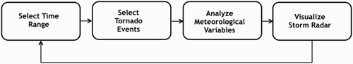
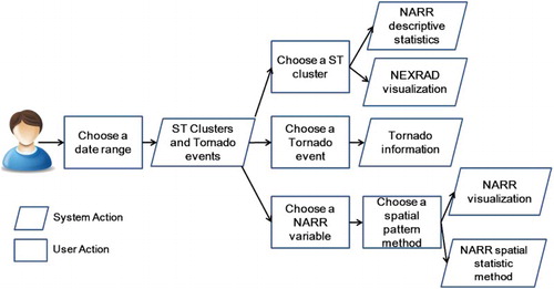
This paper is motivated by a scientific workflow (Figure 1) that allows a scientist to explore meteorological conditions associated with tornado events. The first step is to be able to select an appropriate time range within which a tornado event or series of tornado events occurred. Then, given this time range, the scientist would like to select tornado events of interest based on their location. Once a tornado event is selected, the scientist would like to analyze meteorological variables associated with the location of the tornado event in space and time. Finally, the scientist would also like to explore the spatio-temporal pattern of the Next-Generation Weather Radar (NEXRAD) signature through the visualization of radar data.

Figure 1. Workflow for exploratory analysis of tornado data.

To realize this scientific workflow, a number of datasets need to be integrated. This includes tornado event data from the National Oceanic and Atmospheric Administration/National Climatic Data Centers (NOAA/NCDC) Storm Prediction Center (SPC) (SPC 2016), National Centers for Environmental Prediction (NCEP) North American Reanalysis data from the NOAA/OAR/ESRL (Mesinger et al. 2006), and NEXRAD data from the National Centers for Environmental Information (NEXRAD 2016).

The above workflow results in a massive amount of data where efficient methods for integration and analysis are still a challenge. Recent advances in cloud computing allow these data to be stored in a shared pool and processed in an on-demand fashion (Mell and Grance 2011). This approach provides a number of advantages (Armbrust et al. 2009). First, multiple users from different locations can have access to the data simultaneously. Also, retrieving data from the Internet rather than storing data locally for each scientist saves disk space. Moreover, cloud computing improves system performance because much of the processing can be offloaded to large servers. Finally, when using a distributed database environment, this approach is scalable to very large datasets where new nodes can easily be added to the data center without affecting the associated web services that provide access to the data.

With the above motivation in mind, this paper presents FunnelCloud, a cloud-based system for the analysis of the spatio-temporal pattern of tornado events and their associated environmental conditions. The FunnelCloud system integrates disparate sources of data into a Non Structured Query Language (NoSQL) database system and includes a web services architecture for the analysis and visualization of tornado patterns and related meteorological variables. One of the core functions of the FunnelCloud system is to provide a method for finding spatio-temporal clusters of tornadoes based on a date range supplied by the user. Taking these clusters as an output, scientists can then explore tornado events to analyze tornado patterns with related meteorological variables. The paper is organized as follows: Section 2 presents works related to this research, Section 3 presents the design of the system, Section 4 presents a real-world use case where the system is used for the analysis of a tornado event, and Section 5 provides a conclusion and discussion of the future directions of this research.

2. Related work

The analysis of meteorological data requires a large number of attributes from numerous data sources distributed in space and time. The integration of which can be a time consuming task for scientists. A number of geographic information systems (GIS) have been developed to integrate meteorological data for this purpose. Powell et al. (1998) have designed an objected-oriented, distributed client–server application for storm tracking and wind field analysis. An online climate-related natural hazard vulnerability assessment support system prototype has been created by Coletti et al. (2013). This online environment integrates different data sources and allows users to visualize data and easily discuss the impacts of natural hazards. Camp et al. (2015) developed a seasonal forecast system named GloSea5 to predict tropical storm activity and landfall frequency along the Caribbean coastline. Cox et al. (1995) built an interactive graphical interface-based objective kinematic analysis system to explore wind fields. The system allows an analyst to view and manipulate wind inputs when doing wind field analysis. Maidment (2006) developed a hydrologic information system that contained web services and analysis tools to allow users explore data from different available datasets. Finally, the HydroCloud system has integrated different sources of hydrologic data and provided interactive tools for exploratory data analysis and statistical hypothesis testing (McGuire, Roberge, and Lian 2016). All these previous works indicate that building an integrated geographical data system is useful for scientists to explore and analyze climate patterns efficiently.

Clustering is a data mining approach that has been used to detect spatial and temporal patterns in climate data (Hoffman et al. 2005). Lakshmanan (2001) and Lakshmanan and Smith (2009) have utilized the K-means clustering method to identify high-intensity thunder storm supercells. Spatio-temporal clustering is a relatively new and promising subfield in data mining and has been used for the analysis of climate and meteorological data. In spatio-temporal clustering, objects are classified based on both spatial and temporal similarities.   Strauss, Rosa, and Stephany (2013) developed a spatio-temporal clustering method that uses a sliding window and standard kernel density estimation to analyze the relationship between precipitation intensity and lightning strike locations. Furthermore, Birant and Kut (Birant and Kut 2006) have studied spatio-temporal marine data and developed ST-DBSCAN (Spatio Temporal-Density-Based Spatial Clustering Applications with Noise) clustering algorithm to find seawater regions that have similar physical characteristics.

Recent advances in cloud computing and virtualization technology have brought forth a revolution in the analysis of big data such as that found in the domains of climatology and meteorology (Jansen 2011; Yang et al. 2011). One of the most important challenges in the analysis of these data are that the spatial domain of the climatic system is multi-scale in nature where local meteorological phenomena are affected by large-scale global climatic processes (Steinhaeuser, Ganguly, and Chawla 2012). The analysis of multiple scales of spatial data can be very computationally intensive. With this in mind, using a distributed cloud-based architecture scales well to support these types of analyses. Cloud-based data warehouses have been shown to support data on the petabyte scale (Thusoo et al. 2010) and it is possible to conduct aggregation queries using the MapReduce framework (Brezany et al. 2011; Cao et al. 2011). The use of cloud architectures in geospatial science has been identified as an emerging technology that will extend cloud computing beyond its current technological boundaries (Yang et al. 2011). Most recently, a cloud-based architecture built on Hadoop has shown to be effective in querying spatial dimensions of scientific datasets (Aji and Wang 2012) and medical imaging (Aji, Wang, and Saltz 2012). Document databases such as MongoDB have shown to be very effective in the distributed management of spatial data (Han et al. 2013) and geoanalytic frameworks (Heard 2011). Finally, most related to our proposed tornado system, Dyer and Baugh (2016) provided a graphical interactive user interface that was capable of implementing a subdomain modeling technique to perform hurricane simulations on multiple alternate topographies in a region of interest with less computational cost. However, the computation in this technique is still on the client side, which means it affects performance when facing large calculations on big datasets.

The research presented in this paper builds on the existing literature through the utilization of cloud-based technologies to construct a system for the integration and analysis of data associated with tornado outbreaks. The contributions of this paper can be summarized as follows:

• Extraction, Transformation and Loading (ETL) workflows were developed to integrate spatio-temporal datasets needed for the analysis of tornado events.

• The system was implemented using an NoSQL database technology that is both scalable and efficient.

• A spatio-temporal clustering algorithm was implemented to cluster tornado events based on both the tornado's touch down location and timestamp.

• A web services architecture was developed to provide an extensible framework from which mashups and new applications can be developed.

• A novel map-based visualization was developed to explore radar data as well as a number of meteorological data.

• The system was validated by a real-world case study based on the exploration and analysis of tornado events.

3. The FunnelCloud system

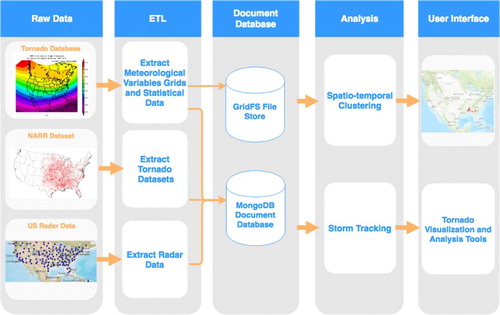
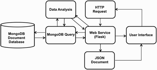
The architecture of the FunnelCloud system is shown in Figure 2. First, a number of tornado-related datasets are integrated from various publicly available data sources to form the FunnelCloud data warehouse. These data are extracted from its source format and transformed into large JavaScript Object Notation (JSON) documents. The documents are then stored in MongoDB, an NoSQL document-oriented database. The database can be accessed through a number of Representational state transfer (RESTful) web services as well as a web-based client for visualization and statistical analysis. The web service API allows the analysis and visualization tools to get different kinds of data efficiently and provides a useful method for other researchers to access the integrated dataset to create their own tools.

Figure 2. Overview of the FunnelCloud system architecture.

The rest of this section will elaborate on the design of the FunnelCloud system where Section 3.1 presents the datasets included in the FunnelCloud data warehouse. Section 3.2 describes the document-oriented database model. Section 3.3 describes the ETL processes that are used to automatically load data into the data model. Section 3.4 describes the spatio-temporal clustering method to find tornado events grouped in space and time. Section 3.5 introduces the design of web services that are used to explore the integrated dataset and Section 3.6 describes the performance of the FunnelCloud system.

3.1. Datasets

The FunnelCloud system contains several heterogeneous data types including geospatial data and metadata. The data sources, summarized in Table 1, include the NCEP NARR meteorological data warehouse (Mesinger et al. 2006), the NOAA SPC tornado event dataset (SPC 2016), the National Weather Service hosted on Amazon Web Service (AWS) (AWS 2016) and Open Geospatial Consortium (OGC) Tile Map Service (TMS) for 8 bit NEXRAD radar base reflectivity (OGC 2016).

Table 1. Data sources for FunnelCloud system.

Dataset name	Data source	Format	Data type
NCEP North American Regional Reanalysis	http://www.esrl.noaa.gov/psd/data/gridded/data.narr.html	NetCDF	Gridded geospatial data
NOAA SPC	http://www.spc.noaa.gov/gis/svrgis/	CSV	Metadata, geographic points
NEXRAD on Amazon Web Service	https://aws.amazon.com/noaa-big-data/nexrad/	Web service	Gridded geospatial data
Open Geospatial Consortium	https://mesonet.agron.iastate.edu/ogc/	Web service	Radar composite image data

The NARR model utilizes the very high-resolution NCEP Eta Model (32 km/45 layer) and the Regional Data Assimilation System (RDAS) which, significantly, assimilates many meteorological variables (Mesinger et al. 2006). The data are available in 3-hour time steps and contains variables, such as convective available potential energy (CAPE), convection inhibition, and storm relative helicity.

The system also includes data from the NOAA SPC which records tornado occurrence locations in the United States (SPC 2016). This dataset includes the coordinates of the tornado touchdown, the Fugita Scale of the tornado, and how many injuries and fatalities it causes. These detailed descriptions are useful for analyzing high-frequency tornado locations.

The database also includes NEXRAD-based reflectivity data from the National Weather Services AWS web service (AWS 2016). Finally, the system includes OGC web mapping services of NEXRAD radar composite images produced by the National Weather Service (OGC 2016).

3.2. Database design

One of the main functions of the FunnelCloud system is to provide an integrated tornado data warehouse where the data can be aggregated in space and time. When storing such a massive amount of spatio-temporal data, two critical factors that need to be considered are scalability and flexibility. For example, if a scientist would like to analyze additional historical tornado events along with additional meteorological variables, the database needs to easily integrate new data structures and rebuild the data schema. Using a traditional relational database structure will not allow for this flexibility. Because of this, MongoDB, an NoSQL database, was chosen to be the back end database for the FunnelCloud system. MongoDB is a document-oriented database where data are stored in documents using key-value pairs. This offers flexibility in that many types of data can be modeled using this structure. For example, gridded datasets such as the NEXRAD radar data can be stored as arrays while tornado records can be stored using traditional key-value pairs. Furthermore, MongoDB can be easily scaled out to handle very large datasets. MongoDB also uses JSON, which is a lightweight data-interchange format that can be used in both database and web standard protocols. JSON is built on two structures, one is the key-value pair, which can represent object, record, and dictionary data types. Another is an ordered list, which can represent array, vector, and sequence data types (Crockford 2006). Since these data structures are native to JavaScript, using MongoDB is very convenient when developing the web interfaces. Finally, MongoDB supports spatial indexing which improves the performance of spatial queries.

3.2.1. Document schema

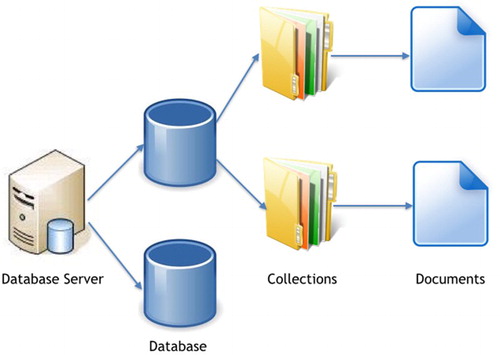
Figure 3 depicts the objects included in MongoDB and their relationships. MongoDB can host many databases on one server and each database houses a number of collections. Every collection stores any number of documents that are grouped by a set of key-value pairs in BSON format which is a binary-encoded serialization of JSON documents.

Figure 3. Components of the MongoDB database.

When storing tornado-related datasets, MongoDB offers a great deal of flexibility because it can store a wide variety of data types modeled in JSON format. In the FunnelCloud system, the database is designed to store spatial rasters of NARR variables and NEXRAD-based reflectivity fields, a time series of statistics generated from the NARR data, and geographical point datasets of NAXRAD radar station and tornado touchdown locations. The raster data are modeled using JSON arrays, and geographical point data are modeled using JSON key-value pairs. The schema for the FunnelCloud system is shown in Figure 4. The data warehouse is divided into three primary document databases that include documents containing the NARR grids, documents containing tornado touchdown data, and a database that contains the NEXRAD data. Each database consists of a number of collections and each collection contains documents modeled in JSON format. Figure 4 shows the layout of each document in detail including the field names. The symbol [ ] indicates that a particular data field is an array. The data dictionary which depicts detailed data types and descriptions for each document in the schema is shown in Table 2. The database also includes a file system layer that can be used for storing documents that exceed 16 MB in size such as images, audio files and video files. It is possible to store these files in a server file system, however, the GridFS system provides a number of advantages. For example, storing files in the database makes it easy to back up the files. Also, GridFS splits files into chunks and stores them separately, therefore, when querying a certain range of files, only those chunks will need to be brought into memory rather than the whole file. This saves memory when dealing with large files. Finally, when adding more files into GridFS system, the database can be distributed across different servers without increasing too much operational complexity.

Figure 4. FunnelCloud database schema.

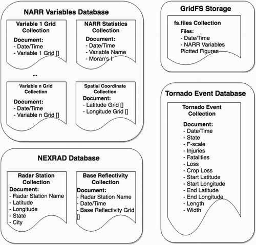
Table 2. Data dictionary for FunnelCloud system.

Field name	Data type	Description
NARR variable grid document
Data/Time	ISO 8601 Timestamp(UTC)	Timestamp of the NARR variable grid
NARR variable grid	Array	Grid for NARR variable (a grid exists for each variable at each time stamp)
Spatial coordinate document
Latitude grid	Array	Array of latitude coordinates that correspond directly to all NARR variables grids
Longitude grid	Array	Array of longitude coordinates that correspond directly to all NARR variables grids
NARRStatistics document
Date/Time	ISO 8601 Timestamp(UTC)	Timestamp of the NARR variable statistic
Variable name	String	NARR variable name
Moran's I	Double	Autocorrelation of NARR variable
Tornado event document
Date/Time	ISO 8601 Timestamp(UTC)	Timestamp of the tornado event
State	String	State of the tornado event
F-scale	Integer	F-scale of the tornado event
Injuries	Integer	Injuries caused by tornado event
Fatalities	Integer	Fatalities caused by tornado event
Loss	Integer	Estimated property loss
Crop Loss	Integer	Estimated crop loss
Start Latitude	Double	Starting latitude of tornado in decimal degrees
Start Longitude	Double	Starting longitude of tornado in decimal degrees
End Latitude	Double	Ending latitude of tornado in decimal degrees
End Longitude	Double	Ending longitude of tornado in decimal degrees
Length	Double	Tornado length in miles
Width	Double	Tornado width in yards
Radar station document
Radar Station Name	String	Radar station code
Latitude	Double	Latitude of radar station in decimal degrees
Longitude	Double	Longitude of radar station in decimal degrees
State	String	State of radar station
City	String	City of radar station
Base reflectivity document
Radar station name	String	Radar station code
Date/Time	ISO 8601 Timestamp(UTC)	Time stamp of radar image
Base reflectivity grid	Array	NEXRAD base reflectivity array

The NARR Variables database contains a set of collections including grids for each NARR variable, grids for geographic coordinates, and statistical data for each NARR variable. The NARR latitude and longitude grids assign each grid cell a set of geographic coordinates for all of the NARR variables. They are stored in a separate collection because the latitude and longitude values for each grid cell are static in nature. This standalone spatial coordinate collection saves storage resources because only the variable grids need to be stored for each time step. The NARR statistics collection contains documents for each variable where each document contains the spatial autocorrelation for a particular variable and time stamp. The variables, latitude, and longitude grids are stored as static numeric arrays. The NARR statistics documents are stored as time series. When storing time series data, it is a need to design an appropriate data schema, which depends on the data granularity and query scenarios. The time step of the time series data in NARR statistics collection are in 3 hours, and the primary method to query these data are based on a range of date. Therefore, all of the NARR statistics data are stored in one collection, and documents in collection contains data per daily. In this way, it is efficient to query relevant documents within one collection. All variables and NARR statistics collections are indexed on Date/Time. For example, the following shows an NARR variable document in JSON format for CAPE on 1 January 2015:

{

"Date/Time": "2015-01-01",

"CAPE Grid": [[…],[…], … ,[…]]

}

The Tornado Event Database includes a collection containing information about tornado events. Each tornado event is stored in its own document. Each document includes variables of Date/Time, state, F-scale, how many injuries and fatalities, how much property loss and crop loss, start latitude and longitude, end latitude and longitude, tornado length and tornado width. This tornado record collection is indexed on Date/Time.

The NEXRAD database contains two collections. The first contains metadata about radar stations including the radar station's name, latitude and longitude, and the radar stations state and city. The second collection stores the base reflectivity grids of each radar station. It contains the radar station name, Date/Time and base reflectivity grids that decoded from the original files of AWS services. Both of the two collections are indexed by radar station name and Date/Time since most of the data request from user interface and analysis layer are queried by radar station name and a range of Date/Time.

In the FunnelCloud data warehouse, the GridFS file system is used to store image files that are too large to be stored as BSON documents in normal MongoDB collections. These images stored into GridFS can be read easily, and then be used into user interface for visualization. For example, in our FunnelCloud system, the plotted figures of each NARR variable at each timestamp is stored into the file system. Once the web service requests these image files, the figures will be queried from the GridFS and loaded into web pages. The detailed process will be discussed in the web service and user interface section.

3.3. Extraction, transformation, and loading

ETL is a data warehousing process where data are extracted from different external sources, transformed into a destination format, and loaded into a data warehouse or data repository. A number of ETL processes are run on a periodic basis to load the source data into the FunnelCloud data warehouse. The ETL workflows presented in this section are depicted such that the source data are represented by the boxes on the left, intermediate processing steps are included in the subsequent boxes, and the database system is on the right. The ETL processes were developed in the Python programming language.

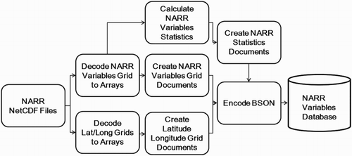
The ETL workflow for the NARR data is presented in Figure 5. The NARR data are available in NetCDF format which is a data format widely used by the geosciences community to manipulate array-oriented scientific data. The netCDF4-python API is used to decode each variable array, latitude array, and longitude array from NetCDF file. These arrays are then used to create JSON documents to represent each array. The JSON documents are then converted to BSON format and inserted into the NARR Variables Database. After that, the Moran's I for each variable in each time stamp is calculated. Moran's I is a measure of spatial autocorrelation that describes the correlation of a variable with itself through space. A negative Moran's I value means that similar values are not grouped, a positive value means similar values occur near one another, and zero indicates a random pattern (Moran 1950). Moran's I is calculated as follows:(1) where n is the number of spatial units, x is the meteorological variable, is the mean of x, is the weight between observation i and j, and is the sum of all 's: The Moran's I value is calculated as part of the ETL workflow because calculating it on the client side would be too computationally intensive. The NARR statistics documents include the Date/Time, the variable's name, and the Moran's I value. These documents are encoded to BSON and inserted into the NARR Variables Database.

Figure 5. ETL workflow for processing NARR data.

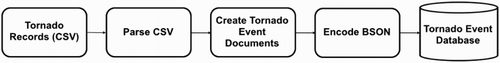
The tornado event data are available from NOAA's SPC in csv format. The ETL workflow for the tornado event data is presented in Figure 6. It first parses each csv file then encodes the event information for each tornado into a single JSON document. These documents are then serialized into BSON documents for loading into the Tornado Event Database in MongoDB.

Figure 6. ETL workflow for processing tornado record data.

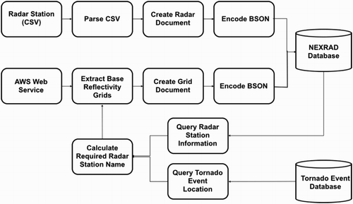
The ETL workflow for processing NEXRAD data is shown in Figure 7. The radar station information is available in csv format and base reflectivity data are available from Amazon's Web Service. The Boto python module is used to establish the AWS connection and then the interested base reflectivity grid data can be downloaded into local file. The ETL process parses the csv file and creates a document, then encodes it to BSON and stores it to the NEXRAD Database. After the radar station data is loaded into database, the base reflectivity grids are extracted. Base reflectivity grids for a given time step are only stored if a tornado occurred during that period. To accomplish this, Tornado Event Database is queried to determine the location of tornado events. Given this location, the closest NEXRAD station is found. Then the corresponding NEXRAD-based reflectivity data are downloaded from the AWS web service. These data are then converted to a JSON array, serialized into BSON format and loaded into the NEXRAD Database.

Figure 7. ETL workflow for processing radar data.

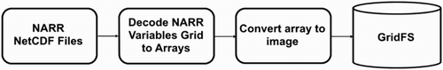
The workflow for loading NARR images into the GridFS file system is shown in Figure 8. In this step, the NARR NetCDF files are decoded and converted to arrays. Each array is then converted into an image. The resulting image files are then stored in GridFS. One image file represents one NARR variable at one time step. Given the large number of variables available at each time step, this results in thousands of images.

Figure 8. ETL workflow for processing NARR image files.

3.4. Spatio-temporal clustering

The FunnelCloud system uses a spatio-temporal clustering method to find tornado events that occur close in space and time. In particular, the ST-DBSCAN is used (Birant and Kut 2007). The ST-DBSCAN requires four parameters , , MinPts and . represents the distance between two points in space to be considered spatial neighbors, represents the distance of temporal attributes. MinPts is a density measurement that means a cluster must contain objects more than MinPts. The last parameter is used to prevent the discovery of combined clusters which means an object belongs to more than one cluster. In this method, each object is scanned and classified into three types including core objects, border objects and noise objects. If an object p is directly density-reachable from another object q that means the object p is within the neighborhood distances and of q, and q is a core object. If an object p is density-reachable from another object q, that means there is a chain between p and q that in the chain, each object is directly density-reachable from another. Thus, a border object represents an object that is not a core object but is density-reachable from another core object. A noise object is not density-reachable of any core objects. The algorithm then merges the core and border objects that are density reachable into one cluster. In the FunnelCloud system, the inputs to the ST-DBSCAN algorithm are the location and time stamp of the tornado events from the chosen date range. And the spatial threshold is set to 0.5 degrees which converts to about 30 miles, and the temporal threshold Eps2 is set to 24 hours. The MintPts threshold is set to ln(n) where n means the total tornado events. This threshold calculation method is recommended by Birant and Kut (2007) .

Figure 9 shows an example tornado dataset. Each sub figure represents a time step which ranges from 23 June to 26 June 2015. And the red lines in the map represent start location and end location of the tornado touchdown. Using this data combined with the ST-DBSCAN algorithm, a set of spatio-temporal tornado clusters can be generated. Each cluster will consist of a set of tornadoes that occur in close proximity of space and time. For example, the data in Figure 9 can generate four clusters, shown in Table 3. The ST-DBSCAN algorithm is also implemented using the Python programming language.

Figure 9. Example of spatio-temporal tornado dataset.

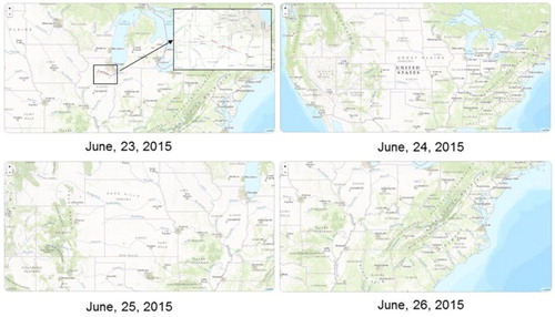
Table 3. Cluster result of data in Figure 9.

Longitude	Latitude	Time stamp	Cluster Result
−89.1334	41.5536	2015-6-23 T00:19:00	Cluster1
−89.107	41.5454	2015-6-23 T00:19:00	Cluster1
−89.1334	41.5454	2015-6-23 T00:19:00	Cluster1
−88.8719	41.4701	2015-6-23 T00:50:00	Cluster1
−88.762	41.4407	2015-6-23 T00:50:00	Cluster1
−83.7432	43.2542	2015-6-23 T01:00:00	Cluster2
−83.52	43.25	2015-6-23 T01:00:00	Cluster2
−83.52	43.2542	2015-6-23 T01:00:00	Cluster2
−83.7432	43.2542	2015-6-23 T01:00:00	Cluster2
−83.1308	43.5031	2015-6-23 T01:07:00	Cluster2
−81.8507	41.1647	2015-6-23 T02:08:00	Cluster3
−80.8507	41.1785	2015-6-23 T02:08:00	Cluster3
−82.8224	42.9567	2015-6-23 T02:55:00	Cluster3
−82.8099	42.9561	2015-6-23 T02:55:00	Cluster3
−71.3335	42.065	2015-6-23 T20:35:00	Cluster4
−71.3245	42.067	2015-6-23 T20:35:00	Cluster4
−71.3245	42.065	2015-6-23 T20:35:00	Cluster4
−71.3335	42.067	2015-6-23 T20:35:00	Cluster4

3.5. Web service architecture

The web services architecture of the FunnelCloud system is presented in Figure 10. The Python programming language was also used for implementing the web services where the pyMongo module was used to query data from the MongoDB data warehouse, and Flask, which is a lightweight python web framework, was used to provide RESTful web services. In the Representational State Transfer (REST) web service protocol, data are considered to be a resource that can be accessed using Uniform Resource Identifiers (URIs). In the FunnelCloud system, clients have access to various data by using an http request where a query string is coded in the URL. The query string includes parameters that conditionally request data based on the value of a variable. In the FunnelCloud system, the web services require a dataset name and a date range. The request is formatted as a URL string such as http://serverIP:serverPort/Dataset/FromDate/ToDate. The Dataset string is encoded to represent different dataset names, such as tornado or radar station. The FromDate and ToDate strings are encoded to YYYY-MM-DD date format, such as 2015-01-01. Then a JSON document that contains the corresponding variables value will be returned. This modular processing technique allows clients to request data from various web services simultaneously.

Figure 10. Overview of web service architecture.

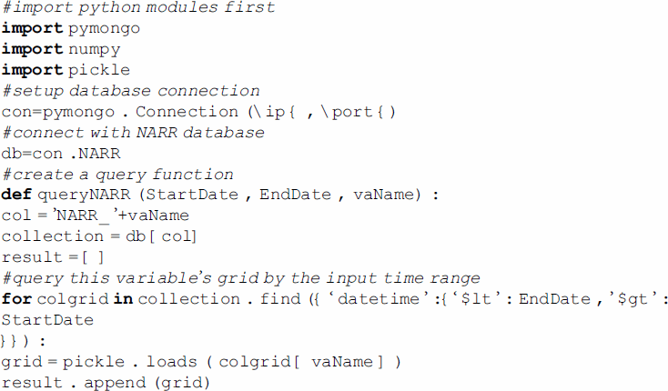
In the FunnelCloud system, a number of MongoDB queries have been developed. For example, one of the most useful queries is to query the NARR variable grid data. It can be used to calculate descriptive statistics for NARR variables of interest. An example of this query is shown below. This example uses the pyMongo module to create a query function that requires a variable name and a date range. Then the function returns a collection of grids for the variable of interest. In this example, first the connection to MongoDB is set up by using the MongoDB database server's IP address and port number. Then, the gridded data are returned in BSON format and decoded into a JSON document. Each grid is then appended into the result array. It is possible to develop more complex queries using this framework. For example, the query that returns the NEXRAD-based reflectivity data, uses the location and date range of the tornado event to return the relevant set of radar images. An example of the result of this query is shown in the next section.

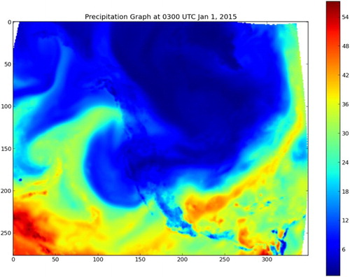
Since the web service provides a RESTful interface, the returned result data are easily consumed by visualization tools. One example graph is shown in Figure 11. It utilizes the above query function combined with the matplotlib module in Python to plot precipitation data for 1 January 2015.

Figure 11. Precipitation graph at 0300 UTC 1 January 2015.

3.6. User interface and visualization

The FunnelCloud web interface consists of several components, including an interactive map, a dynamic timeline, a spatial statistics table, a map-based radar data visualization, an NARR statistical graph and an NARR variables data visualization. The detailed web client workflow is shown in Figure 12.

Figure 12. Web client workflow of the FunnelCloud system.

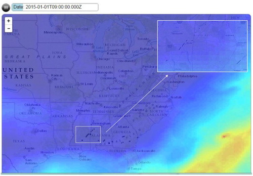
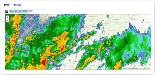
The first step in the user interface workflow requires the user to choose a date range using the interactive timeline view in the bottom of the web page, as shown in Figure 13. The timeline view is implemented by d3.js (https://d3js.org/), which is a JavaScript library for web-based data visualization. The timeline date range in the prototype system is from 1 January 2015 to 31 December 2015. The blue color on the time line indicates that a tornado event occurred during that time period. Once a time range is chosen, individual tornado event trajectories are represented by red lines and tornado clusters are represented by blue rectangles on the map view. The map view is implemented using the Leaflet web mapping API (http://leafletjs.com/), which is a JavaScript library for interactive web mapping. The analysis view presents the number of spatio-temporal clusters along with a list of NARR variables. Using this interface, the user can choose a particular variable and a number of ways to analyze the data. If the NARR variable visualization is selected, a new window is spawned which includes a play button, a play time bar and a map view. This view shows an animation of the selected NARR variable. Figure 14 shows an example animation of precipitable water from 1 January to 4 January 2015. The figure shows a screenshot taken at 9 AM on 1 January 2015. The black lines on the map represent tornado events that occurred during this time period. And the shading on the map shows precipitable water values from red (high) to blue (low).

Figure 13. User interface of the FunnelCloud system.

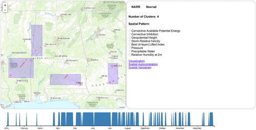
Figure 14. Visualization showing NARR variables and tornado locations.

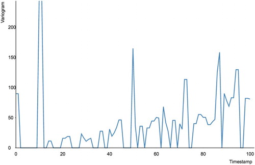
If the user chooses to see the spatial autocorrelation or spatial variogram on the NARR data analysis page, a new window will show a line graph of the statistical data over time. An example of this graph is shown in Figure 15.

Figure 15. Example of a spatial variogram for CAPE from 24 March 2015 to 19 April 2015.

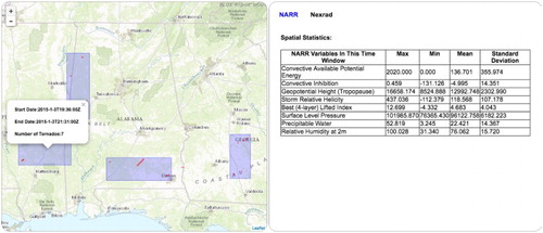
If a red line on the map view is clicked by the user, a pop up window will display detailed information for the tornado event including the date, time, state, and F-scale of this particular tornado. If a spatio-temporal cluster (blue rectangle) is clicked on the interactive map, a pop-up window will display the start date, start time, end date, end time, and the number of tornado events in the cluster. The analysis tab will then include an animation of the relevant NEXRAD-based reflectivity data for this spatio-temporal cluster. This visualization is depicted in Figure 16.

Figure 16. NEXRAD loop for a selected spatio-temporal cluster.

If the user clicks the NARR tab after choosing a spatio-temporal cluster, a descriptive table will show the descriptive statistics of the relevant NARR variables (Figure 17). In this table, rows represent the NARR variables, and columns represent the descriptive statistic including the maximum, minimum, mean, and standard deviation of the NARR variable. The statistical values are calculated from the NARR grid cells that are near the location of the tornado cluster.

Figure 17. Descriptive statistics table for NARR variables.

3.7. FunnelCloud performance

An experiment was designed to test the performance of the FunnelCloud system in generating spatio-temporal tornado clusters for varying date ranges. The experiment was performed on a Dell Optiplex 990 desktop computer with 8GB of RAM and a 3.40 GHZ processor using the Google Chrome web browser. The date range of the query was set to 1, 10, 30, 180, and 365 days. Because most of the tornadoes in the year 2015 occurred during the spring and summer months, the month of May was chosen for the date range of 1, 10, and 30 days and May to July was chosen for the 180 days date range.

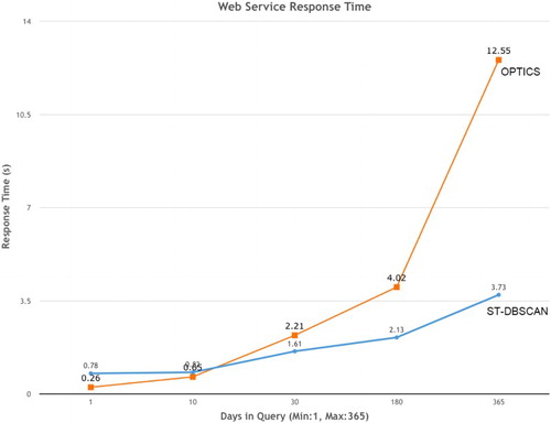
To test the performance of the ST-DBSCAN algorithm, we have compared it with OPTICS (Ordering Points To Identify the Clustering Structure), which is another well-known density-based clustering algorithm for spatial datasets. Since OPTICS does not deal with the temporal dimension, the method used in this experiment only takes the spatial dimension of tornado events as input. To test the performance of the algorithm, both ST-DBSCAN and OPTICS were incorporated in the web service and the time to complete the query was measured with a varying number of days. The spatial dimension threshold for OPTICS was set to 30 miles, and the minimum points in a cluster was set to ln(n) as the same as ST-DBSCAN. The result of the performance comparison is shown in Figure 18. Here it is evident that the web service response time when using ST-DBSCAN grows slowly as the date range increases as compared with the web service using OPTICS. When the number of days is set to 365, the response time of OPTICS is about 13 seconds, while the response time of ST-DBSCAN is only about 4 seconds. This is because the time complexity of ST-DBSCAN is O(n * log n), where n is the number of objects in the dataset. In our experiment, n means the total number of tornado events that occurred during the chosen date range. But the time complexity of OPTICS is O(). Therefore, for a dataset with a large number of points, ST-DBSCAN performs better than OPTICS.

Figure 18. Comparison of web service response time between ST-DBSCAN and OPTICS.

4. Use case: analyzing the thermodynamic and kinematic parameters, and the NEXRAD images, corresponding to tornado clusters

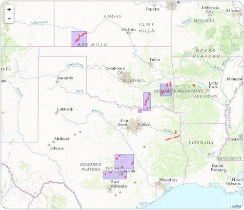
Forty tornadoes were produced on 25 May 2015 (UTC). Most of these were located in the south-central United States and one isolated tornado occurred in Florida, shown in Figure 19. Fifty-eight percent of these tornadoes were organized into five clusters of more than one tornado: Cluster A included 7 tornadoes produced in southwest Kansas between 0137 and 0420 UTC; Cluster B included 3 tornadoes produced in central Texas between 1633 and 2024 UTC; Cluster C included 5 tornadoes produced in central Texas between 1741 and 1955 UTC; Cluster D included 4 tornadoes in northern Texas and southern Oklahoma between 1842 and 2006 UTC; Cluster E included 4 tornadoes in eastern Oklahoma between 2052 and 2148 UTC.

Figure 19. Individual tornadoes (red dots and lines) and tornado clusters (transparent blue polygons) that occurred on 25 May 2015.

4.1. Thermodynamic and kinematic indices

NARR provides multiple thermodynamic (i.e. those that describe atmospheric instability) and kinematic (i.e. those that describe atmospheric motion) parameters that are useful when describing and analyzing severe weather events. CAPE and the lifted index (LI) represent atmospheric stability. Positive values of CAPE and negative values of LI denote unstable conditions that are favorable for thunderstorms and tornadoes. Convective inhibition (CIN) represents the negative buoyancy that must be overcome for thunderstorm initiation, and therefore tornado production. Low-to-moderate, negative values of CIN are more favorable for tornadoes than larger negative values because environments with large CIN tend to suppress thunderstorm initiation (Davies 2004). Storm relative helicity (SRH) represents the potential for cyclonic updraft rotation. Larger, positive values denote an increased chance for supercellular thunderstorms and tornadoes. A review of these parameters and their interpretation is provided by Thompson (2016) .

Table 4 presents statistical descriptions of the thermodynamic and kinematic environments associated with the tornado clusters using the above-mentioned parameters. These statistics were taken from the NARR variables statistical tables in the FunnelCloud system. The mean values of the CAPE and LI parameters show that the environments in which these tornadoes occurred were unstable. Furthermore, the max values of CAPE associated with three of the clusters that were and the min values of LI associated with all of the clusters that were show that at least some areas within the cluster polygons were extremely unstable and favorable for severe thunderstorms and tornadoes. The moderate mean values of CIN () illustrate that there was not much negative buoyancy to overcome, and that thunderstorm formation was favored, especially when considering the instability. Lastly, the mean and max values of SRH were for all clusters except cluster A. These values indicate that supercell thunderstorm formation is likely in these environments than in those with values in excess of . The mean and max values of SRH associated with cluster A () were more favorable for supercell formation.

Table 4. Descriptive statistics summarizing the thermodynamic and kinematic environments corresponding to the tornado clusters on 25 May 2015.

	CAPE ()
Cluster	Max	Min	Mean	SD
A	2050	560	1369	387
B	4530	0	897	1304
C	4220	1170	2919	728
D	2090	0	410	534
E	5260	140	2655	1240
	3630	374	1650	839
	LI (K)
Cluster	Max	Min	Mean	SD
A	−3	−7	−5	1
B	9	−9	1	6
C	−3	−11	−8	2
D	2	−9	−2	3
E	−1	−13	−7	3
	1	−10	−4	3
	CIN ()
Cluster	Max	Min	Mean	SD
A	−2	−93	−46	23
B	0	−139	−28	40
C	0	−91	−24	23
D	0	−89	−33	26
E	0	−65	−11	15
	0	−95	−28	25
	SRH ()
Cluster	Max	Min	Mean	SD
A	420	156	301	70
B	239	38	119	51
C	223	15	106	54
D	77	23	44	1
E	232	−9	68	49
	238	45	128	47

Note: CAPE, convective available potential energy; LI, best (4-layer) lifted index; CIN, convective inhibition; SRH, storm relative helicity; Max, maximum value; Min, minimum value; Mean, mean value; SD, standard deviation. of cluster values.

4.2. NEXRAD images

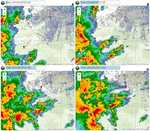
NEXRAD images corresponding to the tornadoes in the clusters are shown in Figures 20–24. The series illustrate well the ability of FunnelCloud to display tornado and parent storm locations. Figure 20, for example, shows that the seven tornadoes in cluster A were produced by a cell with supercellular structure (panels E–G) that began as two cells (panels A and B). The tornadoes in the other four clusters were produced by a mesoscale convective system, which is a cluster of thunderstorms, that moved across the region later in the afternoon.

Figure 20. NEXRAD base reflectivity corresponding to the seven tornadoes in cluster A. Panel A–G show the base reflectivity at 0138 UTC, 0146 UTC, 0206 UTC, 0220 UTC, 0248 UTC, 0327 UTC and 0419 UTC and corresponds to the EF1, EF0, EF0, EF0, EF1, EF2 and EF1 tornadoes that began at 0137 UTC, 0147 UTC, 0206 UTC, 0220 UTC, 0247 UTC, 0326 UTC and 0420 UTC, respectively. The Ts in the figure denote the start locations of the tornadoes.

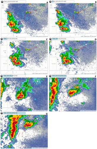
Figure 21. NEXRAD base reflectivity corresponding to the seven tornadoes in cluster B. Panel A–C show the base reflectivity at 1634 UTC, 1703 UTC, 2022 UTC and corresponds to the EF1, EF0 and EF1 tornadoes that began at 1633 UTC, 1704 UTC and 2024 UTC, respectively. The Ts denote the start locations of the tornadoes.

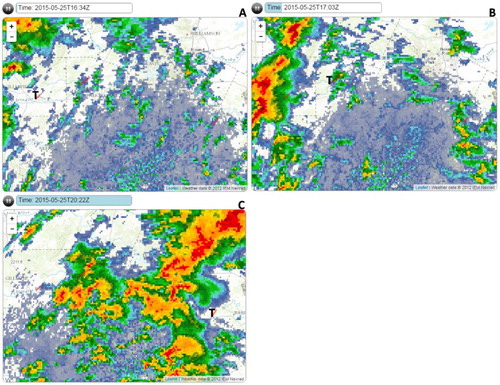
Figure 22. NEXRAD-based reflectivity corresponding to the seven tornadoes in cluster C. Panel A shows the base reflectivity at 1743 UTC and corresponds to the two EF1 tornadoes that began at 1741 and 1742 UTC. Panel B–D show base reflectivity at 1805 UTC, 1845 UTC and 1953 UTC and corresponds to the EF1, EF1 and EF2 tornadoes that began at 1806 UTC, 1845 UTC and 1955 UTC, respectively. The Ts denote the start locations of the tornadoes.

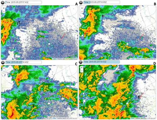
Figure 23. NEXRAD-based reflectivity corresponding to the seven tornadoes in cluster D. Panel A–D show the base reflectivity at 1843 UTC, 1929 UTC, 1942 UTC and 2005 UTC and corresponds to the EF3, EF2, EF0 and EF1 tornadoes that began at 1842 UTC, 1929 UTC, 1941 UTC and 2006 UTC, respectively. The Ts denote the start locations of the tornadoes.

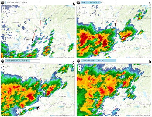
Figure 24. NEXRAD-based reflectivity corresponding to the seven tornadoes in cluster E. Panel A–D show the base reflectivity at 2053 UTC, 2116 UTC, 2134 UTC and 2147 UTC and corresponds to the EF2, EF1, EF1, EF2 tornadoes that began at 2052 UTC, 2117 UTC, 2134 UTC and 2148 UTC, respectively. The Ts denote the start locations of the tornadoes.

4.3. Other potential use cases

This use case illustrates the capability of FunnelCloud by describing and analyzing the thermodynamic and kinematic environments, and the NEXRAD images, associated with the tornadoes that occurred on 25 May 2015, but the system is capable of other applications. For instance, only one day was examined here, but longer periods of time could be analyzed to extract generalizations, develop climatologies, and detect temporal trends in tornado favorable environments. These capabilities are valuable to current efforts directed toward detecting and analyzing trends in tornado frequencies and tornado-favorable environmental parameters, as they relate to climate change (e.g. Elsner, Elsner, and Jagger 2015; Tippett et al. 2015).

The assimilation of NEXRAD and tornado data could be used to inspect information and even estimate missing information in the tornado record, such as start and end coordinates and times, path lengths, and path widths. The tornado shown in Figure 20(C), for example, does not coincide in space and time with the convective cell to its southwest that likely produced it. Other examples of spatio-temporal separation seen here between the tornado start coordinates and times and the locations of candidate parent storm cells include: Figure 21(A) and 21(C); Figure 22(D); Figure 23(A)–(D) ; Figure 24(A)–(D). Identification of such instances, along with additional analysis, could help improve the accuracy of the start coordinates and/or times of the impacted tornadoes.

5. Future works and conclusions

This paper presents a FunnelCloud system that integrates different sources of tornado-related datasets for tornado events exploration and analysis. The database design of the FunnelCloud system is implemented by a flexible and scalable document database, MongoDB. Also, a set of ETL workflows are developed to show the steps of how to insert data into the document database. Furthermore, ST-DBSCAN which is a spatio-temporal clustering method is implemented on clustering tornado event dataset based on both spatial and temporal similarities. And a set of RESTful web services provide access to the integrated dataset and a map-based user interface provides an interactive visualization and exploratory of tornado event analysis. The utility of the FunnelCloud system was demonstrated in a use case that analyze the tornado cluster's thermodynamic and kinematic parameters and radar images. In general, the FunnelCloud system offers a great deal of flexibility that allows scientist to create custom tornado analysis and an extreme amount of scalability that allows the system be scaled out into multiple nodes.

There are a number of future enhancements in which this research can be extended. First, the prototype system presented in this paper consists of only one year data. This dataset only requires one MongoDB node. We would like to extend the FunnelCloud system to include a longer duration tornado events data, and scale the database to multiple nodes. Second, we would also like to develop a storm tracking method to identify and track the movement of supercells associated with tornado touchdowns. Another potential future application would be to apply sequential pattern mining algorithms to predict tornado events based on sequences found in the time series of the NARR variables. Finally, we would like to develop additional user interfaces to facilitate a deeper analysis of tornado events. This can include the combined visualization of NEXRAD and NARR data as well as the visualization of the results of storm/tornado tracking algorithms more.

Disclosure statement

No potential conflict of interest was reported by the authors.

ORCID

Todd W. Moore http://orcid.org/0000-0001-8600-5555

References

- Aji, Ablimit, and Fusheng Wang. 2012. “High Performance Spatial Query Processing for Large Scale Scientific Data.” In Proceedings of the on SIGMOD/PODS 2012 PhD Symposium, Scottsdale, AZ, USA, 9–14. New York, NY: ACM Press.
- Aji, Ablimit, Fusheng Wang, and Joel H. Saltz. 2012. “Towards Building a High Performance Spatial Query System for Large Scale Medical Imaging Data.” In Proceedings of the 20th International Conference on Advances in Geographic Information Systems, Redondo Beach, CA, USA, 309–318. New York, NY: ACM.
- Armbrust, Michael, Armando Fox, Rean Grith, Anthony D. Joseph, Randy H. Katz, Andrew Konwinski, and Gunho Lee, et al. 2009. “Above the Clouds: A Berkeley View of Cloud Computing.” Tech. Rep. UCB/EECS-2009-28, EECS Department, U.C. Berkeley, February 2009.
- AWS. 2016. “Next Generation Weather Radar (NEXRAD) on Amazon Web Service (AWS).” https://aws.amazon.com/noaa-big-data/nexrad/.
- Barros, V. R., C. B. Field, D. J. Dokke, M. D. Mastrandrea, K. J. Mach, T. E. Bilir, and M. Chatterjee, et al. 2014. “Climate Change 2014: Impacts, Adaptation, and Vulnerability. Part B: Regional Aspects. Contribution of Working Group II to the Fifth Assessment Report of the Intergovernmental Panel on Climate Change.”
- Birant, Derya, and Alp Kut. 2006. “An Algorithm to Discover Spatial-Temporal Distributions of Physical Seawater Characteristics and a Case Study in Turkish Seas.” Journal of Marine Science and Technology 11 (3): 183–192. doi: 10.1007/s00773-005-0213-2
- Birant, Derya, and Alp Kut. 2007. “ST-DBSCAN: An Algorithm for Clustering Spatial-Temporal Data.” Data & Knowledge Engineering 60 (1): 208–221. doi: 10.1016/j.datak.2006.01.013
- Brezany, Peter, Yan Zhang, Ivan Janciak, Peng Chen, and Sicen Ye. 2011. “An Elastic OLAP Cloud Platform.” In 2011 IEEE Ninth International Conference on Dependable, Autonomic and Secure Computing (DASC), 356–363. IEEE.
- Camp, J., M. Roberts, C. MacLachlan, E. Wallace, L. Hermanson, A. Brookshaw, A. Arribas, and A. A. Scaife. 2015. “Seasonal Forecasting of Tropical Storms using the Met Office GloSea5 Seasonal Forecast System.” Quarterly Journal of the Royal Meteorological Society 141 (691): 2206–2219. http://dx.doi.org/10.1002/qj.2516. doi: 10.1002/qj.2516
- Cao, Yu, Chun Chen, Fei Guo, Dawei Jiang, Yuting Lin, Beng Chin Ooi, Hoang Tam Vo, Sai Wu, and Quanqing Xu. 2011. “Es 2: A Cloud Data Storage System for Supporting Both Oltp and Olap.” In 2011 IEEE 27th International Conference on Data Engineering, Hannover, 291–302. IEEE.
- Coletti, Alex, Peter D. Howe, Brent Yarnal, and Nathan J. Wood. 2013. “A Support System for Assessing Local Vulnerability to Weather and Climate.” Natural Hazards 65: 999–1008. doi: 10.1007/s11069-012-0366-3
- Cox, A. T., J. A. Greenwood, V. J. Cardone, and V. R. Swail. 1995. “An Interactive Objective Kinematic Analysis System.” International Workshop on Wave Hindcasting and Forecasting. October.
- Crockford, Douglas. 2006. “The Application/json Media Type for Javascript Object Notation (json).” https://tools.ietf.org/html/rfc4627.
- Davies, Jonathan M. 2004. “Estimations of CIN and LFC Associated with Tornadic and Nontornadic Supercells.” Weather and Forecasting 19 (4): 714–726. doi: 10.1175/1520-0434(2004)019<0714:EOCALA>2.0.CO;2
- Dyer, Tristan, and John Baugh. 2016. “SMT: An Interface for Localized Storm Surge Modeling.” Advances in Engineering Software 92: 27–39. doi: 10.1016/j.advengsoft.2015.10.003
- Elsner, James B., Svetoslava C. Elsner, and Thomas H. Jagger. 2015. “The Increasing Efficiency of Tornado Days in the United States.” Climate Dynamics 45 (3-4): 651–659. doi: 10.1007/s00382-014-2277-3
- Grazulis, Thomas P. 1990. Significant Tornadoes, 1880–1989: A Chronology of Events. Vol. 2. St. Johnsburg, VT: Environmental Films.
- Han, Youn-Hee, Doo-Soon Park, Weijia Jia, and Sang-Soo Yeo. 2013. Ubiquitous Information Technologies and Applications. Lecture Notes in Electrical Engineering Vol. 214, Netherlands.
- Heard, J. R. 2011. Geoanalytics. Technical report. Technical Report TR-11-03, Renaissance Computing Institute.
- Hoffman, Forrest M, William W. Hargrove Jr, David J. Erickson III, and Robert J. Oglesby. 2005. “Using Clustered Climate Regimes to Analyze and Compare Predictions from Fully Coupled General Circulation Models.” Earth Interactions 9 (10): 1–27. doi: 10.1175/EI110.1
- Jansen, Wayne A. 2011. “Cloud Hooks: Security and Privacy Issues in Cloud Computing.” In 2011 44th Hawaii International Conference on System Sciences (HICSS), 1–10. IEEE.
- Kalnay, Eugenia. 2003. Atmospheric Modeling, Data Assimilation and Predictability. New York: Cambridge University Press.
- Lakshmanan, Valliappa. 2001. “A Hierarchical, Multiscale Texture Segmentation Algorithm for Real-World Scenes.” Ph.D. thesis. The University of Oklahoma.
- Lakshmanan, Valliappa, and Travis Smith. 2009. “Data Mining Storm Attributes from Spatial Grids.” Journal of Atmospheric and Oceanic Technology 26 (11): 2353–2365. doi: 10.1175/2009JTECHA1257.1
- Maidment, D. 2006. “Hydrologic Information Systems.” Austin, USA. http://adsabs.harvard.edu/abs/2006AGUFMIN21A1209M.
- McGuire, Michael P., Martin C. Roberge, and Jie Lian. 2016. “Channeling the Water Data Deluge: A System for Flexible Integration and Analysis of Hydrologic Data.” International Journal of Digital Earth 9 (3): 272–299. doi: 10.1080/17538947.2015.1031715
- Mell, Peter, and Tim Grance. 2011. “The NIST Definition of Cloud Computing.” US Nat'l Inst. of Science and Technology, 2011.
- Mesinger, Fedor, Geoff DiMego, Eugenia Kalnay, and Kenneth Mitchell, et al. 2006. “North American Regional Reanalysis.” Bulletin of the American Meteorological Society 87 (3): 343–360. doi: 10.1175/BAMS-87-3-343
- Moran, Patrick A. P. 1950. “Notes on Continuous Stochastic Phenomena.” Biometrika 37 (1/2): 17–23. doi: 10.2307/2332142
- NEXRAD, NOAA National Weather Service (NWS) Radar Operations Center. 2016. “NOAA Next Generation Radar (NEXRAD) Level II Base Data.” http://www.ncdc.noaa.gov/nexradinv/map.jsp.
- OGC. 2016. “Open Geospatial Consortium, Inc (OGC) Web Services.” https://mesonet.agron.iastate.edu/ogc/.
- Powell, Mark D., Sam H. Houston, Luis R. Amat, and Nirva Morisseau-Leroy. 1998. “The HRD Real-Time Hurricane Wind Analysis System.” Journal of Wind Engineering and Industrial Aerodynamics 77–78: 53–64. doi: 10.1016/S0167-6105(98)00131-7
- SPC. 2016. “National Oceanic and Atmospheric Administration/National Climatic Data Centers (NOAA/NCDC) Storm Prediction Center (SPC).” http://www.spc.noaa.gov/gis/svrgis/.
- Steinhaeuser, Karsten, Auroop R. Ganguly, and Nitesh V. Chawla. 2012. “Multivariate and Multiscale Dependence in the Global Climate System Revealed Through Complex Networks.” Climate Dynamics 39 (3/4): 889–895. doi: 10.1007/s00382-011-1135-9
- Strauss, Cesar, Marcelo Barbio Rosa, and Stephan Stephany. 2013. “Spatio-Temporal Clustering and Density Estimation of Lightning Data for the Tracking of Convective Events.” Atmospheric Research 134: 87–99. doi: 10.1016/j.atmosres.2013.07.008
- Thompson, Rich. 2016. “Explanation Of SPC Severe Weather Parameters.” http://www.spc.noaa.gov/exper/mesoanalysis/help/begin.html
- Thusoo, Ashish, Joydeep Sen Sarma, Namit Jain, Zheng Shao, Prasad Chakka, Ning Zhang, Suresh Antony, Hao Liu, and Raghotham Murthy. 2010. “Hive-a Petabyte Scale Data Warehouse using Hadoop.” In 2010 IEEE 26th International Conference on Data Engineering (ICDE 2010), 996–1005. Long Beach, CA, USA. IEEE.
- Tippett, Michael K., John T. Allen, Vittorio A. Gensini, and Harold E. Brooks. 2015. “Climate and Hazardous Convective Weather.” Current Climate Change Reports 1 (2): 60–73. doi: 10.1007/s40641-015-0006-6
- Yang, Chaowei, Michael Goodchild, Qunying Huang, Doug Nebert, Robert Raskin, Yan Xu, Myra Bambacus, and Daniel Fay. 2011. “Spatial Cloud Computing: How can the Geospatial Sciences use and help Shape Cloud Computing?.” International Journal of Digital Earth 4 (4): 305–329. doi: 10.1080/17538947.2011.587547