Automatic sub-pixel co-registration of Landsat-8 Operational Land Imager and Sentinel-2A Multi-Spectral Instrument images using phase correlation and machine learning based mapping

ABSTRACT

This study investigates misregistration issues between Landsat-8/ Operational Land Imager and Sentinel-2A/ Multi-Spectral Instrument at 30 m resolution, and between multi-temporal Sentinel-2A images at 10 m resolution using a phase-correlation approach and multiple transformation functions. Co-registration of 45 Landsat-8 to Sentinel-2A pairs and 37 Sentinel-2A to Sentinel-2A pairs were analyzed. Phase correlation proved to be a robust approach that allowed us to identify hundreds and thousands of control points on images acquired more than 100 days apart. Overall, misregistration of up to 1.6 pixels at 30 m resolution between Landsat-8 and Sentinel-2A images, and 1.2 pixels and 2.8 pixels at 10 m resolution between multi-temporal Sentinel-2A images from the same and different orbits, respectively, were observed. The non-linear random forest regression used for constructing the mapping function showed best results in terms of root mean square error (RMSE), yielding an average RMSE error of 0.07 ± 0.02 pixels at 30 m resolution, and 0.09 ± 0.05 and 0.15 ± 0.06 pixels at 10 m resolution for the same and adjacent Sentinel-2A orbits, respectively, for multiple tiles and multiple conditions. A simpler 1st order polynomial function (affine transformation) yielded RMSE of 0.08 ± 0.02 pixels at 30 m resolution and 0.12 ± 0.06 (same Sentinel-2A orbits) and 0.20 ± 0.09 (adjacent orbits) pixels at 10 m resolution.

KEYWORDS:

• Sub-pixel co-registration
• phase correlation
• misregistration
• Landsat-8
• Sentinel-2
• machine learning
• random forest

1. Introduction

Many applications in climate change and environmental and agricultural monitoring rely heavily on the exploitation of multi-temporal satellite imagery. Multi-temporal satellite images can help to identify and analyze changes in land cover land use change (LCLUC) (Justice, Gutman, and Vadrevu 2015), to capture significant trends in land surface properties, for example, greenness (Ju and Masek 2016), or to discriminate specific crop types (Shelestov et al. 2017; Skakun et al. 2016), that cannot be identified with a single date image. In order to solve these problems more efficiently at high spatial resolutions (30 m), combined use of freely available Landsat-8 and Sentinel-2 images can offer high temporal frequency of about 1 image every 3–5 days globally.

Landsat-8 was launched in 2013 within the Landsat Program, a joint effort between the U.S. Geological Survey (USGS) and NASA (Roy et al. 2014). The Operational Land Imager (OLI) and Thermal Infrared Sensor (TIRS) instruments onboard the Landsat-8 satellite capture images of the Earth’s surface in 11 spectral bands of the electromagnetic spectrum at 30 m spatial resolution (15 m for panchromatic band and 100 m for thermal infrared). The swath of Landsat-8 scene is approximately 185 km, allowing global coverage of the Earth’s surface every 16 days. To refine image geolocation, the Landsat-8 processing uses ground control points automatically derived from the Global Land Survey (GLS) Landsat images (Gutman et al. 2013). The Sentinel-2A satellite was launched in 2015 within the European Copernicus program (Drusch et al. 2012). Sentinel-2A has a Multi-Spectral Instrument (MSI) that acquires images of the Earth’s surface in 13 spectral bands at 10 m, 20 m and 60 m spatial resolution. The swath of a Sentinel-2A scene is approximately 290 km, allowing global coverage of the Earth’s surface every 10 days. The launch of an identical Sentinel-2B satellite will further reduce revisit time to 5 days globally. Both Sentinel-2A/B satellites will use a Global Reference Image (GRI) derived from orthorectified Sentinel-2 cloud-free images to improve geolocation accuracy and repeatability to meet the requirements of multi-temporal registration of 3 m for 10 m bands (Dechoz et al. 2015). The GRI dataset is currently under development and is expected to be completed in 2018 (Storey et al. 2016).

Recent studies are focusing on the combined use of Landsat-8 and Sentinel-2A images to increase temporal coverage; however misregistration issues between Landsat-8 and Sentinel-2A have already been identified (Storey et al. 2016). It has been found that the OLI and MSI misregistration can exceed one 30-meter pixel and, therefore, it is recommended to exploit image registration approaches to further improve alignment between Landsat-8 and Sentinel-2A images (Storey et al. 2016). These approaches should be automatic and computationally efficient in order to perform alignment on a global basis, have sub-pixel accuracy and effectively deal with temporal changes, so these approaches can be further applied with GLS and GRI.

There have been many studies carried out to develop automatic satellite image registration methods (e.g. Gao, Masek, and Wolfe 2009; Le Moigne, Netanyahu, and Eastman 2011; Zitova and Flusser 2003). The general image-to-image registration workflow consists of automatic generation of control points (CPs) between the reference (or master) and sensed (or slave) images, building and evaluating a spatial transformation (mapping function) that aligns the reference and sensed images, and warping the sensed image with radiometric transformation. Area-based and feature-based approaches are used to automatically derive CPs. Area-based methods, also referred to as correlation-like or template matching, find correspondence between reference and sensed images through a similarity measure, for example cross-correlation (in spatial or frequency domain) or mutual information. These measures are usually applied on a sliding window basis to derive a dense set of CPs. Feature-based methods aim to find distinctive features on images, for example edges, contours, line intersections, closed boundary regions, and then match the derived features to find correspondences between reference and sensed images. The derived CPs are used to construct and evaluate a mapping function that maps points from the reference image to points in the sensed image. Examples of the mapping function include translation, affine transformation, high-order polynomials, radial basis functions (RBFs), and elastic registration. And finally, radiometric transformation (nearest neighbor, bilinear and splines) should be specified to warp the sensed image to the reference one.

The problem of Landsat-8/OLI and Sentinel-2A/MSI misregistration has already been addressed in several previous studies (Barazzetti, Cuca, and Previtali 2016; Yan et al. 2016). Yan et al. (2016) used a hierarchical feature-based matching approach to find CPs through construction of image pyramids at various spatial resolutions and an area-based matching approach to further refine and reject non-reliable CPs. Translation, affine transformation and second order polynomial functions were evaluated in the study for three pairs of Landsat-8 and Sentinel-2A images with affine transformation giving the best results in terms of root mean square error (RMSE) of 0.3 pixels at 10 m resolution. Barazzetti, Cuca, and Previtali (2016) utilized standard software packages to study misregistration between Landsat-8 and Sentinal-2A, and achieved RMSE of up to 1.2 pixels at 15 m spatial resolution.

In this paper, we explore a phase-correlation approach to automatically generate a dense grid of CPs when registering Landsat-8 to Sentinel-2A images, as well as multiple mapping functions including those based on machine learning approaches. We also address the issue of multi-temporal misregistration between Sentinel-2A images (for assessment of registration accuracy of multi-temporal Landsat-8 images, we refer readers to Storey, Choate, and Lee (2014)). Our analysis shows misregistration magnitudes of up to 3 pixels at 10 m resolution can be observed. This issue has not been reported in previous studies to our knowledge (except Sentinel-2 Data Quality Reports, see ESA (2016a), and reports delivered at the LCLUC Multi-Source Land Imaging (MuSLI) Science Team Meeting 2016, http://lcluc.umd.edu/meetings/2016-lcluc-spring-science-team-meeting-18-19-april-and-musli-science-team-meeting-20-21), and should be further addressed especially for users dealing with Sentinel-2A time-series at 10 m spatial resolution. As in Yan et al. (2016), we use near-infrared (NIR) bands from Landsat-8 (band 5, 0.85–0.88 um) and Sentinel-2A (band 08, 0.842 um) to find CPs on reference and sensed images, since the NIR provides a wide dynamic range of values for multiple land cover types and is less sensitive to atmospheric effects. Co-registration of Landsat-8 to Sentinel-2A was performed at 30 m spatial resolution while co-registration between Sentinel-2A images was undertaken at 10 m spatial resolution.

2. Data description

2.1. Landsat-8 and Sentinel-2A products description

We used a standard Landsat-8 Level-1 terrain corrected (L1 T) product distributed by USGS through the EarthExplorer system (Roy et al. 2014). The product is provided in the World-wide Reference System (WRS-2) of path and row coordinates. The size of the Landsat-8 scene is approximately 185 km × 180 km. The product is provided with the corresponding metafile to convert digital numbers (DNs) into the top-of-atmosphere reflectance (TOA) values. For Sentinel-2, we used a standard Level-1C (L1C) product which is radiometrically and geometrically corrected with ortho-rectification, and provided with the TOA reflectance values (ESA 2016b). The product is delivered in tiles, or granules, of approximately 110 km × 110 km size. Both Landsat-8 L1 T and Sentinel-2A L1C products are provided in the Universal Transverse Mercator (UTM) projection with the World Geodetic System 1984 (WGS84) datum. Each Sentinel-2 tile is assigned a UTM zone, and overlapping tiles covering the same geographic region might have different UTM zones assigned. The Sentinel-2 tiling grid is referenced to the U.S. Military Grid Reference System. A tile identifier consists of five signs: two numbers and three letters, for example, 20HNH. The first two numbers in the tile identifier correspond to the UTM zone while the remaining three letters correspond to the tile position. ESA provides a kml file with tile coverage and their identifiers (https://sentinel.esa.int/documents/247904/1955685/S2A_OPER_GIP_TILPAR_MPC__20151209T095117_V20150622T000000_21000101T000000_B00.kml).

It should be also noted that pixel value is for the center of the pixel for the Landsat-8 L1 T product, while it is for the upper left corner of the pixel for the Sentinel-2A L1C product. In this work, we used Sentinel-2 tile system as a reference, that is, Landsat-8 data were subset for the corresponding Sentinel-2 tile with the nearest neighborhood resampling and co-registered to the reference Sentinel-2 scene using the proposed approach. Depending on the application and user needs other reference systems can be specified, for example Web Enabled Landsat Data (Roy et al. 2010) and this proposed approach can be easily adapted to it.

2.2. Landsat-8 and Sentinel-2A test data description

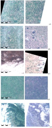
This study was carried out for five Sentinel-2 tiles in three countries: Argentina (Sentinel-2 tile grid numbers 20HNH and 20HPH), U.S.A. (14SKF) and Ukraine (36UUU, 34UFU) (see Figure 1 for examples). The selected tiles cover intensive agriculture regions, where changes are rapid due to seasonal crop development, and a mountain region in the Carpathians (tile 34UFU) where surface elevation varies approximately from 100 m to 1000 m. All selected regions feature considerable difference in Landsat-8 and Sentinel-2A image acquisition dates ranging from 4 July 2015 to 25 July 2016, as well as variable cloud conditions.

Figure 1. Examples of TOA true color images acquired by sentinel-2A/MSI (left) and Landsat-8/OLI (right): (A) tile 20HNH over Argentina, dates of Sentinel-2A/MSI and Landsat-8/OLI acquisitions are 2015358 and 2015361 respectively; (B) tile 20HPH over Argentina, acquisitions dates are 2015358 and 2015258; (C) tile 14SKF over Texas, U.S.A., dates of acquisitions are 2016012 and 2016104; (D) tile T36UUU over Ukraine, acquisition dates are 2016169 and 2016108; (E) tile T34UFU over the Carpathian Mountains, Ukraine, acquisitions dates are 2016198 and 2016063.

Overall co-registration of 45 Landsat-8 to Sentinel-2A pairs and 37 Sentinel-2A to Sentinel-2A pairs were analyzed. Table 1 gives details on the Landsat-8 and Sentinel-2A imagery used in the study.

Table 1. Description of data used in the study.

Country	Tile number	Acquisition date of Sentinel-2A reference image	Acquisition dates of Landsat-8 co-registered images	Acquisition dates of Sentinel-2A co-registered images
Argentina	20HNH	2015358	2015354, 2015185, 2015201, 2015242, 2015249, 2015258, 2015290, 2015306, 2015329, 2015338, 2015345, 2015361, 2016021, 2016037, 2016053	2015341, 2016006, 2016013, 2016016, 2016023, 2016026, 2016036, 2016043, 2016046, 2016063, 2016065, 2016073, 2016083, 2016093, 2016096
Argentina	20HPH	2015358	2015242, 2015258, 2015290, 2015306, 2015338, 2015354, 2016021, 2016037, 2016053	2016003, 2016013, 2016023, 2016043, 2016063, 2016073, 2016083, 2016093
US (Texas)	14SKF	2016012	2015245, 2015261, 2015293, 2015309, 2015325, 2015341, 2015357, 2016024, 2016040, 2016056, 2016072, 2016088, 2016104	2016042, 2016072, 2016132
Ukraine	36UUU	2016169	2016076, 2016092, 2016108, 2016156, 2016172, 2016188	2016096, 2016109, 2016119, 2016156, 2016166, 2016179, 2016196, 2016199, 2016206
Ukraine	34UFU	2016198	2016063, 2016182	2016048, 2016208

Note: Acquisition dates are given in the format YY YY DOY (where DOY is the day of the year).

3. Methodology

3.1. General overview

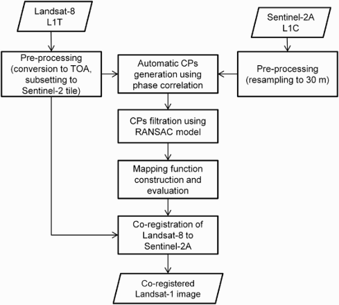
The proposed approach follows the general concept of automatic image-to-image registration outlined in (Zitova and Flusser 2003). It has the following steps (Figure 2): image pre-processing; automatic identification of CPs; filtering of CPs; building and evaluating a transformation, and image warping.

Figure 2. General workflow of Landsat-8 and Sentinel-2A image co-registration.

3.2. Image pre-processing

Landsat-8 images were converted from DNs to TOA reflectance values using calibration coefficients in the metadata file, so both Landsat-8 and Sentinel-2A images were generated with TOA reflectance values. The steps outlined in this and following subsections will also be valid, should co-registration be applied for atmospherically corrected products (Vermote et al. 2016).

For Landsat-8 to Sentinel-2A co-registration, Sentinel-2A band 08 (NIR) was resampled from 10 m to 30 m using averaging, and Landsat-8 data were subset to the corresponding Sentinel-2A tile using the nearest neighborhood resampling technique. Sentinel-2A to Sentinel-2A co-registration was performed at the original 10 m spatial resolution without further resampling.

3.3. Automatic generation of CPs

In this study, we exploited a phase-only correlation image matching method introduced by Guizar-Sicairos, Thurman, and Fienup (2008). It uses a cross-correlation approach in the frequency domain by means of the Fourier transform and exploits a computationally efficient procedure based on non-linear optimization and discrete Fourier transforms to detect sub-pixel shifts between reference and sensed images. For the detailed description of the algorithm, we refer readers to Guizar-Sicairos, Thurman, and Fienup (2008).

The phase-correlation algorithm allows detection of translation between reference and sensed images, and therefore is routinely applied using a moving square window. The size of the window and the step are selected empirically. Window size should be large enough to capture similarities on the reference and sensed images, and small enough to have a dense grid of CPs to accurately construct a transform function. In this study, window size and step were selected 100 and 50 pixels, respectively when co-registering Landsat-8 to Sentinel-2A, and 64 and 32 when co-registering multi-temporal Sentinel-2A images.

Compared to other area-based methods (e.g. cross-correlation in the spatial domain), the phase-correlation image usually contains a sharp peak corresponding to the dominant shift between images, and is usually more robust to temporal changes between reference and sensed images (Kravchenko, Lavrenyuk, and Kussul 2014). Compared to feature-based methods, the phase-correlation approach with a moving window allows detection of a dense grid of CPs, especially in cases where features cannot be reliably identified and detected, including at the 30 m spatial resolution imagery.

No matter what method is applied for automatic generation of CPs, filtering is necessary to remove unreliable CPs. First, a peak cross-correlation normalized magnitude is used for initial rejection of CPs. In our study, this value was set to 0.5. After that, a RANdom SAmple Consensus (RANSAC) algorithm (Fischler and Bolles 1981) is run for the linear transformation model to detect inliers and outliers. The RANSAC is a widely used algorithm in computer vision and image processing to detect strong outliers with large deviations (Brown and Lowe 2007). However, one should be careful to not aggressively remove outliers that can be actually inliers. In our study, we ran a conservative approach for removing outliers, that is, the RANSAC parameters were set in such a way to remove only outliers with a high confidence level. In our particular case, the number of RANSAC trials was set to 100, and a confidence level for selecting outliers was set to 0.99. The detected inlier CPs are further used to construct and evaluate a transformation function.

3.4. Transformation function

The goal of constructing a transformation function F() is to find correspondence between points in the reference image x_r = (x_r, y_r) and points in the sensed image x_s = (x_s, y_s):(1) Function F() is constructed using the set of CPs identified in the previous steps. In this study we compared three different approaches to creating the transformation function: polynomial models, RBFs and random forest (RF) regression trees (see below for details). Regardless of transformation approach, all available CPs were randomly split into a training (calibration) set (80%) and a testing set (20%). The training set was used to build the model and identify its parameters, while the testing set was used to evaluate the model on independent data. We will denote CPs from the testing set with and where and L is the number of points with corresponding shifts:(2) The quality of the transformation is evaluated using a RMSE between reference values and estimated values by transformation function F() using the testing set:(3) (4)

3.4.1. Polynomial models

Selection of the type of the transformation function depends on a-priori knowledge of expected geometric deformations and distortions between reference and sensed images, and required registration accuracy (Zitova and Flusser 2003). Polynomial functions of the n-th degree have the following form:(5) (6) In the case of n = 0, the models (5)–(6) are simple translation models where the same values of shift, namely and , are applied in x and y directions, respectively:(7) (8) A linear model, also referred to as affine, can be reduced to the following form:(9) (10) Model parameters and are estimated through the ordinary least square method, by minimizing the sum of the squares of the differences between predicted values of the model and reference values.

3.4.2. Radial basis functions

The transformation function based on RBFs has the following form (Zitova and Flusser 2003):(11) (12) where is the kernel function with parameters (centers) and and weights and .

In this study, we used two types of kernels, namely Gaussian and thin-plate splines (TPS):(13) (14) There are several ways of selecting a set of centers : randomly, on a regular grid, or adaptively through clustering. We used the k-means clustering approach (Forgy 1965; Lloyd 1982) to adaptively select centers in the models (11)–(12). We varied number of clusters K and found values from 1 to 10 producing best results. Increasing the number over 10 did not improve results.

And finally, weights and in models (11)–(12) were estimated from training data using the RANSAC algorithm (Fischler and Bolles 1981).

As with polynomial models, RBF models are the global mapping functions, however, they are able to account for local non-linear distortions (Zitova and Flusser 2003).

3.4.3. RF regression

RF is a machine learning algorithm that represents an ensemble of decision trees (DTs) (Breiman 2001). A DT classifier or regression model is built from a set of data using the concept of information entropy. At each node of the tree, one attribute of the data, that most effectively splits its set of samples into subsets enriched in one class or the other, is selected. Its criterion is the normalized information gain that results from choosing an attribute for splitting the data. The attribute with the highest normalized information gain is chosen to make the decision. The algorithm then recurs on the smaller sublists. One disadvantage of the DT classifier is the considerable sensitivity to the input dataset, so that a small change to the training data can result in a very different set of subsets (Bishop 2006). In order to overcome disadvantages of a single DT, an ensemble of DTs is used to form a RF. Each DT represents an independent expert (or weak classifier) in the RF that is trained based on different input datasets that are generated through a bagging procedure (Bishop 2006). RF can be used for building classification and regression models.

In this study, the RF regression was used to build a transformation function. We used points from the reference image x_r = (x_r, y_r) as inputs to the RF regression model with a polynomial pre-processing. For example, in case of the 2nd degree polynomial function, the following features were input to the RF model: . The RF model was further trained to predict points in the sensed image x_s = (x_s, y_s). In this study, the number of DTs in the RF models was kept low (about 5) to avoid overfitting. The optimal number of DTs in the RF model in terms of RMSE error was identified through the cross-validation procedure.

As with RBFs based mapping functions, RF belongs to the class of global mapping models that can account for local non-linear distortions.

4. Results

The use of phase correlation allowed us to generate hundreds and thousands of CPs when co-registering Landsat-8 to Sentinel-2A at 30 m spatial resolution (hereafter referred as LandSen30), and when co-registering multi-temporal Sentinel-2A images at 10 m spatial resolution (hereafter referred as SenSen10) (Figure 3). The average misregistration between Landsat-8 and Sentinel-2A calculated on a tile basis, using identified CPs, varied from 0.11 pixels to 1.35 pixels among tiles considered in the study with the maximum misregistration value varying from 0.25 to 1.59 pixels (per tile). Misregistration between Landsat-8 and Sentinel-2A was stable in time over the same tile (Table 2, Figure 4) with average standard deviation of the misregistration through the time varying from 0.03 pixels to 0.16 pixels with average of 0.10 pixels (at 30 m resolution).

Figure 3. Location of CPs shown in the form of vectors outlining the direction and magnitude of shifts ( and (Equation (2)) found between Landsat-8 image acquired on 2016021 (21-Jan-2016), and Sentinel-2A image acquired on 2015358 (24-Dec-2015) and used as a reference image, over the study area in Argentina, tile T20HNH. Vector lengths were multiplied by 100 for visual clarity. Overall, 1634 CPs were found using the phase-correlation approach in this case. The background is a Landsat-8 TOA NIR (band 5) image with TOA reflectance values scaled from 0.05 to 0.65.

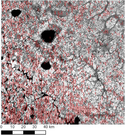
Figure 4. Distribution of misregistration values and (Equation (2)) when co-registering Landsat-8 to Sentinel-2A images for different tiles used in the study. Units are shown in pixel values at 30 m spatial resolution.

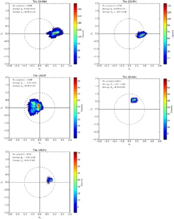
Table 2. Results of identifying CPs on the sensed (Landsat-8) and reference (Sentinel-2A) images using phase-correlation approach at 30 m spatial resolution.

Tile	Date of sensed image acquisition	Number of CPs	mean	std	min	max	mean	std	min	max
20HNH	2015185	694	1.15	0.08	0.96	1.34	0.24	0.06	0.12	0.35
	2015201	652	1.18	0.11	0.85	1.46	0.22	0.08	0	0.45
	2015242	718	0.91	0.09	0.74	1.07	0.04	0.05	−0.07	0.13
	2015249	512	1.14	0.11	0.88	1.34	0.13	0.06	−0.03	0.25
	2015258	679	0.97	0.13	0.63	1.31	0.03	0.05	−0.1	0.16
	2015290	939	0.98	0.09	0.72	1.23	−0.01	0.08	−0.24	0.17
	2015306	810	0.99	0.08	0.8	1.17	0.02	0.05	−0.1	0.19
	2015329	454	1.34	0.11	1.02	1.59	0.05	0.09	−0.16	0.28
	2015338	1854	1	0.09	0.76	1.25	−0.03	0.11	−0.31	0.2
	2015345	866	1.22	0.05	1.1	1.35	0.14	0.02	0.08	0.19
	2015354	2338	0.96	0.13	0.59	1.32	−0.03	0.07	−0.24	0.13
	2015361	1268	1.22	0.06	1.08	1.36	0.07	0.04	−0.03	0.16
	2016021	1419	0.96	0.11	0.69	1.27	0.01	0.06	−0.17	0.18
	2016037	1017	0.95	0.12	0.6	1.29	0.12	0.07	−0.06	0.29
	2016053	876	0.81	0.15	0.41	1.19	0.08	0.06	−0.07	0.21
20HPH	2015242	726	0.88	0.11	0.53	1.14	−0.06	0.07	−0.27	0.1
	2015258	652	0.93	0.13	0.54	1.19	−0.01	0.05	−0.13	0.09
	2015290	848	0.89	0.1	0.56	1.13	−0.08	0.07	−0.27	0.06
	2015306	709	0.98	0.07	0.73	1.16	−0.03	0.04	−0.17	0.06
	2015338	2637	0.79	0.12	0.46	1.08	−0.09	0.07	−0.28	0.07
	2015354	2912	0.82	0.11	0.53	1.08	−0.13	0.07	−0.3	0.04
	2016021	1634	0.77	0.1	0.5	1	−0.08	0.07	−0.28	0.09
	2016037	1070	0.82	0.1	0.54	1.05	0.02	0.07	−0.18	0.18
	2016053	574	0.71	0.11	0.41	0.91	0	0.07	−0.21	0.16
36UUU	2016076	770	0.28	0.08	0.08	0.47	0.6	0.07	0.44	0.76
	2016092	695	0.33	0.1	0.08	0.62	0.58	0.06	0.41	0.73
	2016108	856	0.29	0.09	0.1	0.55	0.6	0.06	0.45	0.79
	2016156	796	0.27	0.09	0.08	0.51	0.57	0.06	0.38	0.72
	2016172	2379	0.31	0.08	0.14	0.5	0.6	0.05	0.46	0.73
	2016188	818	0.37	0.07	0.2	0.55	0.61	0.06	0.39	0.75
14SKF	2015245	721	−0.45	0.14	−0.75	−0.12	0.13	0.1	−0.09	0.39
	2015261	472	−0.43	0.18	−0.89	0.01	0.05	0.11	−0.22	0.37
	2015293	721	−0.48	0.14	−0.76	−0.06	−0.24	0.11	−0.53	0.12
	2015309	1195	−0.38	0.13	−0.65	−0.05	0.36	0.08	0.18	0.55
	2015325	1095	−0.38	0.14	−0.67	−0.04	−0.12	0.12	−0.49	0.19
	2015341	703	−0.03	0.08	−0.21	0.22	0.06	0.06	−0.06	0.18
	2015357	1100	−0.36	0.14	−0.65	0	−0.16	0.1	−0.42	0.12
	2016024	729	−0.05	0.11	−0.28	0.26	0.11	0.09	−0.11	0.32
	2016040	1258	−0.05	0.09	−0.23	0.19	−0.08	0.07	−0.29	0.11
	2016056	1117	−0.39	0.12	−0.66	−0.08	0.33	0.09	0.12	0.6
	2016072	752	−0.05	0.08	−0.24	0.18	0.19	0.06	0.02	0.34
	2016088	1085	−0.37	0.1	−0.59	−0.08	0.14	0.08	−0.04	0.36
	2016104	992	−0.06	0.08	−0.22	0.16	0.19	0.07	0.01	0.4
34UFU	2016063	636	0.61	0.07	0.46	0.78	0.15	0.1	−0.16	0.46
	2016182	1498	0.76	0.04	0.66	0.87	0.14	0.05	0.05	0.29

Note: Values for shifts and (Equation (2)) are shown in pixel units.

In the SenSen10 case, performance depended on whether the reference and sensed Sentinel-2A images were acquired from the same or different (adjacent) orbits. In case of the same orbits, the average misregistration calculated on a tile basis varied from 0.05 pixels to 0.46 pixels among tiles (with the maximum misregistration up to 1.21 pixels) with average 0.23 ± 0.12 pixels at 10 m resolution (Table 3, Figure 5). In case of different Sentinel-2 orbits over the same tile, the average misregistration calculated on a tile basis varied from 0.14 pixels to 1.45 pixels among tiles (with the maximum misregistration up to 2.83 pixels) with average 0.61 ± 0.42 pixels at 10 m resolution (Table 3, Figure 6). This might be the result of the satellite yaw bias that was corrected within the recent baseline processing version 02.04 (ESA 2016a). Overall, our estimates of the multi-temporal misregistration in the Sentinel-2A imagery were consistent with the Sentinel-2 Data Quality Reports (ESA 2016a).

Figure 5. Distribution of misregistration values and when co-registering multi-temporal Sentinel-2A images from the same orbits for different tiles used in the study. Units are shown in pixel values at 10 m spatial resolution.

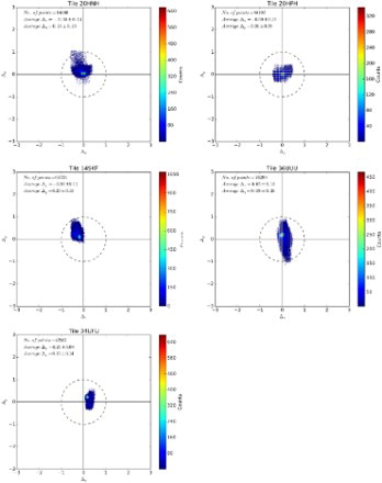
Figure 6. Distribution of misregistration values and when co-registering multi-temporal Sentinel-2A images from the adjacent orbits for different tiles used in the study. Units are shown in pixel values at 10 m spatial resolution.

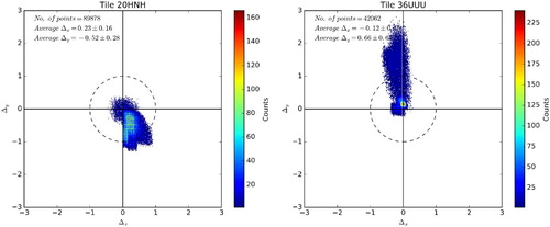
Table 3. Results of identifying CPs on the sensed (Sentinel-2A) and reference (Sentinel-2A) images using phase-correlation approach at 10 m spatial resolution.

	Date of sensed image acquisition (baseline processing version, orbit relative to the orbit of reference image)
Tile		Number of CPs	mean	std	min	max	mean	std	min	max
20HNH	2016013 (v02.01, same)	20622	−0.03	0.04	−0.16	0.08	0.04	0.04	−0.04	0.15
	2016023 (v02.01, same)	21934	0.06	0.04	−0.04	0.16	0.05	0.04	−0.06	0.15
	2016043 (v02.01, same)	15453	−0.03	0.06	−0.17	0.1	0.02	0.06	−0.13	0.18
	2016063 (v02.01, same)	6133	0.12	0.11	−0.37	0.41	0.19	0.12	−0.14	0.45
	2016073 (v02.01, same)	12919	−0.11	0.07	−0.23	0.03	0.21	0.1	−0.03	0.48
	2016083 (v02.01, same)	13439	−0.27	0.11	−0.6	0.03	0.11	0.1	−0.18	0.42
	2016093 (v02.01, same)	4160	−0.16	0.17	−0.61	0.31	0.35	0.31	−0.54	1.09
	2015341 (v02.00, adjacent)	15056	0.22	0.09	0	0.43	−0.42	0.19	−0.93	0.12
	2016006 (v02.01, adjacent)	17858	0.08	0.04	−0.01	0.16	−0.76	0.18	−1.2	−0.3
	2016016 (v02.01, adjacent)	18265	0.24	0.08	0.05	0.44	−0.6	0.3	−1.3	0.15
	2016026 (v02.01, adjacent)	16795	0.41	0.18	−0.12	0.92	−0.53	0.24	−1.15	0.1
	2016036 (v02.01, adjacent)	2281	−0.04	0.12	−0.34	0.28	−0.05	0.16	−0.42	0.34
	2016046 (v02.01, adjacent)	8566	0.3	0.14	−0.08	0.68	−0.34	0.15	−0.69	0
	2016065 (v02.01, adjacent)	9997	0.23	0.12	−0.01	0.49	−0.36	0.23	−1.04	0.33
	2016096 (v02.01, adjacent)	1060	−0.02	0.17	−0.47	0.47	0.02	0.16	−0.35	0.4
20HPH	2016003 (v02.01, same)	2286	0.01	0.15	−0.35	0.38	0	0.14	−0.42	0.47
	2016013 (v02.01, same)	29887	0	0.04	−0.08	0.08	0.01	0.04	−0.08	0.11
	2016023 (v02.01, same)	20264	0.07	0.05	−0.05	0.19	0	0.06	−0.18	0.15
	2016043 (v02.01, same)	10197	−0.04	0.07	−0.24	0.19	−0.01	0.07	−0.19	0.21
	2016063 (v02.01, same)	7065	0.24	0.12	−0.02	0.51	0.15	0.11	−0.18	0.45
	2016073 (v02.01, same)	7492	−0.09	0.07	−0.27	0.12	0.03	0.07	−0.12	0.17
	2016083 (v02.01, same)	9020	−0.24	0.08	−0.43	−0.05	−0.07	0.11	−0.35	0.22
	2016093 (v02.01, same)	1981	−0.06	0.15	−0.39	0.25	0.05	0.17	−0.38	0.47
36UUU	2016109 (v02.01, same)	18989	0.18	0.12	−0.16	0.47	0.2	0.24	−0.5	0.93
	2016119 (v02.01, same)	21363	0.08	0.11	−0.26	0.45	−0.17	0.29	−1.16	0.61
	2016179 (v02.04, same)	19300	0	0.04	−0.08	0.08	0.21	0.05	0.08	0.33
	2016199 (v02.04, same)	16647	−0.07	0.06	−0.24	0.08	0.14	0.06	−0.03	0.3
	2016096 (v02.01, adjacent)	10046	−0.1	0.13	−0.47	0.29	1.44	0.51	−0.13	2.82
	2016156 (v02.02, adjacent)	8145	−0.32	0.13	−0.68	0.1	1.19	0.4	−0.04	2.02
	2016166 (v02.02, adjacent)	10436	0.01	0.04	−0.09	0.14	0.13	0.05	−0.02	0.24
	2016196 (v02.04, adjacent)	8530	−0.06	0.07	−0.22	0.08	0.25	0.08	0.01	0.47
	2016206 (v02.04, adjacent)	4905	−0.17	0.09	−0.38	0.07	0	0.08	−0.23	0.2
14SKF	2016042 (v02.01, same)	28459	−0.17	0.04	−0.27	−0.05	0.1	0.06	−0.02	0.22
	2016072 (v02.01, same)	19183	−0.37	0.09	−0.56	−0.13	0.21	0.09	−0.08	0.45
	2016132 (v02.01, same)	18091	−0.26	0.1	−0.58	0.05	0.35	0.17	−0.22	0.94
34UFU	2016048 (v02.01, same)	16528	0.28	0.08	0.06	0.55	0.05	0.18	−0.37	0.61
	2016208 (v02.04, same)	26453	0.16	0.03	0.06	0.25	0.22	0.04	0.08	0.33

Note: Values for shifts and (Equation (2)) are shown in pixel units.

When building a transformation function, all considered approaches showed a similar performance (Tables 4–6) with the complex non-linear RF regression slightly outperforming other methods, namely, a simple translation (Equations (7)–(8)), 1st order polynomial (Equations (9)–(10)), Gaussian RBFs (Equations (11)–(12), (13)) and TPS (Equations (11)–(12), (14)). For the RF regression, RMSE values varied from 0.02 to 0.12 pixels for the LandSen30 case at 30 m resolution, and from 0.025 to 0.22 pixels for the SenSen10 case at 10 m resolution for the same orbits and from 0.05 to 0.26 pixels for adjacent orbits. The RF model was built using a 1st order polynomial function for input CP coordinates. Increasing the order of the polynomial function did not improve performance of the RF model. It means that the RF was able to capture non-linearity when building a transformation function between CPs on the reference and sensed images.

Table 4. Average and standard deviation of the RMSE error (Equation (4)) calculated for different transformation functions using CPs from testing set when co-registering Landsat-8 and Sentinel-2A images.

	Translation (Equations (7)–(8))		1st order polynomial (Equations (9)–(10))		Gaussian RBFs (Equations (11)–(12), (13))		RF regression		TPS (Equations (11)–(12), (14))
Tile	Mean	Standard deviation	Mean	Standard deviation	Mean	Standard deviation	Mean	Standard deviation	Mean	Standard deviation
20HNH	0.119	0.031	0.091	0.026	0.093	0.027	0.084	0.024	0.090	0.025
20HPH	0.123	0.014	0.078	0.016	0.081	0.017	0.073	0.018	0.079	0.018
36UUU	0.108	0.011	0.072	0.015	0.074	0.015	0.059	0.014	0.073	0.015
14SKF	0.145	0.037	0.094	0.018	0.095	0.018	0.074	0.018	0.094	0.017
34UFU	0.095	0.045	0.056	0.034	0.060	0.038	0.044	0.030	0.054	0.033

Note: RMSE values are shown in pixel units at 30 m spatial resolution.

Table 5. Average and standard deviation of the RMSE error (Equation (4)) calculated for different transformation functions using CPs from testing set when co-registering multi-temporal Sentinel-2A images from the same orbit.

	Translation (Equations (7)–(8))		1st order polynomial (Equations (9)–(10))		Gaussian RBFs (Equations (11)–(12), (13))		RF regression		TPS (Equations (11)–(12), (14))
Tile	Mean	Standard deviation	Mean	Standard deviation	Mean	Standard deviation	Mean	Standard deviation	Mean	Standard deviation
20HNH	0.141	0.104	0.125	0.076	0.125	0.076	0.105	0.060	0.126	0.074
20HPH	0.133	0.064	0.128	0.062	0.127	0.062	0.114	0.059	0.129	0.064
36UUU	0.181	0.126	0.114	0.046	0.114	0.046	0.088	0.035	0.112	0.048
14SKF	0.133	0.066	0.123	0.050	0.118	0.046	0.089	0.036	0.123	0.051
34UFU	0.122	0.101	0.092	0.086	0.091	0.084	0.066	0.059	0.093	0.088

Note: RMSE values are shown in pixel units at 10 m spatial resolution.

Table 6. The same as Table 5, but for adjacent Sentinel-2A orbits.

	Translation (Equations (7)–(8))		1st order polynomial (Equations (9)–(10))		Gaussian RBFs (Equations (11)–(12), (13))		RF regression		TPS (Equations (11)–(12), (14))
Tile	Mean	Standard deviation	Mean	Standard deviation	Mean	Standard deviation	Mean	Standard deviation	Mean	Standard deviation
20HNH	0.239	0.048	0.207	0.031	0.202	0.028	0.164	0.032	0.205	0.031
36UUU	0.248	0.212	0.191	0.139	0.189	0.138	0.138	0.087	0.193	0.142

Our results obtained for the 1st order polynomial function were comparable to previous studies by Barazzetti, Cuca, and Previtali (2016) and Yan et al. (2016).

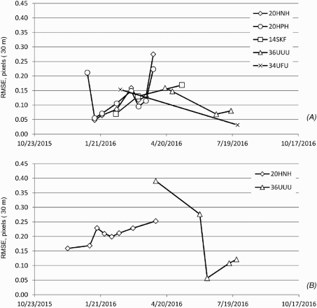
Temporal fluctuations of the RMSE error were analyzed to explore temporal stability of the constructed transformation functions for multi-temporal Sentinel-2A images co-registration. Figure 7 shows dependence of the RMSE error with time for the 1st degree polynomial function for different Sentinel-2A orbits. For the case of the same orbits, there are not too many variations in time, except three cases with RMSE values over 0.2 pixels. These are due to heavy cloud contamination presented in the sensed imagery. As to the adjacent orbits, the tile T20HNH shows a trend which is due to the difference between the sensed and reference images: the difference is up to 103 days. For the T36UUU case, high RMSE error can be attributed to the 70 day difference between the reference and sensed images acquired over highly intensive agriculture region that features a lot of changes within this time period (Figure 1 (D)). Also, reduction of the RMSE error for 36UUU tile comparing to the 20HNH tile can be related to the improvements made in the baseline processing version 02.04 (ESA 2016a).

Figure 7. Changes of RMSE error of building a 1st degree polynomial transformation function when registering multi-temporal Sentinel-2A images over the time for different tiles and different Sentinel-2A orbits: (A) same orbits; (B) adjacent orbits.

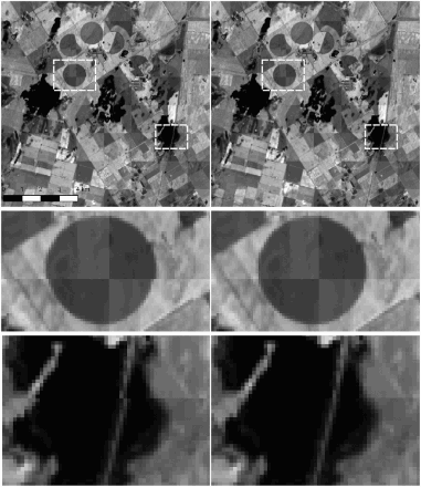
Results on correcting misregistration between Landsat-8 and Sentinel-2A are shown in Figure 8.

Figure 8. A 30 m ‘chessboard’ composed of alternating Landsat-8 (acquired on 20-Dec-2015) and Sentinel-2A (24-Dec-2015) images before (left panel) and after co-registration (right panel). Near-infrared images from band 5 (Landsat-8) and band 8 (Sentinel-2A) were used to produce these ‘chessboard’. TOA reflectance values were scaled from 0.05 to 0.55. This subset covers the area in the south-east part of the tile 20HNH over Argentina (Figure 1(A)). Misregistrations between satellite images can be seen in the irrigated fields (circles, middle left image) and in the bridge over the lake (bottom left image) with corrections applied and misregistration disappearing in the right images (middle and bottom). Middle and bottom subset images are shown in corresponding boxes on the top images.

The proposed workflow was implemented in Python programming language using the Geospatial Data Abstraction Library (GDAL) for managing geospatial datasets, the ‘skimage package’ for phase-correlation implementation, and the ‘sklearn package’ for the RF regression and RANSAC implementations, and was computationally efficient. Typical processing times on the Dell Laptop with processor Inter® Core™ i7-4810MQ CPU @ 2.80 GHz with 16 Gb RAM are presented in Table 7.

Table 7. Typical processing times (in seconds) for the main steps of the proposed approach.

Processing step	SenSen10	LandSen30
CPs identification	135	22
Precomputing shifts with 1st order polynomial function	5	0.5
Precomputing shifts with the RF regression	220	8
Warping (single scene)	210	25

5. Conclusions

Since many applications involving satellite imagery require the use of multi-temporal datasets, misregistration issues can lead to incorrect results. This study investigated misregistration issues between Landsat-8/OLI and Sentinel-2A/MSI at 30 m resolution, and between multi-temporal Sentinel-2A images at 10 m resolution using a phase-correlation approach and multiple transformation functions. Phase correlation proved to be a robust approach that allowed us to identify hundreds and thousands of control points on images acquired more than 100 days apart. Overall, misregistration of up to 1.6 pixels at 30 m resolution between Landsat-8 and Sentinel-2A images, and 1.2 pixels (for the same orbit) and 2.8 pixels (for different orbits) at 10 m resolution between multi-temporal Sentinel-2A images were observed. The non-linear RF regression used for constructing the mapping function showed best results in terms of error, yielding the average RMSE error of 0.07 ± 0.02 pixels at 30 m resolution and 0.09 ± 0.05 and 0.15 ± 0.06 pixels at 10 m resolution for the same and adjacent Sentinel-2A orbits, respectively, for multiple tiles and multiple conditions. On the other hand, a simple linear model such as 1st order polynomial function can provide an error of up to 0.08 ± 0.02 pixels at 30 m resolution and 0.12 ± 0.06 (same Sentinel-2A orbits) and 0.20 ± 0.09 (adjacent orbits) pixels at 10 m resolution.

Disclosure statement

No potential conflict of interest was reported by the authors.

ORCID

Sergii Skakun http://orcid.org/0000-0002-9039-0174

References

- Barazzetti, L., B. Cuca, and M. Previtali. 2016. “Evaluation of Registration Accuracy Between Sentinel-2 and Landsat 8.” In Fourth International Conference on Remote Sensing and Geoinformation of the Environment, 968809–968809. International Society for Optics and Photonics. doi:10.1117/12.2241765.
- Bishop, C. M. 2006. Pattern Recognition and Machine Learning. New York: Springer.
- Breiman, L. 2001. “Random Forests.” Machine Learning 45 (1): 5–32. doi:10.1023/A:1010933404324.
- Brown, M., and D. G. Lowe. 2007. Automatic Panoramic Image Stitching Using Invariant Features.” International Journal of Computer Vision 74 (1): 59–73. doi:10.1007/s11263-006-0002-3.
- Dechoz, C., V. Poulain, S. Massera, F. Languille, D. Greslou, F. de Lussy, A. Gaudel, C. L’Helguen, C. Picard, and T. Trémas. 2015. “Sentinel 2 Global Reference Image.” In SPIE Remote Sensing, pp. 96430A-96430A. International Society for Optics and Photonics. doi:10.1117/12.2195046.
- Drusch, M., U. Del Bello, S. Carlier, O. Colin, V. Fernandez, F. Gascon, B. Hoersch, et al. 2012. “Sentinel-2: ESA’s Optical High-Resolution Mission for GMES Operational Services.” Remote Sensing of Environment 120: 25–36. doi:10.1016/j.rse.2011.11.026.
- ESA. 2016a. “ S2 MPC. Data Quality Report.” Ref: S2-PDGS-MPC-DQR, Issue: 08, Date: 05/10/2016. https://earth.esa.int/documents/247904/685211/Sentinel-2-Data-Quality-Report.
- ESA. 2016b. “ Sentinel-2 Products Specification Document.” Ref: S2-PDGS-TAS-DI-PSD, Issue: 14.0, Date: 15/07/2016. https://earth.esa.int/web/sentinel/user-guides/sentinel-2-msi/document-library.
- Fischler, M. A., and R. C. Bolles. 1981. “Random Sample Consensus: A Paradigm for Model Fitting with Applications to Image Analysis and Automated Cartography.” Communications of the ACM 24 (6): 381–395. doi:10.1145/358669.358692.
- Forgy, E. W. 1965. “Cluster Analysis of Multivariate Data: Efficiency Versus Interpretability of Classifications.” Biometrics 21: 768–769.
- Gao, F., J. Masek, and R. E. Wolfe. 2009. “Automated Registration and Orthorectification Package for Landsat and Landsat-Like Data Processing.” Journal of Applied Remote Sensing 3 (1): 033515–033515. doi:10.1117/1.3104620.
- Guizar-Sicairos, M., S. T. Thurman, and J. R. Fienup. 2008. “Efficient Subpixel Image Registration Algorithms.” Optics Letters 33 (2): 156–158. doi:10.1364/OL.33.000156.
- Gutman, G., C. Huang, G. Chander, P. Noojipady, and J. G. Masek. 2013. “Assessment of the NASA–USGS Global Land Survey (GLS) Datasets.” Remote Sensing of Environment 134: 249–265. doi:10.1016/j.rse.2013.02.026.
- Ju, J., and J. G. Masek. 2016. “The Vegetation Greenness Trend in Canada and US Alaska From 1984–2012 Landsat Data.” Remote Sensing of Environment 176: 1–16. doi:10.1016/j.rse.2016.01.001.
- Justice, C., G. Gutman, and K. P. Vadrevu. 2015. “NASA Land Cover and Land Use Change (LCLUC): An Interdisciplinary Research Program.” Journal of Environmental Management 148: 4–9. doi:10.1016/j.jenvman.2014.12.004.
- Kravchenko, O., M. Lavrenyuk, and N. Kussul. 2014. “Orthorectification of Sich-2 Satellite Images Using Elastic Models.” In 2014 IEEE Geoscience and Remote Sensing Symposium, 2281–2284. IEEE. doi:10.1109/IGARSS.2014.6946925.
- Le Moigne, J., N. S. Netanyahu, and R. D. Eastman. 2011. Image Registration for Remote Sensing. Cambridge: Cambridge University Press.
- Lloyd, S. 1982. “Least Squares Quantization in PCM.” IEEE Transactions on Information Theory 28 (2): 129–137. doi:10.1109/TIT.1982.1056489.
- Roy, D. P., J. Ju, K. Kline, P. L. Scaramuzza, V. Kovalskyy, M. Hansen, T. R. Loveland, E. Vermote, and C. Zhang. 2010. “Web-enabled Landsat Data (WELD): Landsat ETM+ Composited Mosaics of the Conterminous United States.” Remote Sensing of Environment 114 (1): 35–49. doi:10.1016/j.rse.2009.08.011.
- Roy, D. P., M. A. Wulder, T. R. Loveland, C. E. Woodcock, R. G. Allen, M. C. Anderson, D. Helder, et al. 2014. “Landsat-8: Science and Product Vision for Terrestrial Global Change Research.” Remote Sensing of Environment 145: 154–172. doi:10.1016/j.rse.2014.02.001.
- Shelestov, A., M. Lavreniuk, N. Kussul, A. Novikov, and S. Skakun. 2017. “Exploring Google Earth Engine Platform for Big Data Processing: Classification of Multi-Temporal Satellite Imagery for Crop Mapping.” Frontiers in Earth Science 5 (17): 1–7. doi:10.3389/feart.2017.00017.
- Skakun, S., N. Kussul, A. Y. Shelestov, M. Lavreniuk, and O. Kussul. 2016. “Efficiency Assessment of Multitemporal C-Band Radarsat-2 Intensity and Landsat-8 Surface Reflectance Satellite Imagery for Crop Classification in Ukraine.” IEEE Journal of Selected Topics in Applied Earth Observations and Remote Sensing 9 (8): 3712–3719. doi:10.1109/JSTARS.2015.2454297.
- Storey, J., M. Choate, and K. Lee. 2014. “Landsat 8 Operational Land Imager on-Orbit Geometric Calibration and Performance.” Remote Sensing 6 (11): 11127–11152. doi:10.3390/rs61111127.
- Storey, J., D. P. Roy, J. Masek, F. Gascon, J. Dwyer, and M. Choate. 2016. “A Note on the Temporary Misregistration of Landsat-8 Operational Land Imager (OLI) and Sentinel-2 Multi Spectral Instrument (MSI) Imagery.” Remote Sensing of Environment 186: 121–122. doi:10.1016/j.rse.2016.08.025.
- Vermote, E., C. Justice, M. Claverie, and B. Franch. 2016. “Preliminary Analysis of the Performance of the Landsat 8/OLI Land Surface Reflectance Product.” Remote Sensing of Environment 185: 46–56. doi:10.1016/j.rse.2016.04.008.
- Yan, L., D. P. Roy, H. Zhang, J. Li, and H. Huang. 2016. “An Automated Approach for Sub-Pixel Registration of Landsat-8 Operational Land Imager (OLI) and Sentinel-2 Multi Spectral Instrument (MSI) Imagery.” Remote Sensing 8 (6): 520. doi:10.3390/rs8060520.
- Zitova, B., and J. Flusser. 2003. “Image Registration Methods: A Survey.” Image and Vision Computing 21 (11): 977–1000. doi:10.1016/S0262-8856(03)00137-9.