On the surface fluxes characteristics and roughness lengths at Zhongshan station, Antarctica

ABSTRACT

Over Antarctica, surface fluxes play an important role in the local atmospheric dynamical processes. To reveal the surface fluxes characteristics and aerodynamic and thermal roughness lengths over Zhongshan station, Antarctica, this paper analyzes the data observed at the station during 3 March 2008 through 15 February 2009. It is found that easterlies dominated this site throughout the whole year, with a maximum (average) speed of 25 (5.6) m s⁻¹ at 3.9 m height, and the annual maximum (minimum) surface temperature reached 291.05 (230.05) K, while the annual maximum (minimum) air-specific humidity was 4.1 (0.05) g/kg at 3.9 m height. The maximum (minimum) values of seasonal mean temperature, humidity, each radiation components, sensible and latent heat flux occurred in summer (winter), while for the seasonal averaged wind speed and τ the minimums (maximums) appeared in summer (autumn). After comparing with a partially linear regression method for aerodynamic roughness length and four previous equations that derive thermal roughness length from surface Reynolds number, constant values of aerodynamic roughness length as 3.6 × 10⁻³m and thermal roughness length as 1.2 × 10⁻⁴m at this site were validated by using the other three level observations and suggested for future studies.

KEYWORDS:

• Antarctica
• Zhongshan station
• turbulent momentum flux
• sensible heat flux
• aerodynamic roughness length
• thermal roughness length

1. Introduction

Antarctica is one of the most important systems which interact with the global circulation and climate (Gillett and Thompson 2003; Schneider, Steig, and Comiso 2004; Hendon, Thompson, and Wheeler 2007). However, Antarctica is also one of the coldest places on Earth, which makes surface observation over this region strictly difficult. To gather the meteorological data over this place, meteorological observations started at early twentieth century. In the recent 60 years starting from the first International Geophysical Year in 1957, more than 60 countries have set their Antarctica science research stations and carried out several observation projects. China operated Zhongshan station in Antarctica since 1989, and started to carry out flux observation by eddy covariance method here since 2007 (Lin et al. 2009).

Previous studies point out that, to successfully simulate the local atmospheric dynamical processes such as Antarctic atmospheric circulation and katabatic winds, surface fluxes parameterization is of great importance (e.g. Cassano, Parish, and King 2000; King, Connolley, and Derbyshire 2001; Guo, Bromwich, and Cassano 2002). In the current numerical models, surface fluxes parameterizations are mostly based on Monin–Obukhov similarity theory (MOST), which uses the averaged wind, temperature and humidity to calculate the momentum, sensible and latent heat fluxes. However, with the MOST, the calculated fluxes are sensitive to the choice of the aerodynamic roughness length (z₀m), roughness lengths for heat (z₀h) and moisture (z_0q). Using 45 months of observations from Hally, Antarctica, Cassano, Parish, and King (2000) found that, by changing z₀h from 1.1 × 10⁻⁴ to 8.0 × 10⁻³m the accuracy of sensible heat flux calculation was improved significantly. Reijmer, Meijgaard, and Broeke (2003) presented that different z₀m and z₀h settings could yield the 10-m wind speed difference of 10 ms⁻¹ and near-surface temperature difference of 10 K for one month regional climate model simulation. Vignon et al. (2017) found that using a constant value of z₀m would result in a significant friction velocity (u_*) error of 21%, which was related to the inhomogeneity caused by the orientation of the sastrugi.

For Zhongshan station, Qu and Gao (1996) found that z₀m was 2.9 × 10⁻²m by interpolating the wind profiles observed by a tethersonde meteorological tower, while for an ice sheet nearby Zhongshan station, Bian, Lu, and Jia (1997) and Lin et al. (2009) found that z₀m was about 4.3–4.6 × 10⁻⁴m. To the best knowledge of the authors, no report of z₀h at Zhongshan station was published so far. This paper first describes the observational data and methods used to derive fluxes in Section 2. Then, in Section 3 we present the results, including the general meteorological condition, radiation and turbulent fluxes characteristics, and the obtained roughness lengths. At last, summary and conclusions are given in Section 4.

2. Observational data and methods

2.1. Observation site and data

Zhongshan station is located at the Larsemann Hills of East Antarctica, at 69°22′S, 76°22′E, and north of the Grove mountains, south of the Prydz bay. It is within 2 km edge of the Antarctic ice sheet (Figure 1). At Zhongshan station, a meteorological tower was constructed, and a barometric pressure sensor CS100 by Apogee Instruments, an Infrared Radiometer IRR-P by Campbell Scientific Incorporation and a net radiometer CNR1 by Kipp & Zonen were installed at 3 m to collect air pressure, surface temperature and radiation data, respectively. WindSonic by Gill Instruments Limited and HMP45C by Campbell Scientific Incorporation were installed at 2.5, 3.9 and 5.9 m levels to observe wind, temperature and humidity, respectively. The observation frequency of these instruments are 0.1 Hz, and the data were averaged every 10 min. Three Dimensional Ultrasonic Anemometer CSAT-3 by Campbell Scientific Incorporation and Open Path CO₂/H₂O Infrared Gas Analyzer LI-7500 by LI-COR Incorporation were installed at 3.7 m height, with an observation frequency of 10 Hz. These observation instruments were all reliable under low temperature condition. Detailed description about the accuracy of the instruments can be found in Table 1 (Li et al. 2010). Consecutive observations were carried out from 3 March 2008 to 15 February 2009, and the quality control for the data was carried out as follows:

1. The spikes in the data series are removed by using a criterion of $X\left(t\right)<(\overline{X}-4\sigma )$ or $X\left(t\right)>(\overline{X}+4\sigma )$, where $X\left(t\right)$ denotes the measurements, $\overline{X}$ is the mean over the interval and $\sigma$ is the standard deviation. The interval is set to 24 h for 0.1 Hz observation and 10 min for the 10 Hz observation, respectively. The missing data are then interpolated linearly.

2. Fluxes were calculated by the eddy covariance method with 10 min averaging period. Linear detrending was first applied to the 10 Hz observations with 10 min interval (Moncrieff et al. 2005), and then covariances were calculated and adjusted by double rotation and WPL correction (Webb, Pearman, and Leuning 1980) to obtain the fluxes.

3. During the calculation of z₀m and z₀h, the data that u_* < 0.02 m s⁻¹ or the absolute value of sensible heat < 10 W m⁻² were omitted.

Figure 1. The (a) geographical location, (b) local topography and (c) the observation tower of Zhongshan station.

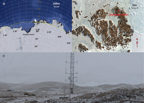
Table 1. The type of sensors and their key technical indexes.

Sensor type	Measurement range	Precision accuracy
CS100	P: 600–1100 hPa	< 0.5 hPa
IRR-P	Ts: −55∼ + 80°C	± 0.2°C (−15∼ + 60°C) ± 0.5°C (−55∼ + 80°C)
CNR1	DSR,USR : 0.3–3.0 µm DLR,ULR : 5–50 µm	10–35 µν/(wm^2) 5–35 µν/(wm^2)
HMP54C	Ta: −40–60°C RH: 0–100%	< 0.5°C 1–90%, < 2% 90–100%, < 3%
WindSonic	Ws: 0–60 ms	±2%
CSAT3	$u^{\mathrm{\prime }},v^{\mathrm{\prime }}$ :−65 ∼ +65 m s^−1 $w^{\mathrm{\prime }}$ :−65 ∼ +65 m s^−1 $T{v}^{\mathrm{\prime }}$ :−50 ∼ +60°C	$u^{\mathrm{\prime }},v^{\mathrm{\prime }}$ : ±0.04 m s^−1 $w^{\mathrm{\prime }}$ : ±0.02 m s^−1 $T{v}^{\mathrm{\prime }}$: ±0.025°C
LI-7500	$q^{\mathrm{\prime }}$ :0∼42 g/m^3 CO2 :0∼5148 mg/m^3	$q^{\mathrm{\prime }}$: ±0.02 g/m^3 CO2: ± 0.2 mg/m^3

The solid precipitation used in this study is from the Russian Progress II station, which is about 1 km from the Zhongshan station. In order to analyze the seasonal variation of meteorological condition, spring, summer, autumn and winter are categorized by September–October–November (SON), December–January–February (DJF), March–April–May (MAM) and Jun–July–August (JJA), respectively. Note that the data before 3 March 2008 or after 15 February 2009 are not available; in this paper, MAM contains only the period from 3 March through 31 May 2008, and DJF contains only the period from 1 December 2008 through 15 February 2009.

2.2. Fluxes calculation methods

Momentum flux (τ), sensible heat flux (H) and latent heat flux (LE) can be calculated by the eddy covariance method with high frequency observations:(1) $\tau =-\rho \overline{w^{\mathrm{\prime }}{u}^{\mathrm{\prime }}},$(1) (2) $H=\rho c_p\overline{w^{\mathrm{\prime }}{\theta }^{\mathrm{\prime }}},$(2)

Here w′, u′ and θ′ are the turbulent fluctuations of the vertical velocity, horizontal velocity and potential temperature, respectively. ρ is air density. c_p is constant-pressure specific heat capacity of air.

By MOST, τ and H are parameterized by friction velocity (u_*) and turbulent temperature scale (θ_*):(3) $\tau \equiv \rho u_{\ast }^2,$(3) (4) $H\equiv -\rho c_p{u}_{\ast }{\theta }_{\ast }.$(4) The profiles of wind and temperature are(5) $u=\frac{u_{\ast }}{k}\left[\ln \left(\frac{z}{z_{0\mathrm{m}}}\right)-{\psi }_M\left(\frac{z}{L}\right)+{\psi }_M\left(\frac{z_{0\mathrm{m}}}{L}\right)\right],$(5) (6) $\theta -{\theta }_0=\frac{R{\theta }_{\ast }}{k}\left[\ln \left(\frac{z}{z_{0\mathrm{h}}}\right)-{\psi }_H\left(\frac{z}{L}\right)+{\psi }_H\left(\frac{z_{0\mathrm{h}}}{L}\right)\right].$(6) Here, k is the von Kármán constant, and R is the turbulent Prandtl number. In this paper, k = 0.4 and R = 1 are used. z is the observation height. z₀m is the aerodynamic roughness length; z₀h is the roughness scaling lengths for temperature. ψ_M and ψ_H are the integrated similarity functions for wind and temperature, respectively. For unstable condition, the formula proposed by Paulson (1970) is used: (7) ${\psi }_M=\ln \left[{\left(\frac{1+x}{2}\right)}^2\left(\frac{1+x^2}{2}\right)\right]-2\arctan \left(x\right)+\frac{\pi }{2},$(7) (8) ${\psi }_{\mathrm{H}}={\psi }_{\mathrm{q}}=2\ln \left(\frac{1+y}{2}\right),$(8) and(9) $x={\left(1-16\frac{z}{L}\right)}^{1/4},$(9) (10) $y={\left(1-16\frac{z}{L}\right)}^{1/2}.$(10) For stable condition, the formula proposed by Cheng and Brutsaert (2005) is used:(11) ${\psi }_M=-6.1\ln \left(\frac{z}{L}+{\left(1+{\left(\frac{z}{L}\right)}^{2.5}\right)}^{1/2.5}\right).$(11) (12) ${\psi }_{\mathrm{H}}={\psi }_{\mathrm{q}}=-5.3\ln \left(\frac{z}{L}+{\left(1+{\left(\frac{z}{L}\right)}^{1.1}\right)}^{1/1.1}\right).$(12) L is the Obkuhov length,(13) $L\equiv \frac{u_{\ast }^2\theta }{kg{\theta }_{\ast }}.$(13)

3. Results

3.1. General meteorological conditions

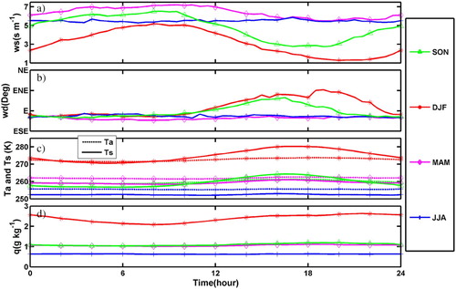
For each season, the data at the same time of a day are averaged and then the seasonal averaged diurnal variation of the meteorological condition can be obtained (Figure 2). It can be seen from Figure 2 that, at Zhongshan station, the meteorological condition showed a remarkable diurnal cycle and also a significant seasonal difference. For the wind speed (Figure 2(a)), the lowest (largest) seasonal mean wind speed 3.2 (6.4) m s⁻¹ occurred in summer (autumn) days, and the largest (smallest) seasonal mean diurnal range 3.9 (0.6) m s⁻¹ was shown in summer (winter). Furthermore, the whole year average was 5.6 m s⁻¹, and the maximum could reach 25 m s⁻¹ (not shown in the figure). For the wind direction (Figure 2(b)), the easterlies prevailed in the whole period. During spring and summer, there was a diurnal variation from easterlies at morning to east–north-easterlies at afternoon, which was related to the land–sea breeze (Xue et al. 2009) and local slope winds caused by the surface heating of solar radiation. For the temperature, annual maximum (minimum) air temperature at 3.9 m height was 280.75 (229.65) K, but maximum (minimum) surface temperature reached 291.05 (230.05) K (not shown in the figure). Seen from Figure 2(c), the seasonal mean diurnal range of temperature at 3.9 m height was very small even during summer (275.55 K), but for surface temperature there was a clear diurnal variation during spring and summer, and the seasonal mean was 280.75, 282.95, 275.75 and 274.05 K for spring, summer, autumn and winter, respectively. During autumn and winter, surface temperature was always lower than the air temperature at 3.9 m height; while during spring and summer, surface temperature was lower (higher) than the air temperature at 3.9 m height at morning (afternoon), showing the diurnal variation of stratification between stable and unstable condition at the surface layer. For the humidity at 3.9 m height (Figure 2(d)), annual mean was 1.2 g/kg (not shown in the figure), and summer (winter) days were the wettest (driest). Compared with other seasons, clearer diurnal variation is shown in summer with a seasonal mean diurnal range of 0.55 g/kg.

Figure 2. Seasonal averaged diurnal variation of (a) wind speed at 3.9 m height, (b) wind direction at 3.9 m height, (c) air temperature at 3.9 m height (solid lines) and radiative temperature of surface (dashed lines), (d) humidity at 3.9 m height collected at the Zhongshan station tower from March 2008 to February 2009.

3.2. Radiation fluxes

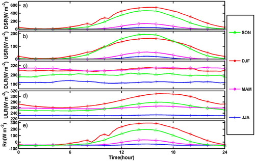
The seasonal averaged diurnal variation of downward shortwave radiation flux (DSR), upward shortwave radiation flux (USR), downward longwave radiation flux (DLR), upward longwave radiation flux (ULR) and net radiation flux (Rn) during the observation period are shown in Figure 3. The annual mean DSR, USR, DLR, ULR and Rn were 115.0, 43.9, 202.0, 258.1 and 15.0 W m⁻², respectively. It can be seen that all the seasonal mean radiation fluxes were the largest in summer and the smallest in winter, which was mainly driven by the seasonal variation of DSR. In summer (winter), seasonal mean DSR, USR, DLR, ULR and Rn were 241.9, 77.6, 210.7, 281.7 and 93.3 (8.0, 4.3, 184.4, 232.1 and −44.0) W m⁻², respectively. Drastically decreasing of DSR from summer to winter made other radiation components reduce significantly (see also Yang et al. 2016 and Yu et al. 2017). Especially, Rn turned from positive values in summer to negative values in winter. Clear seasonal mean diurnal variations were found in DSR and USR (ULR) for all the seasons (spring and summer), but for DLR there was almost no diurnal variation at any a season due to the lack of diurnal variation of the air temperature.

Figure 3. The seasonal averaged diurnal variation of (a) DSR, (b) USR, (c) DLR, (d) ULR and (e) Rn during the period from March 2008 to February 2009 at Zhongshan station.

3.3. Turbulent fluxes

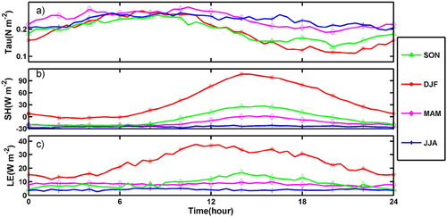
The mean (max) momentum flux τ during this period was 0.22 (3.4) N m⁻², and more than 90% of the time τ was smaller than 0.5 (not shown in the figure). It showed clear diurnal variation during spring, summer and autumn, but not in winter (Figure 4(a)), in consistent with the diurnal variation of wind speed, which also inclined to show the daily maximum (minimum) in the morning (evening). The mean (max) sensible heat flux (SH) during this period was −2.1 (459.3) W m⁻². The negative value means that the ground here absorbs SH from the atmosphere. The SH seasonal averages were −4.4, 40.8, −14.6 and −24.5 W m⁻² during spring, summer, autumn and winter, respectively, Diurnal variation of SH was the most (least) significant in summer (winter) (Figure 4(b)), which was consistent with the variation of surface temperature and DSR. During an average day in summer, most of the time SH was positive, but at night there was still inversion layer which incurred negative SH. In winter, there was strong stable stratification at near surface and SH was always negative. The mean (max) latent heat flux LE during this period was 11.3 (198.1) W m⁻². The LE seasonal averages were 9.1, 24.6, 8.2 and 4.1 W m⁻² during spring, summer, autumn and winter, respectively. It means that during all the seasons vapor was transferred from the ground to atmosphere through sublimation or evaporation. Similar to SH, diurnal variation of LE was the most (least) significant in summer (autumn and winter) (Figure 4(c)).

Figure 4. The seasonal averaged diurnal variation of (a) momentum flux (τ), (b) sensible heat flux (SH) and (c) latent heat flux (LE) during the period from March 2008 to February 2009 at Zhongshan station.

To further investigate the energy distribution, soil heat flux (G) is calculated by(14) $\text{G}=\text{Rn}\text{–}\text{SH}\text{–}\text{LE}\text{–}\text{Re}.$(14) Re is the residual energy involved in various processes, such as photosynthesis, respiration, heat storage and heat away with runoff (Burba, Verma, and Kim 1999). It is assumed Re = 0 here. During autumn (i.e. MAM) and winter (i.e. JJA) Rn, SH and G were all negative, and LE was very small (Figure 5(a)). A negative value of Rn means the surface loses energy through radiation, which is incurred mostly by ULR (Figure 3), and negative values of SH and G indicate that the surface gains energy from the air and the ground which compensate mostly the loss of energy by Rn (Figure 5(a)). During spring, Rn, SH and G were all transiting from negative to positive. During summer, Rn was positive and was consumed by SH, LE and G. The averaged G during the whole period was 6.9 W m⁻², and maximum 82.3 (minimum −25.8) W m⁻² of the seasonal mean was in December (July).

Figure 5. The monthly averaged (a) net radiation flux (Rn), sensible heat flux (SH), latent heat flux (LE) and soil heat flux (G), (b) precipitation, evaporation (or sublimation) and their difference (precipitation minus evaporation) during the period from March 2008 to February 2009 at Zhongshan station.

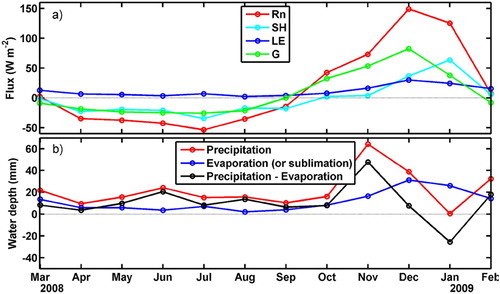
To understand the water balance over this site, the precipitation and evaporation were compared here (Figure 5(b)). The evaporation here is calculated from the latent heat flux from eddy correlation method. It is found that the precipitation during the period was 264.0 mm in total, and it had a seasonal variation with larger (smaller) precipitation around summer (winter) times. The maximum precipitation was in November (64.2 mm), December (38.8 mm) and February (32.3 mm), but a specific low happened in January (0.4 mm), and for the other months precipitation was around 10–20 mm. Generally, precipitation was always larger than evaporation (or sublimation) except in January. For the whole year, the evaporation (or sublimation) was 138.1 mm, and was 125.9 mm smaller than the precipitation.

3.4. Roughness lengths derivation

3.4.1. Aerodynamic roughness length

The aerodynamic roughness length (z₀m) is a parameter that can hardly be determined accurately; it is normally calculated under near-neutral condition (−0.01 ≤ z/L ≤ 0.01) with the following equation:

(15) $z_{0\mathrm{m}}=z/\exp \left(\frac{uk}{u_{\ast }}\right).$(15)

With Equation (15), it can be obtained that(16) $\frac{\mathrm{\Delta }{z}_{0\mathrm{m}}}{z_{0\mathrm{m}}}={\left[\left(\frac{z}{z_{0\mathrm{m}}}\right)\right]}^{\mathrm{\Delta }{u}_{\ast }/u_{\ast }}-1\left(\text{if only considering the error of}{u}_{\ast }\right),$(16) (17) $\frac{\mathrm{\Delta }{z}_{0\mathrm{m}}}{z_{0\mathrm{m}}}={\left[\left(\frac{z_{0\mathrm{m}}}{z}\right)\right]}^{\mathrm{\Delta }u/u}-1\left(\text{if only considering the error of}u\right).$(17) Here, $\mathrm{\Delta }{z}_{0\mathrm{m}},\mathrm{\Delta }{u}_{\ast }$ and $\mathrm{\Delta }u$ are the errors of z₀m, $u_{\ast }$ and $u$, respectively. Equations (16) and (17) show that $u_{\ast }$ (which normally has an error of 10%) leads to about 100% error of z₀m, and $u$ (which normally has an error of 2%) leads to about 10% error of z₀m. Figure 6 shows the calculated log(z/z₀m) from Equations (15) versus wind speed; it is found that z₀m decreases (log(z/z₀m) increases) significantly with an increasing wind speed (u) when u is small (e.g. u ≤ 2 m s⁻¹). Mahrt et al. (2001) proposed that low wind speeds could enhance the viscous effects and reduce the streamlining of surface obstacles, which further resulted in an increase in z₀m when u decreases. However, Zhu and Furst (2013) attributed such z_0m–u relationship to the limitation of MOST, and a varying coefficient was provided to replace the von Kármán constant. Nevertheless, the z_0m – u relationship at u ≤ 2 m s⁻¹ displayed by the data here is not further analyzed, since the observation samples are too few when u ≤ 2 m s⁻¹ (101 dots, 1.7% of the total samples). When u > 2 m s⁻¹, z₀m decreases (log(z/z₀m)) increases) slightly with an increasing wind speed, which is probably related with the footprint of the momentum flux. When the speed of the winds (which are mostly easterlies) is large, a larger proportion of the momentum flux is from the ice sheets west of the site instead of the island (Figure 1(b)), which leads to a smoother averaged underlying surface and smaller z₀m. Based on the measurements, a linear relationship between log(z/z₀m) and u can be defined in 6 m s⁻¹ ≤ u ≤ 12 m s⁻¹ as the black dashed line in Figure 6. For u > 12 m s⁻¹, z₀m decreases (log(z/z₀m) increases) drastically with an increasing wind speed, but due to the small sample size in this region (348 dots, 5.7% of the total samples), such an intensive decrease of z₀m (increase of log(z/z₀m)) may be a mis-presentation and not analyzed here. Besides, a constant z_0m = 3.6 × 10⁻³m (or log(z/z₀m) = 6.93) can be obtained through the overall average as the black solid line in Figure 6. The u_* calculated (u_*cal) under near-neutral condition with the 10-min averaged winds and the two methods of z₀m deduction are compared to the u_* obtained from eddy covariance method (u_*ec), and it shows that there are no significant difference between the two methods (Table 2). In this paper, for the reason of simplicity, the constant z_0m = 3.6 × 10⁻³m is used for further analysis.

Figure 6. The calculated log(z/z₀m) versus wind speed (blue dots), its 0.5 m s⁻¹ bin averaged values (red dots), the partially linear regression (black dashed line) and the overall averaged value (black solid line).

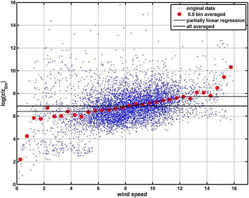
Table 2. The regression slope between u_*cal and u_*ec, and the bias and standard error of u_*cal from u_*ec, for the two methods of z₀m deduction.

The statistics	Partially linear regression	Constant z0m
Regression slope of u*cal – u*ec	0.956	0.978
$\text{Bias}=\sum _{i=1}^n\left|u_{{\ast }_{cal}}-u_{\ast ec}\right|/n$	0.060	0.065
$\text{Normalized standard error ( NSE) }=\sqrt{{\sum }_{i=1}^n{\left|u_{\ast cal}-u_{\ast ec}\right|}^2/{\sum }_{i=1}^n{\left|u_{\ast ec}\right|}^2}$	0.158	0.170

3.4.2. Thermal roughness length

A theoretical model relating the z₀h/z₀m to the surface Reynolds number Re∗ = u∗z₀m/ν was developed by Andreas (1987, hereafter as A87) and modified by Zilitinkevich (1995, hereafter as Z95), Chen, Janjić, and Mitchell (1997, hereafter as C97) and Smeets and Broeke (2008, hereafter as S08), the equations are:(18) $\log \left(\frac{z_{0h}}{z_{0m}}\right)=b_0+b_1[\log ({\text{Re}}_{\ast }\left)\right]+b_2[\log ({\text{Re}}_{\ast }){]}^2$(18) (19) $\log \left(\frac{z_{0\mathrm{h}}}{z_{0\mathrm{m}}}\right)=\frac{1}{kC\sqrt{{\text{Re}}_{\ast }}}.$(19) And for A87, b₀, b₁ and b₂ = 0.317, −0.565 and −0.183 with Equation (18) are applied when 2.5 ≤ Re∗ ≤ 1000, while for S08, b₀, b₁ and b₂ = 1.5, −0.2 and −0.11 with Equation (18) are applied when z_0m ≥ 1 mm_. For Z95 and C97, C = 0.8 and 0.1 are applied with Equation (19), respectively.

With the surface temperature defined as the radiative temperature, the thermal roughness length z₀h can be calculated by Equation (6) through iteration. Vignon et al. (2017) explained that the errors of the calculated z₀h in near-neutral condition are significant because they are proportional to θ_*⁻¹, while in stable or unstable condition the errors are greatly dependent on the choice of the stability functions. Starting from Equation (6), the following equations can be deduced:(20) $\frac{\mathrm{\Delta }{z}_{0\mathrm{h}}}{z_{0\mathrm{h}}}={\left(\frac{z}{z_{0\mathrm{h}}}\right)}^{\mathrm{\Delta }{\theta }_{\ast }/{\theta }_{\ast }}-1(\text{for near}-\text{neutral condition that}\psi \text{is neglected}),$(20) (21) $\frac{\mathrm{\Delta }{z}_{0\mathrm{h}}}{z_{0\mathrm{h}}}=\exp (-\mathrm{\Delta }\psi )-1(\text{for non}-\text{near}-\text{neutral condition and considers only the}\text{error of}\psi ).$(21) Here, $\psi =-{\psi }_H\left(z/L\right)+{\psi }_H\left(z_{0\mathrm{h}}/L\right)$, and $\mathrm{\Delta }{z}_{0\mathrm{h}},\mathrm{\Delta }{\theta }_{\ast }$, and $\mathrm{\Delta }\psi$ are the errors of z₀h, ${\theta }_{\ast }$ and $\psi$, respectively. 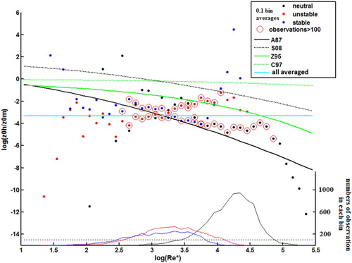Equations (20) and (21) show that, 10% error of ${\theta }_{\ast }$ can lead to about 150% error of z₀h, and 10% error of $\psi$ can lead to about 10% error of z₀h. Therefore, due to the different error sources for different stratifications (i.e. for near-neutral condition, it is mainly from θ_*⁻¹, for stable and unstable conditions the stability functions as the main error sources are different from each other as shown in Equations (8) and (12)), it is noteworthy to compare the calculated z₀h at these different stratification conditions. Figure 7 presents the calculated log(z₀h/z₀m) versus log(Re∗); it is found that the log(z₀h/z₀m) values from the three kinds of stratifications generally agree with each other, especially for the stable and unstable conditions around log(Re∗) = 3, and for neutral and stable conditions around log(Re∗) = 3.8. For the log(Re∗) bin intervals with sample numbers larger than 100, the calculated log(z₀h/z₀m) under the neutral and stable conditions agrees well with A87 equation, while under the unstable condition it generally between A87 and S08. The overall averaged log(z₀h/z₀m) = 3.5, which makes z₀h = 1.2 × 10⁻⁴m.

Figure 7. The calculated log(z₀h/z₀m) versus log(Re∗). The dots are the bin averaged log(z₀h/z₀m) with 0.1 interval of log(Re∗). Observation sample numbers for each stratification condition are shown in the bottom part. Black, red and blue colors represent for neutral, unstable and stable condition, respectively. Red circles indicate that the observation sample number in the bin are larger than 100. A87, S08, Z95, Z97 and a whole averaged z₀h are also shown as black solid, black dashed, green solid, green dashed and cyan solid lines.

With z₀h defined by either of A87, S08, Z95, C97, and the constant value of 1.2 × 10⁻⁴, θ_* can be calculated. The calculated θ_* (θ_*cal) with each of the five methods are compared with the θ_* obtained from eddy covariance method (θ_*ec). Figure 8 shows that all the five methods tend to underestimate θ_* when θ_*ec > 0.2 (which relate to strongly stable stratification), and A87, Z95 and the constant z₀h largely underestimate the absolute value of θ_* when θ_*ec < −0.5 (which relate to strongly unstable condition), while all the five methods generally reproduce θ_* when −0.5 ≤ θ_*ec ≤ 0.2. The statistics of θ_*cal for each z₀h method are shown in Table 3. It can be seen that, when −0.5 ≤ θ_*ec ≤ 0.2, the constant z₀h presents best fit between θ_*cal and θ_*ec, and S08 and C97 overestimate largely the absolute value of θ_*. For the whole range of θ_*ec, the bias and NSE are smallest for A87, and largest for Z97. Because it needs iteration, which also causes self-dependence problem, to obtain the z₀h value for A87, Z95, C97 and S08 methods, the constant value of z₀h = 1.2 × 10⁻⁴m over this site is recommended for its simplicity and also its accuracy especially when −0.5 ≤ θ_*ec ≤ 0.2.

Figure 8. The calculated θ* with (a) A87, (b) S08, (c) Z95, (d) C97 and (e) the constant value of 1.2 × 10⁻⁴ and 10-min averaged wind and temperature observations at 3.7 m height. Blue dots are the original data, and red dots are the 0.05 bin averaged values.

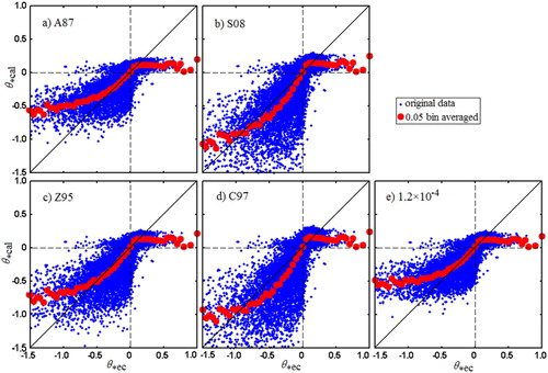
Table 3. The regression slope between θ_*cal and θ_*ec when −0.5 ≤ θ_*ec ≤ 0.2, and the bias and standard error of θ_*cal from θ_*ec, for the five methods of z₀h deduction.

The statistics	A87	S08	Z95	Z97	z0h = 1.2 × 10^−4m
Regression slope of
θ*cal –θ*ec for −0.5 ≤ θ*ec ≤ 0.2	0.912	1.475	1.176	1.580	0.993
Bias	0.078	0.108	0.089	0.119	0.085
Normalized standard error	0.659	0.779	0.673	0.820	0.689

3.5. Validation of the roughness lengths with low frequency observations

The values of z_0m = 3.6 × 10⁻³m and z₀h = 1.2 × 10⁻⁴m are used to calculate u_* and θ_* using the 10 min averaged wind and temperature observations at 2.5, 3.9 and 5.9 m height, and the calculated u_* and θ_* are compared with the values from eddy covariance method (Figure 9 and Table 4). It can be seen that for each height level, the constant roughness lengths’ setting yields reliable u_* and θ_* estimation. The statistics also show that the regression slopes for u_*cal– u_*ec or θ_*cal–θ_*ec (regression of θ_*cal–θ_*ec only carried out in the range of −0.5 ≤ θ_*ec ≤ 0.2) are around 1. The bias (or NSE) of u_* (or θ_*) at three levels are similar to each other, indicating the MOST is mostly applicable at all the three levels. Generally, the θ_{* cal} produces larger bias and NSE than u_*cal. Specially, when θ_*ec < −0.5 or θ_*ec > 0.2, which relate to strongly unstable or stable condition, respectively, the θ_*cal deviates θ_*ec largely, indicating that improvements of θ_* derivation are still needed in these stratifications.

Figure 9. The calculated u_* (upper panels) and θ_* (lower panels) with z_0m = 3.6 × 10⁻³ m and z_0h = 1.2 × 10⁻⁴m and 10-min averaged wind and temperature observations at 2.5, 3.9, and 5.9m height. Blue dots are the original data, and red dots are the 0.05 bin averaged values.

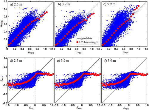
Table 4. The regression slope between u_*cal and u_*ec, or θ_*cal and θ_*ec when −0.5 ≤ θ_*ec ≤ 0.2, and the bias and standard error of u_*cal from u_*ec, or θ_*cal from θ_*ec, with z_0m = 3.6 × 10⁻³ m and z₀h = 1.2 × 10⁻⁴ m and 10-min averaged wind and temperature observations at 2.5, 3.9, and 5.9 m height.

The statistics	u* 2.5 m	u* 3.9 m	u* 5.9 m	θ* 2.5 m	θ* 3.9 m	θ* 5.9 m
Regression slope of u*cal–u*ec or θ*cal–*ec for −0.5 ≤ θ*ec ≤ 0.2	1.087	1.021	1.101	0.923	0.914	0.900
Bias	0.064	0.057	0.068	0.103	0.097	0.096
NSE	0.273	0.239	0.313	0.909	0.905	0.905

4. Summary and conclusions

By using the data observed at Zhongshan station during 3 March 2008 through 15 February 2009, this paper investigates the meteorological condition, radiation and turbulent fluxes characteristics over Zhongshan station, and obtained the aerodynamic and thermal roughness lengths at this site.

Seasonal variations of wind, temperature, humidity, radiation and surface turbulent fluxes were observed. It is found that easterlies dominated this site throughout the whole year, with a maximum (average) speed of 25 (5.6) m s⁻¹ at 3.9 m height, and the annual maximum (minimum) surface temperature reached 291.05 (230.05) K, while the annual maximum (minimum) air humidity was 4.1 (0.05) g/kg at 3.9 m height. The maximum (minimum) values of seasonal mean temperature, humidity, each radiation components, SH and LE were largest in summer (winter), while for seasonal averaged wind speed and τ the minimums (maximums) occurred in summer (autumn). Such a seasonal variation was mostly driven by the enlarged (decreased) DSR in summer (winter), which warmed up (cooled down) the surface and near-surface air, and then increased (decreased) the ULR and air-specific humidity; USR and DLR were also increased (decreased) correspondingly. However, in summer, wind direction was changed more northerly at afternoon due to the development of land–sea breeze and local slope winds as a result of the warm surface and the existence of Larsemann Hills south of Zhongshan station. Besides, smaller wind speed in summer was related to the weakening of the Antarctica katabatic winds (e.g. Parish and Cassano 2001; Nylen, Fountain, and Doran 2004). Diurnal range of wind, temperature, specific humidity, each radiation components and surface fluxes were largest (smallest) in summer (winter). The ground flux was found negative during autumn and winter, and transited to positive in spring and summer. Precipitation was 264.0 mm in total and 125.9 mm of it was left to surface without evaporation or sublimation during the year.

The z₀m is calculated by using the u_* from eddy covariance method, and it is found that z₀m decreases (log(z/z₀m) increases) slightly with an increasing wind speed, which is related with the footprint that covers more smooth ice sheets at larger wind speeds. Partially linear relation is derived between log(z/z₀m) and u, and is compared to the whole averaged z_0m = 3.6 × 10⁻³m. It shows that the u_* calculated from the z₀m by partially linear regression method has smaller bias and NSE, but the regression slope is closer to 1 for the whole averaged z₀m.

The z₀h at different stratification conditions (i.e. neutral, stable and unstable stratification) is also calculated by using the u_* and θ_* from eddy covariance method, and it is found that the log(z₀h/z₀m) values from the three kind of stratifications generally agree with each other when the sample numbers at each bin interval are large, which justifies the reliability of the calculated z₀h because different error source was attached to different stratification condition. An overall average z₀h is found as 1.2 × 10⁻⁴m and was compared to the z₀h equation defined by A87, Z95, C97 and S08. The results show that when −0.5 ≤ θ_*ec ≤ 0.2, the constant z₀h presents best fit between θ_*cal and θ_*ec, while the bias and NSE are smallest for A87.

Overall, considering the reliability and simplicity, and validated by using the other three level observations, z_0m = 3.6 × 10⁻³m and z₀h = 1.2 × 10⁻⁴ m at this site are suggested to be used in future studies. However, the underestimation of the absolute value of θ_* when it is large at strongly stable or unstable condition is significant. Correction for such a bias would need a detailed examination and modification of the MOST, stability functions and roughness length settings, which will be carried out in future studies.

Acknowledgements

We thank the Chinese Arctic and Antarctic Administration and Polar Research Institute of China for the logistic support.

Disclosure statement

No potential conflict of interest was reported by the authors.

Additional information

Funding

This study was supported by the National Natural Science Foundation of China (Grant Nos. 41376005 and 41505004), the National Key Projects of Ministry of Science and Technology of China (2016YFA0602100), the Chinese Polar Environmental Comprehensive Investigation and Assessment Program, and the Open Project Program (KLME1508) of the Key Laboratory of Meteorological Disaster of Ministry of Education at Nanjing University of Information Science and Technology.

References

- Andreas, E. L. 1987. “A Theory for the Scalar Roughness and the Scalar Transfer Coefficients Over Snow and Sea Ice.” Boundary-Layer Meteorology 38 (1): 159–184. doi:10.1007/BF00121562.
- Bian, L. G., L. Y. Lu., and P. Q. Jia. 1997. “Experimental Observation on the Characteristics of the Near-Surface Turbulence Over the Antarctic ice Sheets During the Polar day Period.” Science in China 27 (5): 469–474. doi:10.1360/yd1998-41-3-262.
- Burba, G. G., S. B. Verma, and J. Kim. 1999. “Surface Energy Fluxes of Phragmites Australis in a Prairie Wetland.” Agricultural and Forest Meteorology 94 (1): 31–51. doi:10.1016/S0168-1923(99)00007-6.
- Cassano, John J., T. R. Parish, and J. C. King. 2000. “Evaluation of Turbulent Surface Flux Parameterizations for the Stable Surface Layer Over Halley, Antarctica*.” Monthly Weather Review 129 (1): 26–46. doi:10.1175/15200493(2001)129
- Chen, Fei, Z. Janjić, and K. Mitchell. 1997. “Impact of Atmospheric Surface-Layer Parameterizations in the new Land-Surface Scheme of the NCEP Mesoscale Eta Model.” Boundary-Layer Meteorology 85 (3): 391–421. doi:10.1023/A:1000531001463.
- Cheng, Y. G., and W. Brutsaert. 2005. “Flux-profile Relationships for Wind Speed and Temperature in the Stable Atmospheric Boundary Layer.” Boundary-Layer Meteorology 114 (3): 519–538. doi:10.1007/s10546-004-1425-4.
- Gillett, N. P., and D. W. Thompson. 2003. “Simulation of Recent Southern Hemisphere Climate Change.” Sciences 302 (5643): 273–275. doi:10.1126/science.1087440.
- Guo, Zhichang, D. H. Bromwich, and J. J. Cassano. 2002. “Evaluation of Polar MM5 Simulations of Antarctic Atmospheric Circulation*.” Monthly Weather Review 131 (2): 384–411. doi:10.1175/1520-0493(2003)131
- Hendon, H. H., D. W. J. Thompson, and M. C. Wheeler. 2007. “Australian Rainfall and Surface Temperature Variations Associated with the Southern Hemisphere Annular Mode.” Journal of Climate 20 (11): 2452–2467. doi:10.1175/JCLI4134.1.
- King, J. C., W. M. Connolley, and S. H. Derbyshire. 2001. “Sensitivity of Modelled Antarctic Climate to Surface and Boundary-Layer Flux Parametrizations.” Quarterly Journal of the Royal Meteorological Society 127 (573): 779–794. doi:10.1002/qj.49712757304.
- Li, S. M., X. Q. Wang., M. Y. Zhou., F. Xue., B. R. Li., and S. D. Wang. 2010. “A Polar Regions Flux Observation System and its Application in the IPY Global Coordinated Observation.” Marine Forecasts 27 (1): 62–71.
- Lin, Z., L. G. Bian, Y. F. Ma, and C. G. Lu. 2009. “Turbulent Parameters of the Near Surface Layer Over the ice Sheet Nearby Zhongshan Station, East Antarctica.” Chinese Journal of Polar Research 21 (3): 221–233.
- Mahrt, L., Vickers Dean, Sun Jielun, Jensen Niels Otto, Jørgensen Hans, Pardyjak Eric, and Fernando Harindra 2001. “Determination of the Surface Drag Coefficient.” Boundary-Layer Meteorology 99 (2): 249–276. doi:10.1023/A:1018915228170.
- Moncrieff, J., R. Clement, J. Finnigan, and Meyers, T. 2005. “Averaging, Detrending, and Filtering of Eddy Covariance Time Series.” Handbook of Micrometeorology 29: 7–31. doi: 10.1007/1-4020-2265-4_2
- Nylen, Thomas H., A. G. Fountain, and P. T. Doran. 2004. “Climatology of Katabatic Winds in the McMurdo dry Valleys, Southern Victoria Land, Antarctica.” Journal of Geophysical Research Atmospheres 109 (3): 323–350. doi:10.1029/2003JD003937.
- Parish, Thomas R, and J. J. Cassano. 2001. “The Role of Katabatic Winds on the Antarctic Surface Wind Regime.” Monthly Weather Review 131 (131): 317–333. doi:10.1175/1520-0493(2003)131.
- Paulson, C. A. 1970. “The Mathematical Representation of Wind Speed and Temperature in the Unstable Atmospheric Surface Layer.” Journal of Applied Meteorology 9 (9): 857–861. doi:10.1175/1520-0450(1970)009
- Qu, S. H., and D. Y. Gao. 1996. “Characteristics of Atmospheric Boundary Layer Structure and Transfer of the Turbulent Fluxes Over the Zhongshan Station Area, Antarctica.” Chinese Journal of Polar Research 8 (4): 2–10.
- Reijmer, C. H, E. V. Meijgaard, and M. R. V. D. Broeke. 2003. “Roughness Length for Momentum and Heat Over Antarctica in a Regional Atmospheric Climate Model.” In Proceedings of the seventh conference on polar meteorology and oceanography and joint symposium on high-latitude climate variations, Hyannis, Massachusetts. Washington, DC, American Meteorological Society. CD-ROM, May 12–16.
- Schneider, D. P., E. J. Steig, and J. C. Comiso. 2004. “Recent Climate Variability in Antarctica From Satellite-Derived Temperature Data.” Journal of Climate 17 (7): 1569–1583. doi:10.1175/1520-0442(2004)017
- Smeets, C. J. P. P., and M. R. V. D. Broeke. 2008. “The Parameterisation of Scalar Transfer Over Rough Ice.” Boundary-Layer Meteorology 128 (3): 339–355. doi:10.1007/s10546-008-9292-z.
- Vignon, E., Genthon, C., Barral, H., Amory, C., Picard, G., & Gallée, H., Casasanta Giampietro, Argentini Stefania. 2017. “Momentum- and Heat-Flux Parametrization at Dome C, Antarctica: A Sensitivity Study.” Boundary-Layer Meteorology 162: 341–367. doi:10.1007/s10546-016-0192-3.
- Webb, E. K., G. I. Pearman, and R. Leuning. 1980. “Correction of Flux Measurements for Density Effects due to Heat and Water Vapour Transfer.” Quarterly Journal of the Royal Meteorological Society 106 (447): 85–100. doi:10.1002/qj.49710644707.
- Xue, F., Z. Zhang, M. Zhou, S. Li, B. Li, and B. Sun. 2009. Characteristics of the Surface Wind in Summer at the Continental Margin, East Antarctica. Chinese Journal of Polar Research 21 (4): 288–298.
- Yang Q., J. Liu, M. Lepparanta, Q. Sun, R. Li, L. Zhang, T. Jung, et al. 2016. “Albedo of Coastal Landfast sea ice in the Prydz Bay, Antarctica: Observations and Parameterization.” Advances in Atmospheric Sciences 33 (5): 535–543. doi:10.1007/s00376-015-5114-7.
- Yu, L., Q. Yang, M. Zhou, D. H. Lenschow, X. Wang, J. Zhao, Q. Sun, Z. Tian, H. Shen, L. Zhang. 2017. “The Variability of Surface Radiation Fluxes Over Landfast sea ice Near Zhongshan Station, East Antarctica During Austral Spring.” International Journal of Digital Earth in Press 120: 1–18 doi:10.1080/17538947.2017.1304458.
- Zhu, P., and J. Furst. 2013. “On the Parameterization of Surface Momentum Transport via Drag Coefficient in low-Wind Conditions.” Geophysical Research Letters 40 (11): 2824–2828. doi:10.1002/grl.50518.
- Zilitinkevich, S. S. 1995. “ Non-Local Turbulent Transport: Pollution Dispersion Aspects of Coherent Structure of Convective Flows.” Air Pollution Theory and Simulation, Computational Mechanics Publications, Southampton, Boston, pp. 53–60.