Quantifying individual tree growth and tree competition using bi-temporal airborne laser scanning data: a case study in the Sierra Nevada Mountains, California

ABSTRACT

Improved monitoring and understanding of tree growth and its responses to controlling factors are important for tree growth modeling. Airborne Laser Scanning (ALS) can be used to enhance the efficiency and accuracy of large-scale forest surveys in delineating three-dimensional forest structures and under-canopy terrains. This study proposed an ALS-based framework to quantify tree growth and competition. Bi-temporal ALS data were used to quantify tree growth in height (ΔH), crown area (ΔA), crown volume (ΔV), and tree competition for 114,000 individual trees in two conifer-dominant Sierra Nevada forests. We analyzed the correlations between tree growth attributes and controlling factors (i.e. tree sizes, competition, forest structure, and topographic parameters) at multiple levels. At the individual tree level, ΔH had no consistent correlations with controlling factors, ΔA and ΔV were positively related to original tree sizes (R > 0.3) and negatively related to competition indices (R < −0.3). At the forest-stand level, ΔH and ΔA were highly correlated to topographic wetness index (|R| > 0.7), ΔV was positively related to original tree sizes (|R| > 0.8). Multivariate regression models were simulated at individual tree level for ΔH, ΔA, and ΔV with the R² ranged from 0.1 to 0.43. The ALS-based tree height estimation and growth analysis results were consistent with field measurements.

KEYWORDS:

• Airborne Laser Scanning
• change detection
• tree growth
• tree competition
• Sierra Nevada

1. Introduction

The Sierra Nevada (SN) mountain range, covering an area of 63,100 km², is the home to one of the most diverse temperate conifer forests on Earth (Battles et al. 2001; Britting et al. 2012). The SN forests provide California with many forest services, including wildlife habitats, carbon stocks, water provision, and economic and cultural values (Bales et al. 2011). Spatially explicit and efficient quantification and modeling of tree growth are critical for SN forests resource evaluation, management, and protection (Battles et al. 2008).

Forest growth models, such as the California Conifer Timber Output Simulator (CACTOS) and the climate adjustment of CACTOS, have been developed either to simulate short-term timber yield (Wensel, Meerschaert, and Biging 1987) or to project tree growth under a changing climate (Battles et al. 2008) at individual tree to landscape scales (Battles et al. 2006, 2008; Biging and Wensel 1984; Weiskittel et al. 2011; Wensel, Meerschaert, and Biging 1987). Tree growth models, particularly at the individual tree level, relied heavily on forest inventory data (Biging and Wensel 1984; Tompalski et al. 2016; Weiskittel et al. 2011; Wensel, Meerschaert, and Biging 1987). However, taking in-situ measurements is often time-consuming and labor-intensive. Traditional models mainly focused on the growth in tree height and/or diameter at breast height (DBH) (Pretsch 2009; Weiskittel et al. 2011). Tree crown expansion, which is an essential part of tree growth in terms of light interception, gas exchange, and water transpiration (Hardiman et al. 2013), has been rarely studied due to difficulties in obtaining direct field measurements (Weiskittel et al. 2011). Moreover, competition indices, which quantify competition among trees for resources, are important inputs in many tree growth models. The estimation of crown size for competition indices calculation were often based on indirect regression from tree height and DBH, which might be fraught with uncertainty issues (Biging and Dobbertin 1995; Wensel, Meerschaert, and Biging 1987). Therefore, accurate and efficient estimation of tree growth and tree competition at various scales has become an issue needed to be addressed for precise forest growth modeling and management (Olivier, Robert, and Fournier 2016).

Airborne Laser Scanner (ALS) data are playing an increasingly important role in forest survey (Jakubowski et al. 2013; Korhonen et al. 2011; Latifi et al. 2012; Su, Ma, and Guo 2016; Tompalski et al. 2016) because of their capabilities in characterizing three-dimensional tree structures at forest-stand (Coops et al. 2007; Hyyppä et al. 2008; Næsset and Økland 2002; Su, Guo, Fry, et al. 2016; Tao et al. 2014; Tempel et al. 2015) and individual tree levels (Li et al. 2012; Lu et al. 2014; Zhen, Quackenbush, and Zhang 2016). Many studies have demonstrated the efficiency and accuracy of using ALS data to estimate forest structure parameters, including tree height (Breidenbach et al. 2008; Dubayah et al. 2010; Holmgren, Nilsson, and Olsson 2003; Yu et al. 2006), crown base height (CBH) (Holmgren and Persson 2004; Popescu and Zhao 2008), crown area (Casas et al. 2016; Gonzalez-Benecke et al. 2014), crown volume (Kato et al. 2009), stem volume (Chen et al. 2007), canopy cover (CC) (Korhonen et al. 2011; Moeser et al. 2014), aboveground biomass (Cao et al. 2016; Singh et al. 2015; Singh et al. 2017; Tao et al. 2014), and basal area (Véga et al. 2016). Furthermore, ALS data have advantages over traditional in-situ measurements in estimating forest competition efficiently over large areas (Lo and Lin 2013; Pedersen et al. 2012).

Recently, techniques have been developed to detect tree growth from multi-temporal ALS data. At the forest-stand level, Yu et al. (2008) quantified mean tree height and volume growth in a boreal forest using multi-temporal ALS data; and Dubayah et al. (2010) estimated forest height and biomass dynamics in tropical forests. At the individual tree level, several researchers have successfully used multi-temporal ALS data to detect tree height growth (Londo 2010; Song et al. 2016), canopy height growth (Yu et al. 2006), and crown growth (Frew et al. 2016). Moreover, studies have been increased on analyzing the relationships between tree growth and its controlling factors using multi-temporal ALS data. For example, Vepakomma, St-Onge, and Kneeshaw (2011) assessed the responses of tree growth to canopy openings in a boreal forest. However, most previous studies either estimated a single attribute of tree growth rather than multi-attributes (Londo 2010), or they focused on how tree growth was impacted by a single group of factors, such as competition index (Olivier, Robert, and Fournier 2016) and topographic condition (Adams, Barnard, and Loomis 2014). A comprehensive study is needed to systematically analyze how different factors influence tree growth in multi-attributes at various scales.

This study aimed to quantify tree growth and analyze its controlling factors in the SN forests using bi-temporal ALS data. Three specific research questions were addressed. (1) How to quantify tree growth in height, crown area, and crown volume at individual tree and forest-stand scales from bi-temporal ALS data? (2) How to estimate tree competition indices from ALS data? (3) How does tree growth respond to various impact factors at different scales? Knowledge obtained in this study can provide guidance for tree growth modeling and forest management in SN forests.

2. Materials

2.1. Study area

Our study areas, Last Chance (39° 07′ N, 120° 36′ W) and Sugar Pine (37° 25′ N, 119° 36′ W), are in the northern and southern SN mountain ranges (Figure 1). The elevation ranges from 730 m to 2190 m in Last Chance and from 730 m to 2650 m in Sugar Pine. Both areas have a Mediterranean climate. The annual total precipitation during the study period in Last Chance (2008–2013) was 1661 mm on average with a range from 255 mm to 2500 mm, and in Sugar Pine (2007–2012) was 1106 mm on average with a range from 589 mm to 1839 mm. Coniferous trees are the dominant species in both areas. In last chance, white fir (WFR) (Abies concolor) and red fir (RFR) (Pseudotsuga menziesii) are two most abundant species, followed by incense cedar (Calocedrus decurrens), sugar pine (Pinus lambertiana), ponderosa pine (PPN) (Pinus ponderosa), and California black oak (Quercus kelloggii). Trees in Sugar Pine had similar species composition but slightly different species abundance.

Figure 1. The geolocation of the last chance and sugar pine study areas and the distribution of 17 selected study sites and 61 field-measured plots.

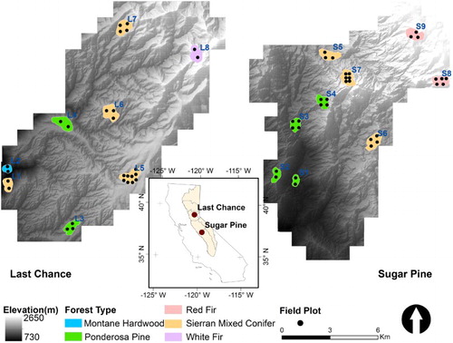
Initially, we selected 25 study sites, which covered a range of forests with different dominant tree species, canopy densities, and topographic conditions (Figure S1). The selection of different forest types was guided by the vegetation map from the Classification and Assessment with Landsat of Visible Ecological Groupings system (CALVEG) (Franklin, Woodcock, and Warbington 2000). Originally, there were two Montane Hardwood (MHW), eight PPN, nine Sierran Mixed Conifer (SMC), four RFR, and two WFR forest sites selected from the CALVEG data (Figure S1(a)). The 25 sites were evenly distributed over the elevation zones from 900 m to 2500 m (Figure S1(b)). Since we mainly focused on the tree growth under natural conditions, study sites with observable disturbances, such as forest fires and treatments, were excluded. The disturbed areas were detected by calculating the stand-level average CC differences between two sets of ALS data (Su, Guo, Collins, et al. 2016). Finally, 17 sites were chosen for this study (Figure S1(c)), which included 1 MHW, 6 PPN, 7 SMC, 2 RFR, and 1 WFR forest stands (Figure 1). We manually delineated boundaries for each study site following two criteria: (1) each site should belong to the same forest type defined by CALVEG; and (2) each site should contain more than 4000 trees to guarantee enough samples for correlation analysis. Thus, the final study sites had different sizes, varied from 0.22 km² to 0.55 km². The site mean tree height ranged from 9.4 m to 31.2 m and the CC varied from 38% to 97% (Table S1).

2.2. Field measurements

We obtained 61 in-situ plot measurements (∼500 m² in a circle for each plot) in the study sites to validate ALS-based tree height and growth results (Figure 1). These measurements were taken in the summers of 2007 and 2008 and re-measured in 2012 and 2013. Plot center locations were measured using a Trimble™ GeoXH GPS. Within each plot, all live trees with a DBH larger than 5 cm were tagged for the repeated surveys. The tree vigor conditions for both surveys were recorded following the forest inventory and analysis standard (Schomaker et al. 2007). In total, 560 trees from six different species were measured, including 327 PPN, 76 WFR, 103 RFR, 15 ICD, 23 SPN, and 16 CBO (Table S2). The species and tree height information were used in the tree height growth analysis.

2.3. ALS data and pre-processing

Bi-temporal small footprint ALS data were acquired using the same scanner unit, the Optech GEMINI airborne laser terrain mapper (ALTM) system, in September 2008 and August 2013 for Last Chance, and in September 2007 and November 2012 for Sugar Pine. The ALS data were collected at 600–800 m above the ground, with a 67% swath overlap on average. The ALTM sensor was operated at 100 kHz with a scanning frequency of 40–60 Hz and a scan angle of 12–14° on either side of nadir. Up to four discrete returns were collected per shot. The delivered data had an averaged density of 10 points/m². To guarantee that the bi-temporal ALS flights could be aligned, we selected over 800 ground checkpoints using ground GPS to calibrate the ALS data both vertically and horizontally. The obtained spatial accuracy was around 10 cm horizontally and 5–35 cm vertically. Note that the 2007/2008 ALS data and 2012/2013 ALS data are referred as ALS1 and ALS2 hereafter.

The digital terrain model (DTM), digital surface model (DSM), and canopy height model (CHM) were the three basic ALS-derived metrics used to generate three tree growth metrics (i.e. tree height, crown area, and crown volume) and four sets of factors (i.e. original tree size, competition indices, forest structures, and topographic conditions) for this study. The DTM and DSM for each study period were interpolated from ALS ground returns and first returns using the ordinary Kriging algorithm, respectively (Guo et al. 2010). CHM was calculated as the difference between the DSM and DTM. We chose 0.5 m as the resolution for DTM, DSM, and CHM because it was a balance between accuracy and computational efficiency, and it was used in a similar study (Tao et al. 2014).

3. Methodology

The methodology for tree growth detection and analysis in tree height (ΔH), crown area (ΔA), and crown volume (ΔV) is shown in Figure 2 and introduced in the following sections.

Figure 2. Flowchart of the methodology. ΔH, ΔA, and ΔV mean tree height, crown area, and crown volume.

3.1. Tree growth detection

3.1.1. Individual tree segmentation

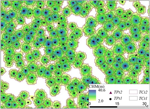
We used the Marker-controlled Watershed Segmentation (MWS) algorithm to delineate individual tree crowns from all ALS-derived CHMs. MWS is a well-known image segmentation algorithm, which combined advantages in region-growing and edge-detection algorithms (Meyer and Beucher 1990). MWS has been successfully applied to segment individual tree crowns from ALS data in many studies (Chen et al. 2006; Tao et al. 2014). Before the segmentation, we applied the Gaussian filter with two times the standard deviation to suppress irrelevant local maxima and fill pits in CHM (Chen et al. 2006). Based on field surveys, a 2-m threshold was selected to separate shrubs from trees. The MWS segmentation was conducted with a 3 × 3 moving window in the System for Automated Geoscientific Analyses (SAGA) software (Tao et al. 2014). To refine results from auto-segmentation, we deleted small segments (area <1 m²), and manually redrew extremely large-area (area >150 m²) or elongate-shape (shape index >4) (Li et al. 2012) segments through visual interpretation of CHM (Figure 3).

Figure 3. An example of tree crown segmentation results and the corresponding tree top locations. TPt1/2 are tree tops and TCt1/2 are tree crowns detected from ALS1/2, respectively.

3.1.2. Tree size metrics estimation

Three tree size metrics (i.e. tree height, crown area and crown volume) were estimated from the ALS data, because they are important indicators of tree vigor and competitiveness for natural resources (Burkhart and Tomé 2012). Each individual tree height was calculated as the maximum CHM value within its segmented tree crown, and tree crown area was represented by the area of each segment. The tree crown volume is usually defined as the volume between the CHM and CBH, and many methods have been developed to quantify them from ALS data (Kato et al. 2009; Popescu and Zhao 2008; Vauhkonen et al. 2008, 2009). In this study, we approximated the crown volume by calculating the volume above the minimum CHM value within each segment (Tao et al. 2014). The minimum CHM value was used as a proxy of CBH, and the sum of CHM values above the CBH in each segment was multiplied by the pixel unit area (0.25 m²) to estimate the crown volume.

3.1.3. Estimation of individual tree growth

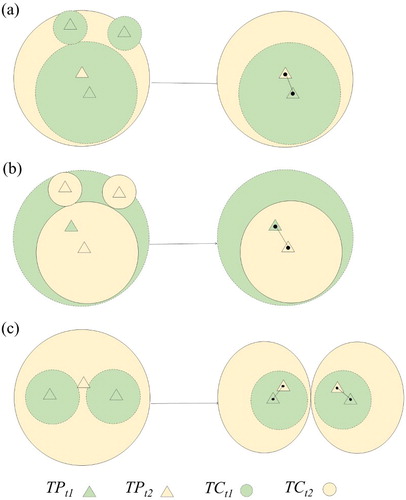
Individual tree growth was estimated as the changes in tree size metrics estimated from ALS1 to ALS2. Precisely pairing up individual trees from ALS1 and ALS2 was a crucial step for accurate tree growth detection. In this study, each tree pair from ALS1 and ALS2 was recognized as the same tree only if the following two criteria were met simultaneously: (1) tree top from ALS1/ALS2 was the only tree top located in the tree crown from ALS2/ALS1; (2) the distance between the tree tops from ALS1 and ALS2 was less than 2 m. The second criterion was set to compensate for the mismatch of tree tops caused by ALS mis-registration. As shown in Figure 4, there were three scenarios that might fail to meet the above-mentioned criteria and needed manual pairing. Scenarios 1 and 2 represented conditions where small trees disappeared/appeared in ALS2 (Figure 4(a,b)). For these two scenarios, we manually removed small trees that disappeared/appeared and paired the two trees sharing the largest tree crown. Scenario 3 represented the condition that one tree top in ALS1 was mis-detected in ALS2 (Figure 4(c)). To pair these tree tops, we manually split the detected tree top in ALS2 into two tree tops by visual examination, and re-performed the tree segmentation to derive new ALS2 tree crowns. Besides, there were rare cases where the ASL1 and ALS2 tree tops satisfied the first rule, but were more than 2 m away from each other. We treated this situation as segmentation errors, and deleted them from tree segmentation results.

Figure 4. A schematic figure showing manual editing on tree pairing under three scenarios: (a) the crown area of the dominant tree increased from ALS1 to ALS2; (b) the crown area of the dominant tree decreased from ALS1 to ALS2; and (c) tree crowns were mis-segmented in ALS2. TPt1/2 are tree tops and TCt1/2 are tree crowns detected from ALS1/2, respectively.

3.2. Calculation of tree growth factors

In this study, four sets of widely used tree growth modeling factors were calculated from ALS1, namely the original tree sizes, topographic parameters, competition indices, and forest structure indices (Adams, Barnard, and Loomis 2014; Biging and Dobbertin 1995; Das 2012; Goulden et al. 2016; Twery and Weiskittel 2013). The original tree sizes were derived using the above-mentioned tree growth detection procedure. The methods for calculating the other three sets of factors are described below.

3.2.1. Topographic parameters

Variations in topographic conditions can result in different solar and water resource distributions, and consequently influence tree growth (Adams, Barnard, and Loomis 2014). In this study, we calculated four topographic parameters including elevation, slope, global insolation (GI), and topographic wetness index (TWI) from ALS1-derived DTM. GI indicates topographically determined potential solar resources, and is defined as the sum of direct and diffused solar radiance per unit area in a year (Rich et al. 1994). In this study, slope and GI were calculated using the ESRI™ ArcMap software. TWI describes the probability of an area being saturated based on its catchment area and slope (Moore, Grayson, and Ladson 1991), and it quantifies topographic determined soil moisture and water availability, which has been a major restriction of tree growth in the SN forests (Trujillo et al. 2012). In this study, TWI was calculated using SAGA software. Since the variations of these parameters within each site were small, we used the site mean values to analyze their impacts on site-level tree growth (Figure 2).

3.2.2. Competition indices

Competition indices are designed to quantify competition among trees for resources in tree growth modeling (Biging and Dobbertin 1995; Twery and Weiskittel 2013; Wensel, Meerschaert, and Biging 1987). Generally, competition indices can be divided into three categories: distance-dependent indices, distance-independent indices, and semi-distance-independent indices. Distance-dependent indices quantify fine-scale variation in competition by considering the distance from a tree to its neighbors, whereas distance-independent indices neglect the distance and treat every tree equally. Semi-distance-independent indices compromise the precision in distance-dependent indices and the efficiency in distance-independent indices (Contreras, Affleck, and Chung 2011), and thus have advantages in large-area applications. In this study, we calculated four semi-distance-independent indices from ALS1 data, including tree number (TN), crown competition of all tree crowns (CCT), crown competition of 66% tree height (CC66), and crown competition of higher trees (CCHT).

TN is the number of trees in a subject tree’s neighborhood (Reineke 1933). CCT, CC66 and CCHT are three crown-based indices, which quantify the percentages of competitive crown areas in a subject tree’s neighborhood under different definitions of competitive crown areas (Biging and Dobbertin 1995). As shown in Equations (1)–(3), CCT counts the percentage of all tree crowns (CHM >2 m) (Biging and Wensel 1990), CC66 counts the percentage of tree crowns taller than 66% of the subject tree (Krumland 1982), and CCHT counts the percentage of tree crowns taller the subject tree (Biging and Dobbertin 1995). The competition indices were calculated using R language (RCore 2013) programming based on Equations (1)–(3), from individual tree crown and tree top segmentation results and CHM data.(1) (2) (3)

where is the area of the defined neighborhood, which is a circle with 15 m radius centered by the subject tree top in this study, is the crown area of a subject tree, and is the height of a subject tree. To avoid the edge effect, trees crowns within 15 m of site boundaries were excluded from the competition indices calculation.

3.2.3. Forest structure indices

We selected three forest structure indices including CC, density of tree (DT), and average nearest neighbor index (NNI) to quantify site-level tree competition. We calculated CC as the percentage of pixels with CHM higher than 2 m in each site. DT was defined as the total number of trees segmented from ALS data divided by the area of each site. NNI was the average distance of each tree to the nearest tree in a site divided by the average distance from a hypothetical random distribution. A site with a NNI smaller than one has a clustering tree distribution pattern, whereas the site with a NNI greater than one has a dispersed pattern (David 1985).

3.3. Correlation analysis and multivariate regression model

We assessed the correlations between tree growth and its controlling factors using the Pearson’s correlation coefficient (R). A natural-logarithm was applied on tree size and tree growth parameters to transform their distributions into normal ones. We also estimated the correlations among all impact factors to show the multicollinearity. Finally, we built multivariate linear regression models for tree growth in ΔH, ΔA, and ΔV from variables with substantial correlations to them. The stepwise variable selection based on the Akaike’s information criterion (Akaike 1974) method was applied to refine the model generation using the stepAIC function in R MASS package (Ripley 2002).

3.4. Accuracy assessment

Field-measured tree height was used to validate the ALS-based tree height estimation and growth analysis results. The tree height validation was conducted at the plot level, since the individual tree location was not available from the field in this study. We calculated the mean value of ALS-based tree height estimates in each plot, and compared them with field-measured plot mean tree height. The root-mean-square-error (RMSE) and bias were used to assess the accuracy of ALS-based estimations. Field-measured plot mean tree height growth (ΔfH) and its correlations to original plot mean tree height (fH1) and topographic parameters were also calculated to verify the correlations from ALS estimation. At the individual tree level, the correlation between ΔfH and fH1 was analyzed by species, instead of by site because there were only 33 trees measured in each site on average. As individual tree locations and crown sizes were not measured from the field, this study only provided a partial assessment of ALS-derived results.

4. Results

4.1. Tree growth detection

There were 53,338 and 61,293 trees segmented and matched from bi-temporal ALS data in Last Chance and Sugar Pine, respectively. The mean value of tree height, crown area, and crown volume from ALS1 was 15.6 m, 18.5 m², and 189.3 m³ in Last Chance, and 15.9 m, 26.5 m², and 198.5 m³ in Sugar Pine (Figure 5).

Figure 5. Distributions of tree height, crown area, and crown volume at (a) Last Chance and (b) Sugar Pine from ALS1 and ALS2. The mean values of the changes from ALS1 to ALS2 are also labeled for each site.

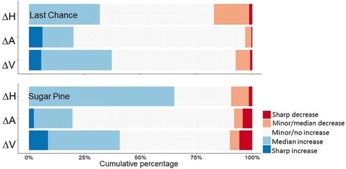
On average, tree size increased on both areas, larger increase in tree crown area and volume was observed in Last Chance, and more tree height growth in Sugar Pine (Figure 5). More specifically, we categorized these changes into five classes (Figure 6). Most trees (83–97%) experienced increases in their sizes, and 1–6% experienced a sharp increase. Trees in Sugar Pine showed 7% more growth in tree height than in Last Chance, whereas trees in Last Chance showed 3–5% more crown expansions.

Figure 6. Comparison of the cumulative proportions of tree size changes from ALS1 to ALS2 in Last Chance and Sugar Pine in five classes: sharp increase (ΔH ≥ 10 m, ΔA ≥ 20 m2, and ΔV ≥ 200 m3), median increase (1 m ≤ ΔH < 10 m, 10 m2 ≤ ΔA < 20 m2, and 50 m3 ≤ ΔV < 200 m3), minor/no increase (0 m ≤ ΔH < 1 m, 0 m2 ≤ ΔA < 10 m2, and 0 m3 ≤ ΔV < 50 m3), minor/median decrease (−10 m ≤ ΔH < 0 m, −20 m2 ≤ ΔA < 0 m2, and −200 m3 ≤ ΔV < 0 m3), and sharp decrease (ΔH < −10 m, ΔA < −20 m2, and ΔV < −200 m3).

The mean and standard deviation of tree sizes for each study site differed substantially (Figure 7). Among the 17 sites, L3 and S2 sites were young PPN forest stands with small variations in size. The SMC sites in L1, S5, and S6 had relatively large mean values and standard deviations.

Figure 7. Comparisons of (a) tree height, (b) crown area, and (c) crown volume among 17 study sites. Black and grey bars are the mean values of tree sizes estimated from ALS1 and ALS2. Error bars show one standard deviation of tree sizes in each site.

4.2. Individual tree level tree growth responses to controlling factors

Correlations between tree growth in height and controlling factors were relatively weak (Figure 8(a)). The maximum absolute R (|R|) was lower than 0.4 among all sites, albeit most of them were significant. Factors with the strongest correlation changed from site to site. In general, H1 was the most influential factor to ΔH in 8 out of 17 sites. Competition indices could be either negatively or positively correlated with ΔH among different study sites and indices.

Figure 8. Correlation coefficients between tree growth in (a) height, (b) crown area, and (c) crown volume and original tree size (H1, A1 and V1) and competition indices (CCT, CC66, CCHT, and TN).

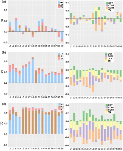
The correlations between tree crown area growth and controlling factors were stronger and more consistent than those with tree height growth (Figure 8(b)). A1 had the strongest positive correlations with ΔA in most sites (averaged R: 0.41), followed by V1 (averaged R: 0.39) and H1 (averaged R: 0.32). CC66 and CCHT were the most influential competition indices, which were negatively correlated with ΔA. On average, the |R| with ΔA for CC66 (0.31) and CCHT (0.31) were 505% and 93% higher than that for the CCT and TN, respectively.

As expected, tree growth in crown volume was positively related with original tree sizes, and negatively impacted by competition indices, but the correlations were stronger than those in crown area (Figure 8(c)). The average |R| in ΔV was approximately 53% higher than ΔA, and 308% higher than ΔH. ΔV had the strongest correlation with V1 (R: 0.48 to 0.76), and CCHT is the most influential competition indices on ΔV among most sites (R: −0.39 to −0.59).

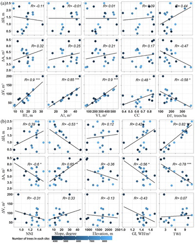
4.3. Site-level tree growth responses to controlling factors

Site-level tree height growth had the strongest correlation with TWI (R = 0.82), followed by Slope (R = −0.53), but no significant correlation with other factors. Site mean crown area growth had the strongest correlation with TWI (R = −0.78), followed by slope (R = 0.65) and NNI (R = −0.6), but no significant correlation with original tree sizes. Site mean crown volume growth, on the contrary, was strongly controlled by the original tree sizes (0.85 ≤ R ≤ 0.9), but had no correlation with topographic parameters (Figure 9).

Figure 9. Scatter plots between site-level tree growth in ΔH, ΔA, ΔV and 10 factors from original tree sizes (H1, A1, and V1); forest structure indices (CC, DT, and NNI); and topographic parameters (slope, elevation, GI, and TWI). Each dot presents a site mean value and its color indicates the number of trees in each site. The regression line is presented in the black line. R is labeled as significant at the confidence level of 99.9% (***), 99% (**), and 95% (*).

4.4. Multivariate regression modeling of tree growth

Multivariate linear regressions for individual tree growth in height, crown area, and crown volume from original tree sizes, competitions, and site-level impact factors are shown in Equations (4)–(6). Variables in the models were selected from those with significant correlations with tree growth (Figures 8 and 9). We also filtered out the variables with strong multicollinearity based on the correlation matrix among all factors (Figure S2). All variables were normalized using their mean and standardize deviation to reduce the scale effects before regression. The coefficients of determination (R²) for these models were 0.24 for ΔH, 0.10 for ΔA, and 0.43 for ΔV, and they were significant at the confidence level of 99.9%. The RMSE and relative RMSE of predicted ΔH, ΔA, and ΔV were 0.94 m (53.9%), 4.87 m² (77.9%), and 51.99 m³ (63.2%), respectively.(4) (5) (6)

4.5. Validation using tree height field measurements

Mean tree height in all the 61 plots from two ALS estimates was validated using field measurements (Figure 10). The R² between ALS estimation and field measurements were both 0.96, the RMSE were 0.82 m and 0.85 m from the data collected in the first- and second-time periods, respectively. The field-measured tree heights were slightly higher (0.63 m and 0.11 m on average) than values from ALS estimation. Overall, the ALS-based tree height was consistent to tree height measured in the field.

Figure 10. Comparison between ALS estimated tree height and field-measured tree height at plot level. Subfigure (a) and (b) show data collected in the first and second-time periods over 61 plots.

At the individual tree level, correlations between field-measured tree height growth (ΔfH) and original tree height (fH1) were positive for PPN (R = 0.27); but negative for RFR (R = −0.32) and WFR (R = −0.21) species. No significant correlation was found when combining all species. At the plot level, the ΔfH had the strongest correlation with TWI (R = 0.51), and was also responsive to fH1 with a lower correlation (R = 0.27). No significant relationship was found between ΔfH and any other environmental parameters. These results were consistent with the correlations observed from ALS-based estimates.

5. Discussion

Previous studies have found that individual tree growth was positively determined by internal tree competitiveness, such as original tree sizes, and negatively influenced by external tree competition, owing to limited solar and water resources (Aakala et al. 2013; Biging and Dobbertin 1995; Weiskittel et al. 2011; Wensel, Meerschaert, and Biging 1987). Our results generally agreed with these arguments, but the correlations between impact factors and tree growths in ΔH, ΔA, and ΔV varied by factors and sites.

ΔV had a stronger correlation with the original tree sizes than ΔA and ΔH (Figure 8). Ideally, absolute crown growth of a vigorous tree should be proportional to its original crown size if the same amount of elongation occurs in the main stem and branches (Pretzsch 2014; Weiskittel et al. 2011). However, the horizontal elongation of a tree crown, quantified by ΔA in this study, was also constrained by the space availability between trees, and thus was less linearly related to the original size than ΔV. Studies have shown that ΔH was determined more by genetics and environmental conditions rather than original tree sizes and competition conditions (Weiskittel et al. 2011; Wensel, Meerschaert, and Biging 1987). Our results also indicated that ΔH had the lowest correlations with the original sizes. Among the four competition indices, CCHT and CC66 had stronger correlations with tree size growth (Figure 7). This might be because tree height information was included in CCHT and CC66 calculation, but not in the CC and TN (Biging and Dobbertin 1995; Wensel, Meerschaert, and Biging 1987). For example, CC66 used the 66% tree height to calculate the competition in ‘light crown’, which was critical to tree growth for most tree species in the SN forests (Wensel, Meerschaert, and Biging 1987).

The correlations between tree size growth and impact factors varied among sites (Figure 8). For example, ΔH in L3 site had the strongest correlation with original tree sizes, which might be because L3 was dominated by juvenile trees (interpreted from the relatively small tree height) of a single species (PPN) (Figure 7). ΔH in sites with mixed tree species (SMC) generally had lower |R| than single-species forests. This was also consistent with field measurements, as no significant correlation was observed when combining all trees species. Moreover, the relative tree growth decreased as tree sizes increased (Table S3). Tree sizes can be a good indicator of tree ages in a single-species forest (Weiskittel et al. 2011). Zeide (1993) has suggested that there was a sigmoidal curve relationship between tree age and tree height growth rate, which changed from positive in juvenile trees to negative in mature ones. This partly explained why the correlation was positive in L3 (small tree dominated site), and negative in S8, S9, and L8 (large tree dominated sites). ΔA in L8 had the strongest correlation to original tree sizes among all sites (Figure 8), which was probably because it was dominated by WFR (Figure 7). WFR has the strongest tolerance to shadow and root competition among SN conifer species (Gersonde and O’Hara 2005). Their expansion may be less sensitive to external factors, such as solar radiation and water availability, and thus more related to the original sizes. ΔV in L4 showed the weakest correlations among all sites (Figure 8). The relatively small variation of tree sizes in L4 (Figure 7) may lead to similar ΔV among trees, which ultimately resulted in its poor prediction using original tree sizes.

At the site level, both ΔH and ΔA were strongly correlated with TWI, but the correlations were positive in ΔH and negative in ΔA. TWI describes the topography-related indicator of soil moisture condition (Beven and Kirkby 1979). The positive correlation between ΔH and TWI was consistent with plot-level field measurements (R = 0.51) and previous studies (Adams, Barnard, and Loomis 2014). High-soil moisture is beneficial for tree height growth, particularly in the water-limited low-elevation forests of the SN (Trujillo et al. 2012). The negative correlation between ΔA and TWI might be because sites with higher TWI were often occupied by well-grown dense forests, and the lack of space for tree crown expansion in dense forests could constrain, instead of promoting, tree crown growth.

By integrating all the controlling variables, multivariate regression models (Equations (5)–(7)) also suggested that TWI was the most important variable to ΔH, and original tree sizes contributed most to ΔV. The ΔA model had relatively lower accuracy, probably because ΔA were influenced by several factors simultaneously, including tree sizes, competition indices, and solar water conditions. The modeling results were consistent with correlation analysis at both individual tree and site levels, although the model accuracy was relatively low. Limited by the scope of this study, the random-effect in the sampled sites was not addressed in these simple multivariate regression models (Hao et al. 2015). Multi-level mixed-effects regression is expected to be used in the future study to generate more robust tree growth models.

At the study-area level, ΔH in Sugar Pine was about 64% larger than that in Last Chance, whereas ΔA was about 25% lower (Figure 5). This may be because the TWI and GI in Sugar Pine were 157% and 8.7% higher than those in Last Chance (Table S1). The abundance in topographic wetness and solar radiance were more likely to promote height growth but constrain crown area expansion, as suggested by site-level correlation results (Figure 9). The volume growth was a combined effect of tree height growth and crown area expansion, which may lead ΔV to be similar in both sites.

We view this study as the first step of quantifying forest tree growth from multi-temporal ALS data. The correlation analysis and regression model given in this study can help researchers to build more robust and accurate models for forest growth at multiple scales and guide forest managers to distribute the limited resources for conducting forest management activities. This study also demonstrates the possibility of using ALS data to estimate tree competition indices. However, there are still limitations in the current study. First, the validation from field measurements mainly focused on plot-level tree height, but the validations for crown area and crown volume were not available. Slight underestimation (11 cm and 43 cm in ALS1 and ALS2) was observed in ALS-based tree height estimation. This may be caused by two reasons: (1) ALS sensor may fail to detect some tree tops and thus underestimated the true height (Yu et al. 2006); and (2) small trees (DBH < 5 cm) were not measured in the field but some of them were detected from the ALS data in the sparse plots. Second, certain uncertainties still existed in tree crown and height estimation and matching between two flights. The relatively large tree height decrease (17%) in Last Chance may be partly explained by the field survey results, in which 18.4% and 10.0% of surveyed trees in Last Chance and Sugar Pine were tagged as senescence, dead, or removed during the second survey. Although we manually edited the tree segmentation and pairing results, biases in ALS-based estimation were still unavoidable due to the segmentation accuracy, and the different weather conditions between two ALS scans (Lo and Lin 2013; Londo 2010; Sumnall et al. 2016). Third, this study only evaluated four semi-distance-independent competition indices. Newly developed competition indices from ALS data (Lo and Lin 2013; Pedersen et al. 2012) should be considered in the future study. Fourth, many other tree growth-related environmental factors, such as soil type and nutrition, were not included because they were less important in this study area, but might be necessary in other areas.

Conclusions

Efficient and accurate tree growth monitoring and modeling are critical for SN forest resource evaluation and management. This study explored the applications of LiDAR data in facilitating tree growth model by quantifying the tree growth and analyzing their correlations to impact factors from individual tree to forest-stand scales. Our results suggest that individual tree growth was positively related to original tree sizes and negatively influenced by competition indices. These correlations were strongest in ΔV and lowest in ΔH. At the forest-stand level, the ΔV was highly related to original sizes, whereas the ΔH and ΔA were more controlled by water accessibility quantified by TWI and the spaces availability for crown expansion. These findings were consistent with multivariate regression results. ΔH-related results were further verified by field measurements, which also demonstrated the accuracy and robustness of using multi-temporal LiDAR data for large-area tree growth quantification, as well as a resourceful tool for forest monitoring, modeling, and management.

Disclosure statement

No potential conflict of interest was reported by the author.

ORCID

Qin Ma http://orcid.org/0000-0002-6995-6663

Yanjun Su http://orcid.org/0000-0001-7931-339X

Qinghua Guo http://orcid.org/0000-0002-9589-6078

Additional information

Funding

This study is supported by the National Natural Science Foundation of China [project numbers 41471363 and 31270563], National Science Foundation [DBI 1356077], and the USDA Forest Service Pacific Southwest Research Station.

References

- Aakala, Tuomas, Shawn Fraver, Anthony W D’Amato, and Brian J Palik. 2013. “Influence of Competition and age on Tree Growth in Structurally Complex Old-growth Forests in Northern Minnesota, USA.” Forest Ecology and Management 308: 128–135. doi: 10.1016/j.foreco.2013.07.057
- Adams, Hallie R, Holly R Barnard, and Alexander K Loomis. 2014. “Topography Alters Tree Growth–Climate Relationships in a Semi-arid Forested Catchment.” Ecosphere 5 (11): 1–16. doi: 10.1890/ES14-00296.1
- Akaike, Hirotugu. 1974. “A new Look at the Statistical Model Identification.” IEEE Transactions on Automatic Control 19 (6): 716–723. doi: 10.1109/TAC.1974.1100705
- Bales, Roger C, John J Battles, Yihsu Chen, Martha H Conklin, Eric Holst, Kevin L O’Hara, Philip Saksa, and William Stewart. 2011. “Forests and Water in the Sierra Nevada: Sierra Nevada Watershed Ecosystem Enhancement Project.” Sierra Nevada Research Institute Report 11 (1): 1–8.
- Battles, John J, Timothy Robards, Adrian Das, Kristen Waring, J. Keith Gilless, Gregory Biging, and Frieder Schurr. 2008. “Climate Change Impacts on Forest Growth and Tree Mortality: A Data-driven Modeling Study in the Mixed-conifer Forest of the Sierra Nevada, California.” Climatic Change 87 (1): 193–213. doi: 10.1007/s10584-007-9358-9
- Battles, John J, Timothy Robards, Adrian Das, Kristen Waring, J. Keith Gilless, Frieder Schurr, John LeBlanc, Gregory Biging, and Clara Simon. 2006. Climate Change Impact on Forest Resources. Sacramento, CA: California Climate Change Center.
- Battles, John J., Ayn J. Shlisky, Reginald H. Barrett, Robert C. Heald, and Barbara H. Allen-Diaz. 2001. “The Effects of Forest Management on Plant Species Diversity in a Sierran Conifer Forest.” Forest Ecology and Management 146 (1–3): 211–222. doi: 10.1016/S0378-1127(00)00463-1
- Beven, K. J., and Michael J Kirkby. 1979. “A Physically Based, Variable Contributing Area Model of Basin Hydrology/Un modèle à base physique de zone d'appel variable de l'hydrologie du bassin versant.” Hydrological Sciences Bulletin 24 (1): 43–69. doi: 10.1080/02626667909491834
- Biging, Greg S, and Lee C Wensel. 1984. “Site Index Equations for Young-growth Mixed Conifers of Northern California.” Research Note 8: 2–3.
- Biging, Greg S, and Lee C Wensel. 1990. “Estimation of Crown form for Six Conifer Species of Northern California.” Canadian Journal of Forest Research 20 (8): 1137–1142. doi: 10.1139/x90-151
- Biging, Gregory S, and Matthias Dobbertin. 1995. “Evaluation of Competition Indices in Individual Tree Growth Models.” Forest Science 41 (2): 360–377.
- Breidenbach, J., B. Koch, G. Kändler, and A. Kleusberg. 2008. “Quantifying the Influence of Slope, Aspect, Crown Shape and Stem Density on the Estimation of Tree Height at Plot Level Using Lidar and InSAR Data.” International Journal of Remote Sensing 29 (5): 1511–1536. doi: 10.1080/01431160701736364
- Britting, S., E. Brown, M. Drew, B. Esch, S. Evans, P. Flick, J. Hatch, et al. 2012. “National Forests in the Sierra Nevada: A Conservation Strategy.” Sierra Forest Legacy, 9–62. August 27. Accessed Revised in part March 14, 2013. http://www.sierraforestlegacy.org.
- Burkhart, Harold E, and Margarida Tomé. 2012. Modeling Forest Trees and Stands. Springer Science & Business Media.
- Cao, Lin, Nicholas C. Coops, John L. Innes, Stephen R. J. Sheppard, Liyong Fu, Honghua Ruan, and Guanghui She. 2016. “Estimation of Forest Biomass Dynamics in Subtropical Forests Using Multi-temporal Airborne LiDAR Data.” Remote Sensing of Environment 178: 158–171. doi: 10.1016/j.rse.2016.03.012
- Casas, Ángeles, Mariano García, Rodney B. Siegel, Alexander Koltunov, Carlos Ramírez, and Susan Ustin. 2016. “Burned Forest Characterization at Single-tree Level with Airborne Laser Scanning for Assessing Wildlife Habitat.” Remote Sensing of Environment 175: 231–241. doi: 10.1016/j.rse.2015.12.044
- Chen, Qi, Dennis Baldocchi, Peng Gong, and Maggi Kelly. 2006. “Isolating Individual Trees in a Savanna Woodland Using Small Footprint Lidar Data.” Photogrammetric Engineering & Remote Sensing 72 (8): 923–932. doi: 10.14358/PERS.72.8.923
- Chen, Qi, Peng Gong, Dennis Baldocchi, and Yong Q Tian. 2007. “Estimating Basal Area and Stem Volume for Individual Trees from Lidar Data.” Photogrammetric Engineering & Remote Sensing 73 (12): 1355–1365. doi: 10.14358/PERS.73.12.1355
- Contreras, Marco A, David Affleck, and Woodam Chung. 2011. “Evaluating Tree Competition Indices as Predictors of Basal Area Increment in Western Montana Forests.” Forest Ecology and Management 262 (11): 1939–1949. doi: 10.1016/j.foreco.2011.08.031
- Coops, Nicholas C, Thomas Hilker, Michael A Wulder, Benoît St-Onge, Glenn Newnham, Anders Siggins, and J. A. Tony Trofymow. 2007. “Estimating Canopy Structure of Douglas-fir Forest Stands from Discrete-return LiDAR.” Trees 21 (3): 295–310. doi: 10.1007/s00468-006-0119-6
- Das, Adrian. 2012. “The Effect of Size and Competition on Tree Growth Rate in old-Growth Coniferous Forests.” Canadian Journal of Forest Research 42 (11): 1983–1995. doi: 10.1139/x2012-142
- David, Ebdon. 1985. Statistics in Geography. Oxford: Basil Blackwell.
- Dubayah, R. O., S. L. Sheldon, D. B. Clark, M. A. Hofton, J. B. Blair, G. C. Hurtt, and R. L. Chazdon. 2010. “Estimation of Tropical Forest Height and Biomass Dynamics Using Lidar Remote Sensing at La Selva, Costa Rica.” Journal of Geophysical Research: Biogeosciences 115 (G2). doi: 10.1029/2009JG000933
- Franklin, Janet, Curtis E Woodcock, and Ralph Warbington. 2000. “Multi-attribute Vegetation Maps of Forest Service Lands in California Supporting Resource Management Decisions.” Photogrammetric Engineering and Remote Sensing 66 (10): 1209–1218.
- Frew, Michael S, David L Evans, H Alexis Londo, William H Cooke, and Derek Irby. 2016. “Measuring Douglas-Fir Crown Growth with Multitemporal LiDAR.” Forest Science 62 (2): 200–212.
- Gersonde, Rolf F., and Kevin L. O’Hara. 2005. “Comparative Tree Growth Efficiency in Sierra Nevada Mixed-conifer Forests.” Forest Ecology and Management 219 (1): 95–108. doi: 10.1016/j.foreco.2005.09.002
- Gonzalez-Benecke, C. A., Salvador A Gezan, Lisa J Samuelson, Wendell P Cropper Jr, Daniel J Leduc, and Timothy A Martin. 2014. “Estimating Pinus palustris Tree Diameter and Stem Volume from Tree Height, Crown Area and Stand-level Parameters.” Journal of Forestry Research 25 (1): 43–52. doi: 10.1007/s11676-014-0427-4
- Goulden, T., C. Hopkinson, R. Jamieson, and S. Sterling. 2016. “Sensitivity of DEM, Slope, Aspect and Watershed Attributes to LiDAR Measurement Uncertainty.” Remote Sensing of Environment 179: 23–35. doi: 10.1016/j.rse.2016.03.005
- Guo, Qinghua, Wenkai Li, Hong Yu, and Otto Alvarez. 2010. “Effects of Topographic Variability and Lidar Sampling Density on Several DEM Interpolation Methods.” Photogrammetric Engineering & Remote Sensing 76 (6): 701–712. doi: 10.14358/PERS.76.6.701
- Hao, Xu, Sun Yujun, Wang Xinjie, Wang Jin, Fu Yao, and Rongling Wu. 2015. “Linear Mixed-effects Models to Describe Individual Tree Crown Width for China-fir in Fujian Province, Southeast China.” PloS one 10 (4): e0122257. doi: 10.1371/journal.pone.0122257
- Hardiman, Brady S, Christopher M Gough, Abby Halperin, Kathryn L Hofmeister, Lucas E Nave, Gil Bohrer, and Peter S Curtis. 2013. “Maintaining High Rates of Carbon Storage in old Forests: A Mechanism Linking Canopy Structure to Forest Function.” Forest Ecology and Management 298: 111–119. doi: 10.1016/j.foreco.2013.02.031
- Holmgren, Johan, and Åsa Persson. 2004. “Identifying Species of Individual Trees Using Airborne Laser Scanner.” Remote Sensing of Environment 90 (4): 415–423. doi: 10.1016/S0034-4257(03)00140-8
- Holmgren, Johan, Mats Nilsson, and Håkan Olsson. 2003. “Simulating the Effects of Lidar Scanning Angle for Estimation of Mean Tree Height and Canopy Closure.” Canadian Journal of Remote Sensing 29 (5): 623–632. doi: 10.5589/m03-030
- Hyyppä, J., H. Hyyppä, D. Leckie, F. Gougeon, X. Yu, and M. Maltamo. 2008. “Review of Methods of Small-footprint Airborne Laser Scanning for Extracting Forest Inventory Data in Boreal Forests.” International Journal of Remote Sensing 29 (5): 1339–1366. doi: 10.1080/01431160701736489
- Jakubowski, Marek K, Wenkai Li, Qinghua Guo, and Maggi Kelly. 2013. “Delineating Individual Trees from Lidar Data: A Comparison of Vector-and Raster-based Segmentation Approaches.” Remote Sensing 5 (9): 4163–4186. doi: 10.3390/rs5094163
- Kato, Akira, L. Monika Moskal, Peter Schiess, Mark E. Swanson, Donna Calhoun, and Werner Stuetzle. 2009. “Capturing Tree Crown Formation Through Implicit Surface Reconstruction Using Airborne Lidar Data.” Remote Sensing of Environment 113 (6): 1148–1162. doi: 10.1016/j.rse.2009.02.010
- Korhonen, Lauri, Ilkka Korpela, Janne Heiskanen, and Matti Maltamo. 2011. “Airborne Discrete-return LIDAR Data in the Estimation of Vertical Canopy Cover, Angular Canopy Closure and Leaf Area Index.” Remote Sensing of Environment 115 (4): 1065–1080. doi: 10.1016/j.rse.2010.12.011
- Krumland, Bruce. 1982. A Tree-based Forest Yield Projection System for the North Coast Region of California. Berkeley: University of California.
- Latifi, Hooman, Arne Nothdurft, Christoph Straub, and Barbara Koch. 2012. “Modelling Stratified Forest Attributes Using Optical/LiDAR Features in a Central European Landscape.” International Journal of Digital Earth 5 (2): 106–132. doi: 10.1080/17538947.2011.583992
- Li, Wenkai, Qinghua Guo, Marek K Jakubowski, and Maggi Kelly. 2012. “A new Method for Segmenting Individual Trees from the Lidar Point Cloud.” Photogrammetric Engineering & Remote Sensing 78 (1): 75–84. doi: 10.14358/PERS.78.1.75
- Lo, Chien-Shun, and Chinsu Lin. 2013. “Growth-Competition-based Stem Diameter and Volume Modeling for Tree-level Forest Inventory Using Airborne LiDAR Data.” IEEE Transactions on Geoscience and Remote Sensing 51 (4): 2216–2226. doi: 10.1109/TGRS.2012.2211023
- Londo, Hilary Alexis. 2010. The Suitability of LiDAR-derived Forest Attributes for Use in Individual-tree Distance-dependent Growth-and-yield modeling. Oktibbeha County, MS: Mississippi State University.
- Lu, Xingcheng, Qinghua Guo, Wenkai Li, and Jacob Flanagan. 2014. “A Bottom-up Approach to Segment Individual Deciduous Trees Using Leaf-off Lidar Point Cloud Data.” ISPRS Journal of Photogrammetry and Remote Sensing 94: 1–12. doi: 10.1016/j.isprsjprs.2014.03.014
- Meyer, Fernand, and Serge Beucher. 1990. “Morphological Segmentation.” Journal of Visual Communication and Image Representation 1 (1): 21–46. doi: 10.1016/1047-3203(90)90014-M
- Moeser, D., J. Roubinek, P. Schleppi, F. Morsdorf, and T. Jonas. 2014. “Canopy Closure, LAI and Radiation Transfer from Airborne LiDAR Synthetic Images.” Agricultural and Forest Meteorology 197: 158–168. doi: 10.1016/j.agrformet.2014.06.008
- Moore, Ian Donald, R. B. Grayson, and A. R. Ladson. 1991. “Digital Terrain Modelling: A Review of Hydrological, Geomorphological, and Biological Applications.” Hydrological Processes 5 (1): 3–30. doi: 10.1002/hyp.3360050103
- Næsset, Erik, and Tonje Økland. 2002. “Estimating Tree Height and Tree Crown Properties Using Airborne Scanning Laser in a Boreal Nature Reserve.” Remote Sensing of Environment 79 (1): 105–115. doi: 10.1016/S0034-4257(01)00243-7
- Olivier, Martin-Ducup, Schneider Robert, and Richard A. Fournier. 2016. “Response of Sugar Maple (Acer saccharum, Marsh.) Tree Crown Structure to Competition in Pure Versus Mixed Stands.” Forest Ecology and Management 374: 20–32. doi: 10.1016/j.foreco.2016.04.047
- Pedersen, Rune Østergaard, Ole Martin Bollandsås, Terje Gobakken, and Erik Næsset. 2012. “Deriving Individual Tree Competition Indices from Airborne Laser Scanning.” Forest Ecology and Management 280: 150–165. doi: 10.1016/j.foreco.2012.05.043
- Popescu, Sorin C., and Kaiguang Zhao. 2008. “A Voxel-based Lidar Method for Estimating Crown Base Height for Deciduous and Pine Trees.” Remote Sensing of Environment 112 (3): 767–781. doi: 10.1016/j.rse.2007.06.011
- Pretsch, H. 2009. Forest Dynamics, Growth and Yield: From Measurement to Model. Berlin: Springer Verlag.
- Pretzsch, Hans. 2014. “Canopy Space Filling and Tree Crown Morphology in Mixed-species Stands Compared with Monocultures.” Forest Ecology and Management 327: 251–264. doi: 10.1016/j.foreco.2014.04.027
- RCore, T. E. A. M. 2013. R: A Language and Environment for Statistical Computing. Vienna: R Foundation for Statistical Computing. http://www.R-project.org.
- Reineke, Lester Henry. 1933. “Perfecting a stand-density index for even-aged forests.” Journal of Agricultural Research 46 (7): 627–638.
- Rich, P. M., R. Dubayah, W. A. Hetrick, and S. C. Saving. 1994. “Using Viewshed Models to Calculate Intercepted Solar Radiation: Applications in Ecology.” American Society for Photogrammetry and Remote Sensing Technical Papers. Paper Presented at the American Society of Photogrammetry and Remote Sensing.
- Ripley, Brian D. 2002. Modern Applied Statistics with S. New York: Springer-Verlag.
- Schomaker, Michael E, Stanley J Zarnoch, William A Bechtold, David J Latelle, William G Burkman, and Susan M Cox. 2007. “Crown-condition Classification: A Guide to Data Collection and Analysis”. General Technical Report SRS-102: USDA Forest Services.
- Singh, Kunwar K., Gang Chen, James B. McCarter, and Ross K. Meentemeyer. 2015. “Effects of LiDAR Point Density and Landscape Context on Estimates of Urban Forest Biomass.” ISPRS Journal of Photogrammetry and Remote Sensing 101: 310–322. doi: 10.1016/j.isprsjprs.2014.12.021
- Singh, Kunwar K., Raechel A. Bianchetti, Gang Chen, and Ross K. Meentemeyer. 2017. “Assessing Effect of Dominant Land-cover Types and Pattern on Urban Forest Biomass Estimated Using LiDAR Metrics.” Urban Ecosystems 20 (2): 265–275. doi: 10.1007/s11252-016-0591-8
- Song, Youngkeun, Junichi Imanishi, Takeshi Sasaki, Keiko Ioki, and Yukihiro Morimoto. 2016. “Estimation of Broad-leaved Canopy Growth in the Urban Forested Area Using Multi-temporal Airborne LiDAR Datasets.” Urban Forestry & Urban Greening 16: 142–149. doi: 10.1016/j.ufug.2016.02.007
- Su, Yanjun, Qin Ma, and Qinghua Guo. 2016. “Fine-resolution Forest Tree Height Estimation Across the Sierra Nevada Through the Integration of Spaceborne LiDAR, Airborne LiDAR, and Optical Imagery.” International Journal of Digital Earth: 1–17. doi:10.1080/17538947.2016.1227380.
- Su, Yanjun, Qinghua Guo, Brandon M. Collins, Danny L. Fry, Tianyu Hu, and Maggi Kelly. 2016. “Forest Fuel Treatment Detection Using Multi-Temporal Airborne Lidar Data and High-resolution Aerial Imagery: A Case Study in the Sierra Nevada Mountains, California.” International Journal of Remote Sensing 37 (14): 3322–3345. doi: 10.1080/01431161.2016.1196842
- Su, Yanjun, Qinghua Guo, Danny L Fry, Brandon M Collins, Maggi Kelly, Jacob P Flanagan, and John J Battles. 2016. “A Vegetation Mapping Strategy for Conifer Forests by Combining Airborne Lidar Data and Aerial Imagery.” Canadian Journal of Remote Sensing 42 (1): 1–15.
- Sumnall, Matthew, Alicia Peduzzi, Thomas R Fox, Randolph H Wynne, and Valerie A Thomas. 2016. “Analysis of a Lidar Voxel-derived Vertical Profile at the Plot and Individual Tree Scales for the Estimation of Forest Canopy Layer Characteristics.” International Journal of Remote Sensing 37 (11): 2653–2681. doi: 10.1080/01431161.2016.1183833
- Tao, Shengli, Le Li Qinghua Guo, Baolin Xue, Maggi Kelly, Wenkai Li, Guangcai Xu, and Yanjun Su. 2014. “Airborne Lidar-derived Volume Metrics for Aboveground Biomass Estimation: A Comparative Assessment for Conifer Stands.” Agricultural and Forest Meteorology 198: 24–32. doi: 10.1016/j.agrformet.2014.07.008
- Tempel, Douglas J, R. J. Gutiérrez, John J Battles, Danny L Fry, Yanjun Su, Qinghua Guo, Matthew J Reetz, Sheila A Whitmore, Gavin M Jones, and Brandon M Collins. 2015. “Evaluating Short- and Long-term Impacts of Fuels Treatments and Simulated Wildfire on an Old-forest Species.” Ecosphere 6 (12): 1–18. doi: 10.1890/ES15-00234.1
- Tompalski, Piotr, Nicholas Coops, Joanne White, and Michael Wulder. 2016. “Enhancing Forest Growth and Yield Predictions with Airborne Laser Scanning Data: Increasing Spatial Detail and Optimizing Yield Curve Selection Through Template Matching.” Forests 7 (11): 255. doi: 10.3390/f7110255
- Trujillo, Ernesto, Noah P Molotch, Michael L Goulden, Anne E Kelly, and Roger C Bales. 2012. “Elevation-dependent Influence of Snow Accumulation on Forest Greening.” Nature Geoscience 5 (10): 705–709. doi: 10.1038/ngeo1571
- Twery, Mark J., and Aaron R. Weiskittel. 2013. “Forest-Management Modelling.” In Environmental Modelling, edited by John Wainwright and Mark Mulligan, 379–398. John Wiley & Sons.
- Vauhkonen, Jari, Timo Tokola, Matti Maltamo, and Petteri Packalén. 2008. “Effects of Pulse Density on Predicting Characteristics of Individual Trees of Scandinavian Commercial Species Using Alpha Shape Metrics Based on Airborne Laser Scanning Data.” Canadian Journal of Remote Sensing 34 (Suppl. 2): S441–SS59. doi: 10.5589/m08-052
- Vauhkonen, Jari, Timo Tokola, Petteri Packalén, and Matti Maltamo. 2009. “Identification of Scandinavian Commercial Species of Individual Trees from Airborne Laser Scanning Data Using Alpha Shape Metrics.” Forest Science 55 (1): 37–47.
- Véga, Cédric, Jean-Pierre Renaud, Sylvie Durrieu, and Marc Bouvier. 2016. “On the Interest of Penetration Depth, Canopy Area and Volume Metrics to Improve Lidar-based Models of Forest Parameters.” Remote Sensing of Environment 175: 32–42. doi: 10.1016/j.rse.2015.12.039
- Vepakomma, Udayalakshmi, Benoit St-Onge, and Daniel Kneeshaw. 2011. “Response of a Boreal Forest to Canopy Opening: Assessing Vertical and Lateral Tree Growth with Multi-temporal Lidar Data.” Ecological Applications 21 (1): 99–121. doi: 10.1890/09-0896.1
- Weiskittel, Aaron R., David W. Hann, John A. Kershaw, and Jerome K. Vanclay. 2011. Forest Growth and Yield Modeling. John Wiley & Sons.
- Wensel, Lee C, Walter J Meerschaert, and Greg S Biging. 1987. Tree Height and Diameter Growth Models for Northern California Conifers. A Journal of Agricultural Science 55 (8).
- Yu, X., J. Hyyppä, H. Kaartinen, M. Maltamo, and H. Hyyppä. 2008. “Obtaining Plotwise Mean Height and Volume Growth in Boreal Forests Using Multi-temporal Laser Surveys and Various Change Detection Techniques.” International Journal of Remote Sensing 29 (5): 1367–1386. doi: 10.1080/01431160701736356
- Yu, Xiaowei, Juha Hyyppä, Antero Kukko, Matti Maltamo, and Harri Kaartinen. 2006. “Change Detection Techniques for Canopy Height Growth Measurements Using Airborne Laser Scanner Data.” Photogrammetric Engineering & Remote Sensing 72 (12): 1339–1348. doi: 10.14358/PERS.72.12.1339
- Zeide, Boris. 1993. “Analysis of Growth Equations.” Forest Science 39 (3): 594–616.
- Zhen, Zhen, Lindi J Quackenbush, and Lianjun Zhang. 2016. “Trends in Automatic Individual Tree Crown Detection and Delineation—Evolution of LiDAR Data.” Remote Sensing 8 (4): 333. doi: 10.3390/rs8040333