DBSTC: an effective method for discovering cluster features with different spatiotemporal densities

ABSTRACT

Spatiotemporal clustering is one of the most advanced research topics in geospatial data mining. It has been challenging to discover cluster features with different spatiotemporal densities in geographic information data set. This paper presents an effective density-based spatiotemporal clustering algorithm (DBSTC). First, we propose a method to measure the degree of similarity of a core point to the geometric center of its spatiotemporal reachable neighborhood, which can effectively solve the isolated noise point misclassification problem that exists in the shared nearest neighbor methods. Second, we propose an ordered reachable time window distribution algorithm to calculate the reachable time window for each spatiotemporal point in the data set to solve the problem of different clusters with different temporal densities. The effectiveness and advantages of the DBSTC algorithm are demonstrated in several simulated data sets. In addition, practical applications to seismic data sets demonstrate the capability of the DBSTC algorithm to uncover clusters of foreshocks and aftershocks and help to improve the understanding of the underlying mechanisms of dynamic spatiotemporal processes in digital earth.

KEYWORDS:

• Data mining
• spatiotemporal clustering
• density-based clustering
• ordered reachable time window distribution
• shared nearest neighbor

1. Introduction

With acquisition of more diverse, dynamic and detailed spatiotemporal data owing to modern data collection methods, such as global positioning systems, high-resolution remote sensing, location-aware services and surveys, and Internet-based volunteered geographic information (Goodchild 2007), huge amounts of spatial data have been generated. How to rapidly mine useful information from the volume data for the digital earth applications has become the focus of digital earth research in the big data era (Craglia et al. 2012; Goodchild et al. 2012). Spatiotemporal data mining as an information extraction method has become an active research topic (Wang et al. 2011; Vahidnia et al. 2013; Matsuda, Yamaguchi, and Nishioka 2015; McArdle, Tahir, and Bertolotto 2015; Xue et al. 2015; Du et al. 2017; Yusof and Zuritamilla 2017) on digital earth. Spatiotemporal clustering, as one of the main tasks of spatiotemporal data mining (Miller and Han 2009), assigns spatiotemporal points with similar behaviors to the same group based on the spatiotemporal similarity to increase the differences between groups and narrow the differences within groups. Spatiotemporal clustering has been used for many digital earth application such as weather forecasting (Northrop 1998), disaster analysis (Fan, Wen, and Chen 2012), seismic analysis (Zaliapin et al. 2008; Guo 2012), traffic congestion forecasting (Woudsma et al. 2008; Liu, Fan, et al. 2014) and animal migration analysis (Elnekave, Last, and Maimon 2007).

Density-based clustering methods, as one of the main types of the existing spatiotemporal clustering methods, use a specified spatial radius, time window and density threshold to identify the core points and noises to build clusters (Ester et al. 1996; Kriegel et al. 2011).

Spatiotemporal density-based clustering extends the concept of spatial density-based clustering by collaborating with temporal components. It uses density-connected as the similarity measure among spatiotemporal points and treats spatiotemporal clusters as a series of high-density-connected regions divided by low-density (noise) regions. Besides, it can identify probable shape of data points. It also does not require the number of clusters as an initial parameter.

In literatures, Ester et al. (1996) proposed the density-based spatial clustering of applications with noise (DBSCAN) clustering algorithm, which requires only two input parameter and can discover clusters of arbitrary shapes. DBSCAN defines Eps-distance, density-reachable and density-connected to assign points into clusters according to their densities. However, fixed Eps-distance cannot detect data sets with high different densities. Karami and Johansson (2014) combined binary differential evolution and DBSCAN algorithm to simultaneously quickly and automatically specify appropriate parameter values for Eps and MinPts while varied densities problem still remained. Campello, Moulavi, and Sander (2013) proposed an improved density-based, hierarchical clustering method, providing a clustering hierarchy to construct a simplified tree of significant clusters. This approach can easily extract the most significant clusters and find the globally optimal solution. Ana and Jain (2003) proposed the evidence accumulation technique, which aimed to address the problem of robust clustering, to identify clusters with arbitrary shapes and arbitrary sizes, without using a priori information about the number of clusters. Biçici and Yuret (2007) introduced the notion of local scaling in density-based clustering. The local maxima of density are discovered using a k-nearest neighbor (NN) density estimation and used as centers of potential clusters. This approach is similar with OPTICS (Ankerst et al. 1999) while OPTICS focuses on providing an augmented ordering of the data set representing its density-based clustering structure. This cluster-ordering contains information which is equivalent to the density-based clusterings corresponding to a broad range of parameter settings. Pei et al. (2006) proposed a new approach to discover cluster features in overlaid spatial point processes based on the NN method and the concept of density-connected. This approach addresses the following two issues: first, the removal of noises can be achieved using the NN method; and second, the number of clusters can be determined by finding the density-connected clusters.

All the approaches discussed above consider only spatial. Wang, Wang, and Li (2006) extended DBSCAN to the spatiotemporal domain and developed a new density-based clustering algorithm, ST-DBSCAN. Birant and Kut (2007) also proposed a similar method. The difference is that Birant and Kut also consider the similarity of non-spatial attributes in the clustering procedure. The ST-DBSCAN method uses a spatiotemporal neighborhood, similar to the spatiotemporal scan method’s cylinder, to estimate the density of spatiotemporal points. ST-DBSCAN inherits the excellent properties of DBSCAN for finding spatiotemporal clusters of arbitrary shapes in the presence of noises without any data distribution assumptions. However, the ST-DBSCAN algorithm also inherits the deficiency of DBSCAN, which applies the global density threshold to data sets with both loose and tight clusters. Wang, Wang, and Li (2006) introduced the time domain into spatial grid clustering and developed a method of spatiotemporal grid clustering, ST-GRID. ST-GRID divides the spatiotemporal space of the studied data set into a series of spatiotemporal cubes. The spatiotemporal cubes with high density are connected as clusters. In essence, ST-GRID and ST-DBSCAN have similar effects because of the similar ideas that they share.

Recently, Pei et al. (2010) introduced the kth NN method (Byers and Raftery 1998) in the spatiotemporal clustering domain. They assumed that the points in the data set are distributed as two homogeneous Poisson point processes with two different rates. The high rate represents spatiotemporal clusters, whereas the low rate represents noises. They proposed the windowed kth nearest distance to distinguish clusters from noises and specified the mathematical underpinnings of the processes. Liu, Deng et al. (2014) introduced the concept of shared NNs (Ertoz, Steinbach, and Kumar 2002) into ST-DBSCAN. They defined the spatiotemporal shared NN (STSNN) method combined with window k-NN. This STSNN algorithm can solve, to some extent, problems of clustering data sets with varied densities, but it considers isolated noise points as core points and thus may not generate optimal clusters.

In conclusion, the fixed Eps-distance methods exhibit the problem of misclassification due to existing of different spatiotemporal densities. The shared NN methods solve the problem to some extent except the misclassification of isolated noise points. Besides, a fixed time window similarly suffers from different temporal densities.

To overcome these problems, this paper presents an effective density-based spatiotemporal clustering algorithm (DBSTC). First, we proposed the concept of reachable_factor, which is used to measure the distance of the core point to the geometric center of its shared nearest neighborhood. Thus it can effectively solve the isolated noise point misclassification problem that exists in the shared NN methods. Second, we proposed an algorithm for the ordered reachable time window distribution (ORTWD) to calculate the reachable time window for each spatiotemporal point in a data set to solve the problem of classifying clusters with different temporal densities.

The rest of this paper is organized as follows. Section 2 presents basic concepts for detecting spatiotemporal clusters, describes the drawbacks of the existing density-based clustering algorithms. Section 3 presents our efforts to overcome these problems and explains our algorithm and determination of the input parameters in detail. In Section 4, a series of simulated and real seismic data sets are tested to demonstrate the effectiveness and advantages of the proposed algorithm. Finally, our conclusions and some directions for future works are given in Section 5.

2. Existing methods and problems

2.1. Existing basic concepts for detecting spatiotemporal clusters

To illustrate the spatiotemporal density defined by the shared NN method, some basic concepts are introduced below.

Definition 2.1:

Spatiotemporal neighborhood and STSNNs.

The spatiotemporal neighborhood of point p in data set D is a cylinder centered at p with a radius of ΔD and a height of 2ΔT. As shown in Figure 1, ΔD is decided according to the spatial distance between p and its kth NNs, and ΔT is the time window of point p. The spatiotemporal neighborhood of point p is denoted by N_p. Thus, for points p and q, their STSNNs are the points p_i in the spatiotemporal neighborhood of both p and q defined by .

Figure 1. Illustration of the spatiotemporal neighborhood of point p.

Definition 2.2:

Spatiotemporal directly reachable and core point.

For two points p and q, if the number of STSNNs between them is larger than a specific threshold k_t, then p and q are spatiotemporal directly reachable, which is denoted by p ↔ q. If the number of spatiotemporal directly reachable points from p is larger than a predefined threshold MinPts, p is a core point.

Definition 2.3:

Spatiotemporal reachable and spatiotemporal connected.

If there is a chain of points p₁, … ,p_i, … ,p_n, where p₁ is a core point and p_i is spatiotemporal directly reachable from p_i−1, then p_n is spatiotemporal reachable from p₁; this relationship is denoted by p₁ → p_n. If points p and q are both spatiotemporal reachable from a core point o, then p and q are defined as spatiotemporal connected; this relationship is denoted by p ∼ q.

Definition 2.4:

Spatiotemporal cluster.

A spatiotemporal cluster C is defined as a non-empty subset of data set D that satisfies the following requirements:

1. : if p ∈ C and p → q, then q ∈ C.

2. : p ∼ q.

Definition 2.5:

Border point and noise.

A point p is a border point if it is not a core point but is spatiotemporal reachable from a core point. Noise is the set of points in the data set D that do not belong to any cluster C_i and is denoted by .

2.2. Problems with the existing approaches

2.2.1. Problem of data with different densities

Almost all density-based clustering methods use the fixed Eps-distance to determine the neighborhood of a point. Accordingly, the core point and density-reachable are determined by the fixed neighborhood when density-reachable is the key criterion to determine whether a point should be grouped into the cluster. These methods cannot solve the problem of clusters with different densities. As shown in Figure 2, C₁ and C₂ are two clusters with different densities, and point O is noise. The spatial distances between any points and their NNs in C₁ are greater than the spatial distance between C₂ and O. Thus, the increase of Eps-distance to classify cluster C₁ results in the merge of C₂ and O. Otherwise, if we use a smaller Eps-distance to exclude point O from cluster C₂, then the loose cluster C₁ cannot be identified.

Figure 2. Limitation of Eps-distance methods.

Although Birant and Kut (2007) proposed the notion of density_factor to evaluate the degree of different densities of clusters after classification, their proposal did not alleviate the problem demonstrated with the example above.

2.2.2. Problems with the shared NN methods

Liu, Deng et al. (2014) introduced the shared NN method and developed the STSNN algorithm, which considers only the direct similarity between two spatiotemporal points and neglects their distribution. The shared NN method determines the core points according to the number of shared NNs and then classifies points if they are density-reachable. A point q is reachable from p if there is a path p₁, … ,p_n with p₁ = p and p_n = q. However, the shared NN method will mistakenly classify noise points as core points in some cases. Figure 3 shows two clusters, C₁ and C₂, and the isolated noise point O. P₁ is a point that belongs to C₂. In general, we set both MinPts and k_t equal to 0.5k. Assume that P₁ is the NN of O in cluster C₂. Both k-NNs of O and P₁ are in C₂. The number of shared NNs of P₁ and O is k − 1, which makes P₁ and O spatiotemporal directly reachable from each other. By the same token, the second, third, …  and kth NNs of O in cluster C₂ have high possibility of sharing more than k_t NNs with O, which makes O spatiotemporal directly reachable from those points. As a consequence, O has a high possibility of having more than MinPts spatiotemporal directly reachable points. Thus, the isolated noise point O can be easily misclassified as a core point. To solve this, we have to set MinPts and k_t large enough. However, this kind of large setting will lead to inaccurate clustering results.

Figure 3. Limitation of the STSNN algorithm.

2.2.3. Problems with the fixed time window methods

STSNN uses the time window proposed by Pei et al. (2010) to find k-NNs, which are generated by T_min/w_i, where T_min is the time resolution of the data set and w_i is defined by:Although Pei et al. considered the relationship between the density of identified features and the time window and adjusted ΔT according to the density of the data set, this fixed time window method cannot be applied to a data set that contains clusters with different temporal densities. As shown in Figure 4, C₁, C₂ and C₃ are three clusters with high temporal densities, whereas C₄ is a loose one. O₁ and O₂ are noise points. If we use a small time window, C₁ and C₂ will be clustered appropriately, whereas C₄ will be separated into several groups. If we choose a large time window for correctly classifying C₄, then C₁ and C₂ will be merged into one cluster. O₁ and O₂ will be classified into C₃ due to the spatial distances between O₁, O₂ and C₃ although they are well-separated in the temporal domain.

Figure 4. Limitation of the fixed time window method.

3. Method

3.1. The ORTWD algorithm

The problem of misclassifying isolated noises arises due to misjudgment of core points. Thus, we refine the existing shared NN method by distinguishing reachable_factor.

Definition 3.1:

Spatiotemporal reachable neighborhood.

The neighborhood consisting of the points spatiotemporal reachable from point p is called the spatiotemporal reachable neighborhood of p and is denoted by STRN(p).

Definition 3.2:

Reachable_factor.

Let STRN(p)_geocenter be the geometric center of all points in the spatiotemporal reachable neighborhood of p and STRN(p)_mean be the mean distance of each point to STRN(p)_geocenter in STRN(p). Reachable_factor is defined as follows:

If p is an isolated point, the reachable_factor will be large. If p is closer to the geometric center of its spatiotemporal reachable neighborhood, then the reachable_factor will be small. The adoption of reachable_factor can effectively solve the problem of mistaking isolated points as core points.

In order to solve the fixed time window problem, we propose to use an ORTWD algorithm to calculate the reachable time window for each spatiotemporal point in the data set. The ORTWD algorithm reviews the temporal distribution of all spatiotemporal points to find the reachable time window for each possible cluster. Employing a varied time window for each time cluster can solve the clustering problem faced by data sets with different temporal densities. To specify the ORTWD algorithm, we propose the following definitions.

Definition 3.3:

Time neighborhood.

The time neighborhood of time t is the neighborhood consisting of time neighbors of time t according to a predefined time window ΔT, denoted by N_ΔT (t).

Definition 3.4:

Core time window.

Let t be a specific time in the time domain of a data set D, let N_ΔT (t) be the time neighborhood of t, and let MinPts-time-window(t) be the time window from t to its MinPtsth neighbor. The core time window of time t is defined as follows:

If the number of points in N_ΔT (t) is greater than MinPts, the core time window of t is set equal to the time window from t to its MinPtsth neighbor. Otherwise, the core time window is undefined.

Definition 3.5:

Reachable time window.

Let t₁ and t₂ be times of points p₁ and p₂, respectively in a data set D, and let N_ΔT (t₂) be the time neighborhood of t₂. Then, the reachable time window of t₁ with respect to t₂ is defined as follows:

If the number of points in t₂’s time neighborhood with respect to ΔT is greater than MinPts, the reachable time window of t₁ with respect to t₂ is the maximum value between core time window (t₂) and time window (t₁, t₂). Here, time window (t₁, t₂) is the time span of t₁ and t₂. In this case, the reachable time window is no smaller than the core time windows, which guarantees that t₁ is not time reachable with a time window that is smaller than the reachable time window.

Thus, we proposed the ORTWD algorithm to recursively get the point having the smallest time window with the current point in OrderedReachableTimeWindow to construct the distribution of ordered reachable time window. Based on that, we can set a proper time window ΔT′ for each point to solve the fixed time window problem.

Algorithm 1 illustrates the main loop of the ORTWD algorithm. It includes two functions: function 1 – OrderedReachableTimeWindow and function 2 – OrderedTimeList. The algorithm first finds time neighbors for each point in data set D. Then the algorithm starts with a point p_i in D. If p_i is not processed, it is updated into OrderedReachableTimeWindow, which is used to record distribution of reachable time windows of the points in the data set and set each point a proper time window. Then, we check the core time window of p_i. If it is undefined, p_i is updated into OrderedTimeList. Here, OrderedTimeList is a list that sorts the reachable time windows of points whose number of N_ΔT (t) is greater than MinPts in an ascending order. OrderedTimeList is used to determine each point’s smallest reachable time window. In each step of the WHILE loop, point p in OrderedTimeList is selected to update OrderedReachableTimeWindow, in which the ORTWD algorithm stores the distribution of reachable time windows. If the core time window of p is defined, p is used to update OrderedTimeList. The WHILE loop will not end until OrderedTimeList is empty.

Table

Algorithm 1

Algorithm ORTWD (MinPts,ΔT) FOR each point pi in Data set D  pi.timeNeighborhood = GetTimeNeighborhood(pi,ΔT) FOR each point pi in Data set D  IF NOT pi.processed THEN   OrderedReachableTimeWindow.update(pi,ΔT, MinPts)    If pi.coreTimeWindow <> UNDEFINED THEN    OrderedTimeList.update(pi)    WHILE NOT OrderedTimeList.empty() DO     p =OrderedTimeList.next()     OrderedReachableTimeWindow.update(p,ΔT, MinPts)     IF p.coreTimeWindow <> UNDEFINED THEN      OrderedTimeList.update(p)

The pseudo-code for the procedure of updating ordered reachable time windows is shown in function 1. The parameters for updating OrderedReachableTimeWindow are p, ΔT and MinPts. This function first marks the current point p as a processed point. Then, the reachable time window of p is set to UNDEFINED. Next, the core time window of p is calculated according to time neighborhood of p and MinPts. Finally, p is added to the distribution of ordered reachable time windows OrderedReachableTimeWindow.

Table

Function 1
Function OrderedReachableTimeWindow::update(p,ΔT, MinPts) p.processed = TRUE p.reachableTimeWindow = UNDEFINED p.setCoreTimeWindow(ΔT, p.timeNeighborhood, MinPts) OrderedReachableTimeWindow.add(p)

The main loop of OrderedTimeList::update is shown in function 2. This function, whose parameter is the spatiotemporal point p, is used to update OrderedTimeList to determine the smallest reachable time window for each point. For each point p_j in the time neighborhood of p, if p_j is not processed, we will calculate a reachable time window of p_j from p (new_reachableTimeWindow). If the reachable time window of p_j is not defined, we will set the reachable time window of p_j as new_reachableTimeWindow and insert p_j into OrderedTimeList in an ascending order. If the reachable time window of p_j has been defined, we will compare p_j.reachableTimeWindow and new_reachableTimeWindow and choose a smaller one as p_j’s reachable time window. After that we will modify the position of p_j in OrderedTimeList accordingly.

Table

Function 2
Function OrderedTimeList::update(p) FOR each point pj in p.timeNeighborhood IF NOT pj.processed THEN  new_reachableTimeWindow = calulateReachableTimeWindow(p, pj) IF pj.reachableTimeWindow = UNDEFINED THEN  pj.reachableTimeWindow = new_reachableTimeWindow  insert(pj) ELSE  IF new_reachableTimeWindow < pj.reachableTimeWindow THEN   pj. reachableTimeWindow= new_reachableTimeWindow   modified(pj)

The ORTWD algorithm can sort the reachable time windows of spatiotemporal points in the data set such that the distribution of reachable time windows can help determine the time partition of data set. We can set proper time windows for corresponding possible clusters according to the distribution of ordered reachable time windows. Figure 5(a) shows the temporal distribution of original points and Figure 5(b,c) shows the ORTWD for the data set shown in Figure 4 with different MinPts and ΔT (the value of UNDEFINED is set to be greater than ΔT). The distribution of ordered reachable time windows changes slightly when MinPts and ΔT vary, but the number of troughs is almost the same; these troughs represent potential clusters in the temporal domain. Generally, increasing ΔT sufficiently yields a better result. In Figure 5, four troughs correspond to four potential temporal clusters, which can be observed from the temporal distribution of origin points (Figure 5(a)) as well. Three of the troughs have smaller values of reachable time windows, representing three tight clusters – C₁, C₂ and C₃. The reachable time window of the fourth trough is larger, representing a loose cluster, C₄. To distinguish these clusters, the time windows should be set smaller than the peak that splits two clusters and higher than the trough that is in the cluster. To distinguish C₁ and C₂, the time window should be smaller than 10 (the first peak). To classify C₄, we can set a time window between 17 and 20. Thus, the ORTWD algorithm can effectively classify clusters with different temporal densities by setting a proper time window ΔT′ for each point according to the ORTWD.

Figure 5. ORTWD with respect to Figure 4: (a) temporal distribution of original points; (b) MinPts = 10, ΔT = 10 and (c) MinPts = 20, ΔT = 20.

3.2. The DBSTC algorithm

3.2.1. Description of the algorithm

The DBSTC algorithm requires five predefined parameters: k, k_t, MinPts, ΔT and Rate. The meanings of the parameters are illustrated in Table 1. The parameters ΔT and MinPts are used to determine the distribution of the data set of the ordered reachable time window by assigning each temporal cluster a proper ΔT′. The parameters k and ΔT′ are used to determine the radius and height of the spatiotemporal cylinder, which defines the spatiotemporal neighborhood. The parameter k_t is used to determine whether two points are spatiotemporal directly reachable. The parameter MinPts is the threshold used to identify core points. The parameter Rate is defined as the threshold of Reachable_factor. If the Reachable_factor of a core point is greater than Rate, the core point is far away from the geometric center of its spatiotemporal reachable neighborhood. Thus, this point can be regarded as a noise.

Table 1. Predefined parameters of the DBSTC algorithm.

Parameters	Meanings
MinPts	MinPts is a predefined threshold to determine core time window. If the number of points in NΔT (t) is greater than MinPts, the core time window of t is set equal to the time window from t to its MinPtsth neighbor.
ΔT	ΔT is a time window. The parameters ΔT and MinPts are used to determine the distribution of the data set of the ordered reachable time window by assigning each temporal cluster a proper ΔT′.
k	k is used to determine the width of spatiotemporal neighborhood by using a point’s kth NN. The parameters k and ΔT′ are used to determine the radius and height of the spatiotemporal cylinder, which defines the spatiotemporal neighborhood.
kt	kt is a specific threshold to determine whether or not two spatiotemporal points are spatiotemporal directly reachable. For two points p and q, if the number of STSNNs between them is larger than kt, then p and q are spatiotemporal directly reachable.
Rate	The parameter Rate is defined as the threshold of Reachablefactor. If the Reachablefactor of a core point is greater than Rate, the core point is far away from the geometric center of its spatiotemporal reachable neighborhood. Thus, this point can be regarded as a noise.

Table

Algorithm 2

Algorithm DBSTC (k, kt, MinPts,ΔT,Rate) OrderedReachableTimeWindow = ORTWD (MinPts,ΔT) setProperTimeWindow (OrderedReachableTimeWindow) FOR each point pi IN OrderedReachableTimeWindow  // calculating core points pi.KNN=GetKNN (ΔT′,k) pi.IsCore=false FOR each point pj IN pi.KNN  NumSNNi=StatisticsSNN (pj.KNN, pi.KNN)  IF NumSNNi> kt THEN   pi.STDRN.Add (pj)  IF the number of points in pi.STDRN > MinPts THEN   GeoCtr=GetGeometricCenter (pi.STDRN)   pi.Mean=CalculateMean2GeoCtr (pi.STDRN,GeoCtr)   Distance2GeoCtr=CalculateDistance2GeoCtr (pi,GeoCtr)   Reachable_factor= Distance2GeoCtr/ pi.Mean   IF Reachable_factor > Rate THEN    pi.IsCore=False;    pi.ClassId=Noise;    Continue;  pi.IsCore=True; ClusterLabel=0; WHILE UnlabeledCorePointExist() // finding clusters  ClusterLabel= ClusterLabel+1  p=getUnlabeledCorePoint()  Mark p with current ClusterLabel  FindReachablePointsAndMarkRecursively (p,ClusterLable)

The pseudo-code of algorithm DBSTC is shown in Algorithm 2; it begins by using the ORTWD algorithm to determine the reachable time window distribution of the data set D and set proper time windows for all possible clusters. Then, the algorithm finds each point p and retrieves k-NNs of p within its reachable time window ΔT′. After finding k-NNs for all points, the algorithm re-iterates over each point p_i in the data set and then iterates each point p_j in p_i’s k-NNs to determine the number of shared NNs between p_i and p_j. If the number is greater than k_t, then p_j will be added into the spatiotemporal directly reachable neighborhood of p_i (denoted by p_i.STDRN). If the number of points in p_i.STDRN is greater than MinPts, reachable_factor will be calculated to identify whether p_i is a core point or noise.

After the core points have been determined, the algorithm begins with the first core point to recursively find all reachable points and then groups them into one cluster until no unclassified core points remain in the data set.

In ORTWD algorithm, the time of OrderedTimeList.update depends on ΔT. The worst time complexity is O(N). In a similar way, the time complexity of GetTimeNeighborhood is also O(N). The time complexity of OrderedReachableTimeWindow.update is O(1). In the WHILE loop, the max size of OrderedTimeList is N. In the FOR loop, the size of data set is N. So the total time complexity of ORTWD is . In DBSTC algorithm, the call of ORTWD costs N² time. The time complexity of GetKNN is O(N). Thus, the time complexity of the procedure of calculating core points in the FOR loop is O(N × (N + K)). The time complexity of finding clusters in the WHILE loop is O(N × K). Because k is a constant, the total time complexity of DBSTC algorithm is . As for STSNN and ST-DBSCAN, both of their time complexity are O(N²). Our algorithm has the same time complexity as those of STSNN and ST-DBSCAN.

3.2.2. Determination of input parameters

Five parameters – k, k_t, MinPts, ΔT and Rate – are required in the DBSTC algorithm. The STSNN algorithm assumes that k_t and MinPts can be defined as percentages of k and a heuristic method can be used to determine the relationship between them. Smaller k_t and MinPts make more core points, which lead to a larger number of points in each cluster but smaller number of clusters. On the contrary, larger k_t and MinPts make a smaller number of points in each cluster but larger number of clusters. STSNN suggests that k can be set to 16–24, but a somewhat smaller value of k will be suitable for small data sets to discover clusters with a small range. Parameters k_t and MinPts can be set to a value of approximately 0.5k. However, taking k as a constant seems to be inappropriate for data sets with different numbers of spatiotemporal points. Here, we use the concept of the lifetime of the number of clusters proposed by Pei et al. (2006), which is defined as the period a given number of clusters exists over k. Whereas the lifetime of cluster number has its corresponding range of k values, a reasonable range of k should be yielded by the longest lifetime of respective cluster number. Thus, the concept of lifetime defined by Pei et al. (2006) is used to determine k in our algorithm. The parameters k_t and MinPts are both set to 0.5k according to STSNN’s heuristic method. ΔT is the initial time window that is used only to determine the distribution of reachable time windows. Provided that the value is not too small, the ordered reachable time windows distribution of a data set will be sufficient to assign each point a proper time window. In the ORTWD algorithm, a slightly larger value of ΔT can make the distribution more even thus will be helpful to choose time windows for the points in the data set. Rate is a threshold on reachable_factor used to distinguish noises from core points. If rate is too large, the isolated points will not be identified from core points. If rate is too small, identified core points might be classified as noise. To distinguish noises from clusters, Rate can be set in the range of 1.5–2 according to heuristic.

3.2.3. Evaluation of clustering results

In order to show accuracy of the proposed algorithm, Compactness, Separation and Davies–Bouldin Index are used to evaluate the clustering results.

Compactness (CP) is the mean distance between each point and its corresponding cluster center. The formula of CP is defined as follows:where K is the number of clusters, w_k is the center of kth cluster k and C_k is the kth cluster. Smaller CP means the points in the same clusters are closer, which means better classified results.

Separation (SP) is used to evaluate the mean distance between each cluster center, which is defined as follows:

Larger SP means the distances between cluster centers are farther, which means better classified results.

Davies–Bouldin Index (DBI) is the maximum value of sum of arbitrary CP_i and CP_j dividing the distance between their cluster centers. The DBI is defined as follows:

DBI combines CP and SP together. Smaller DBI means shorter intra-cluster distances and larger inter-cluster distances, which also mean better classified results.

4. Results and discussion

4.1. Experiments on simulated data sets

Three simulated spatiotemporal data sets containing clusters with different spatiotemporal densities were used to test the proposed algorithm. For comparison, the STSNN and ST-DBSCAN were also implemented. In our experiments, k_t and MinPts were both set to 0.5 k (Liu, Deng, et al. 2014). The parameter Rate used to evaluate the level of reachable_factor was set to 1.5. As the parameters for ST-DBSCAN, MinPts was set to ln N (Birant and Kut 2007).

The first data set D₁ contains clusters with different spatiotemporal densities, as specified in Section 2.2.3. The original data set of D₁ is shown in Figure 4. The result of the ORTWD algorithm is shown in Figure 5. Based on the distribution, the time windows of the 1–225th points of the ORTWD algorithm’s result were set to 10, and the time windows of 226–319th points were set to 20. Based on the lifetime of the cluster number (Table 2), k could be set between 14 and 53. The clustering result of D₁ using DBSTC is shown in Figure 6. From the result, it can be seen that DBSTC performed well. For the STSNN algorithm, when using ΔT = 10 (Figure 7(a)), STSNN correctly distinguished C₁, C₂ and C₃ but wrongly classified C₄ as two clusters and a set of noise points. When using ΔT = 20 (Figure 7(b)), STSNN merged C₁ and C₂ into one cluster and classified the noise points O₁ and O₂ into C₃. The same misclassification happened with ST-DBSCAN. Besides, ST-DBSCAN performed worse than STSNN in identifying loose clusters when it identified dense clusters well due to fixed Eps-distance. Table 3 shows the evaluation results of different clustering algorithms using different indices for D₁. The smallest DBI and the largest SP indicate the best performance of our algorithm. As for CP, the ST-DBSCAN responding Figure 8(a) only has successfully classified three dense clusters while it cannot detect the loosen one (C₄). It gets the smallest CP because it only has three clusters with a high density. Our algorithm gets the second smallest CP, which means good classified results.

Figure 6. Clustering result of D₁ obtained using DBSTC with k = 20.

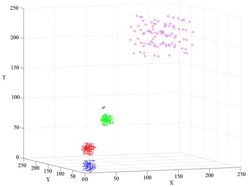
Figure 7. Clustering result of D₁ obtained using STSNN: (a) clustering result with k = 20 and ΔT = 10 and (b) clustering result with k = 20 and ΔT = 20.

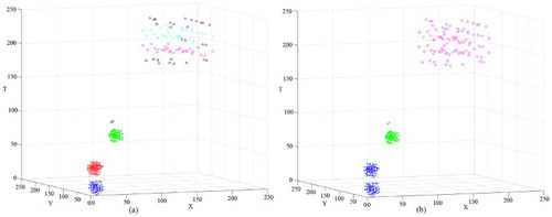
Figure 8. Clustering result of D₁ obtained using ST-DBSCAN: (a) clustering result with Eps = 10 and ΔT = 10 and (b) clustering result with Eps = 20 and ΔT = 20.

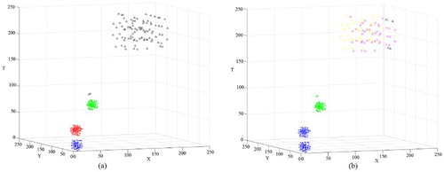
Table 2. Number of clusters of D₁ for different k values.

Values of k	8	10	12	13	14	15	16	17	18	19
Cluster number	16	9	7	7	4	4	4	4	4	4
Values of k	20	…	53	54	…	65	66	67	68	…
Cluster number	4	4	4	3	3	3	2	2	1	…

Table 3. Evaluation results of different clustering algorithms using different indices for D₁.

Index	DBSTC	STSNN		ST-DBSCAN
	Figure 6	Figure 7(a)	Figure 7(b)	Figure 8(a)	Figure 8(b)
CP	11.29	15.17	12.36	5.25	11.50
SP	186.49	161.20	179.56	46.89	177.04
DBI	0.030	0.032	0.053	0.067	0.050

The second data set has three clusters, C₁, C₂ and C₃ (Figure 9). Figure 10 shows two clusters in the temporal domain. To distinguish them, the reachable time windows could both be set to 3. Based on the lifetime of the cluster number (Table 4), k could be set between 15 and 40. The clustering result of DBSTC is shown in Figure 11 for k = 16 and k = 20. For the STSNN algorithm, we also set k = 16 and k = 20, and in both cases, we used ΔT = 3. The two algorithms both correctly distinguished clusters C₁, C₂ and C₃. Compared with DBSTC, STSNN classified more noises into clusters. In addition, STSNN classified the data set into 8 clusters (k = 16) and 11 clusters (k = 20) because of taking isolated noises as core points, whereas DBSTC classified D₂ into 3 clusters when k was appropriate. Thus, the reachable_factor that we proposed can effectively solve the problem of misjudgment of core points that occurred when STSNN was used. As for ST-DBSCAN, it classified D₂ into three clusters when D₂ had clusters with similar dense densities with proper parameters. However, as we can see from Figure 13(a), C₃ is not an ellipsoid of uniform density, the density of out range is less than inside. Thus, ST-DBSCAN did not identified part of points in out range as C₃. In order to classify those points, we need to increase ΔT, which would merge C₂ and C₃ together as shown in Figure 13(b). Table 5 shows the evaluation results of different clustering algorithms using different indices for D₂. The smallest CP, DBI and the largest SP indicate that our algorithm has the best performance.

Figure 9. Original data set D₂ with 2696 points.

Figure 10. The ORTWD of D₂ for ΔT = 3 and MinPts = 20.

Figure 11. Clustering result of D₂ obtained using DBSTC: (a) clustering result for k = 16 and (b) clustering result for k = 20.

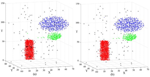
Figure 12. Clustering result of D₂ obtained using STSNN: (a) clustering result for k = 16 and ΔT = 3 and (b) clustering result for k = 20 and ΔT = 3.

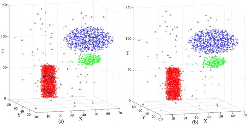
Figure 13. Clustering result of D₂ obtained using ST-DBSCAN: (a) clustering result for Eps = 10 and ΔT = 3.9 and (b) clustering result for Eps = 10 and ΔT = 5.

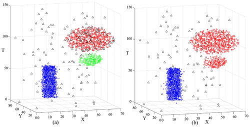
Figure 14. Original data set D₃.

Table 4. Number of clusters of D₂ for different k values.

Values of k	8	10	12	13	14	15	16	17	18	19
Cluster number	129	62	18	8	6	3	3	3	3	3
Values of k	20	21	22	23	24	…	40	…	100	…
Cluster number	3	3	3	3	3	3	3	3	3	…

Table 5. Evaluation results of different clustering algorithms using different indices for D₂.

Index	DBSTC		STSNN		ST-DBSCAN
	Figure 11(a)	Figure 11(b)	Figure 12(a)	Figure 12(b)	Figure 13(a)	Figure 13(b)
CP	5.19	5.13	8.73	12.10	5.98	5.87
SP	35.75	35.79	35.32	31.34	26.22	34.23
DBI	0.014	0.012	0.028	0.020	0.053	0.080

The third data set D₃ contains four clusters with different sizes, shapes and densities (Figure 14). As observed in Figure 15(a), we set the time windows of the 1–2925th points of the ORTWD algorithm’s result to 0.9, the time windows of the 2926–3936th points to 0.5 and the time windows of the 3937–4150th points to 0.5. Based on the lifetime of the cluster number (Table 6), k could be set between 20 and 32. The clustering result of D₃ obtained using DBSTC is shown in Figure 15(b). From the result, it can be seen that DBSTC performed well. Correspondingly, STSNN separated C₄ when ΔT = 1, whereas it merged C₂ and C₃ together when ΔT = 2. ST-DBSCAN had the same problem. The only different is ST-DBSCAN separated C₄ into three clusters and lots of noise points while STSNN separated C₄ into two clusters. Therefore, the performance of DBSTC was not influenced by varied spatiotemporal densities, sizes, shapes and noise of data sets. Table 7 shows the valuation results of different clustering algorithms using different indices for D₃. The smallest DBI and the largest SP indicate the best performance of our algorithm. As for CP, the same situation as for D₁ happens again. The ST-DBSCAN responding Figure 17(a) cannot detect the loosen cluster C₄. It gets the smallest CP because it only has three clusters with a high density. Our algorithm gets the second smallest CP, which indicates good clustering results.

Figure 15. Clustering result of D₃ obtained using DBSTC: (a) the ORTWD of D₃ with ΔT = 4 and MinPts = 50 and (b) clustering result obtained using DBSTC with k = 20.

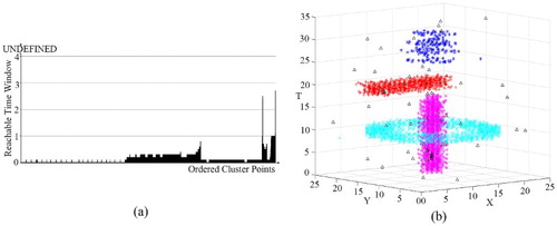
Figure 16. Clustering result of D₃ obtained using STSNN: (a) clustering result with k = 20 and ΔT = 1 and (b) clustering result with k = 20 and ΔT = 2.

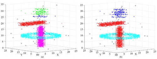
Figure 17. Clustering result of D₃ obtained using ST-DBSCAN: (a) clustering result with Eps = 1 and ΔT = 0.9 and (b) clustering result with Eps = 1 and ΔT = 2.

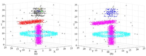
Table 6. Number of clusters in D₃ for different k values.

Values of k	14	15	16	17	18	19	20	21	…	25
Cluster number	21	9	5	7	5	5	4	4	4	5
Values of k	26	…	33	34	…	37	38	39	40	41
Cluster number	4	4	4	5	5	5	4	5	6	6

Table 7. Evaluation results of different clustering algorithms using different indices for D₃.

Index	DBSTC	STSNN		ST-DBSCAN
	Figure 15(b)	Figure 16(a)	Figure 16(b)	Figure 17(a)	Figure 17(b)
CP	2.96	3.11	4.65	2.19	3.46
SP	2.77	2.55	1.90	2.61	1.94
DBI	0.026	0.034	0.101	0.075	0.149

4.2. Real world applications to seismic data sets

Seismicity is a complex dynamic spatiotemporal process with variations in space, time and size over very broad ranges of scales (Zaliapin and Ben-Zion 2013). In this experiment, two seismic data sets were used to test the performance of the DBSTC algorithm for finding clustered earthquakes. Clustered earthquakes are usually perceived as foreshocks (earthquakes that occur before strong ones) or aftershocks (earthquakes that occur after strong ones) of strong earthquakes (Pei et al. 2010), which may help predict strong earthquakes or/and understand their underlying mechanisms (Ripepe, Piccinini, and Chiaraluce 2000).

The study area is around southwestern china (bounds 72–106°E, 20–40°N). This region includes the location of the devastating Wenchuan earthquake (M = 8.2). The data sets were downloaded from the China Earthquake Data Center (http://data.earthquake.cn/data/).

Seismic data set SD₁ has 294 points of earthquakes from 1 May 1975 to 31 May 1976 with magnitudes of greater than 3. The origin data set are shown in Figure 18. Clustering results obtained using DBSTC, STSNN and ST-DBSCAN are shown in Figures 19–21, respectively. Based on the ORTWD (Figure 19(a)), the time windows of the 1–54th points were set to 0.5, the time windows of the 55–138th points were set to 0.4, and the time windows of the 139–294th points were set to 0.3. The DBSTC algorithm detected three clusters, which were labeled as C₁, C₂ and C₃. As shown in Table 8, C₁, C₂ and C₃ represent three clustered strong earthquakes: the Menglian earthquake (which occurred on 12 July 1995 at 21.96°N, 99.16°E, M = 7.3; C₁), the Wuding earthquake (which occurred on 24 October 1995 at 26.02°N, 102.24°E, M = 6.6; C₂) and the Lijiang earthquake (which occurred on 3 February 1996 at 27.34°N, 100.25°E, M = 6.9; C₃). There are 18 points in C₁, and 8 of them were identified as foreshocks of the Menglian earthquake. As for the Wuding earthquake and the Lijiang earthquake, 42 and 85 aftershocks were identified, respectively. This results match well with the seismic records (Chen 2002). As for STSNN, when we chose a smaller ΔT = 0.32, STSNN did identify clusters C₂ and C₃ while failed to detect C₁ which has a loose temporal density. However, while we chose a larger ΔT = 0.64, STSNN detected C₃ while other noise points were identified into clusters and some isolated points were classified as single clusters.ST-DBSCAN could identified three clusters with Eps = 0.2 and ΔT = 1.3, while each cluster is much larger than cluster detected by DBSTC and included some noise points. In order to make each cluster smaller, we decreased ΔT, which did work while C₂ are separated into two clusters.

Figure 18. Seismic data set SD₁: (a) original data set and (b) vertical perspective of the data set.

Figure 19. Clustering result of the seismic data set SD₁ obtained using DBSTC: (a) the ORTWD with ΔT = 1 and MinPts = 20 and (b) clustering result using DBSTC with k = 20.

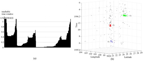
Figure 20. Clustering result of SD₁ obtained using STSNN: (a) clustering result with k = 20 and ΔT = 0.32 and (b) clustering result with k = 20 and ΔT = 0.64.

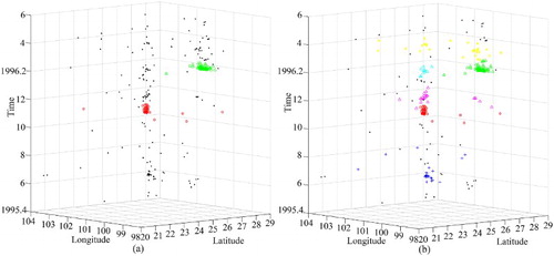
Figure 21. Clustering result of SD₁ obtained using ST-DBSCAN: (a) clustering result with Eps = 0.5 and ΔT = 0.5 and (b) clustering result with Eps = 0.2 and ΔT = 1.3.

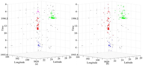
Table 8. Statistical information of the clustering result of the seismic data set SD₁.

Clusters	Number of earthquakes	Names of the strong earthquake	Locations of the strong earthquake	Magnitudes of the strong earthquake
C1	18	Menglian earthquake	21.96°N, 99.16°E	7.3
C2	42	Wuding earthquake	26.02°N, 102.24°E	6.6
C3	85	Lijiang earthquake	27.34°N, 100.25°E	6.9

Seismic data set SD₂ has 1131 points of earthquakes from 21 January 2008 to 23 February 2010 with magnitudes greater than 4 in an area located between 72° and 106°E and 30° and 40°N. Figure 22 shows the original data set, and Figures 23–25 show the clustered results obtained using DBSTC, STSNN and ST-DBSCAN, respectively. The time windows of the 1–1016th points were set to 1, the time windows of the 1017–1054th points were set to 2, and the time windows of the 1054–1131th points were set to 1.5 based on the ORTWD (Figure 18(a)). The proposed DBSTC algorithm detected seven clusters, labeled as C₁–C₇. Cluster C₂ occurred after the Wenchuan earthquake (on 12 May 2008 at 31.01°N, 103.42°E, M = 8.2), and 734 earthquakes were identified as aftershocks of the Wenchuan earthquake. The 56 earthquakes identified as C₃ contain 3 foreshocks and 53 aftershocks of the Wuqia earthquake (which occurred on 5 October 2008). One earthquake of C₄ was identified as a foreshock of the Zhongba earthquake (which occurred on 24 October 1995 at 30.92°N, 80.57°E, M = 6.9), and the rest were identified as aftershocks. There are 38 earthquakes in C₅, and 4 of them were identified as foreshocks of the Tanggula earthquake (which occurred on 10 June 2008 at 33.10°N, 92.07°E, M = 5.5). C₆ was identified as aftershocks of the Yutian earthquake (which occurred on 20 March 2008). Two strong earthquakes in Dachaidan on 10 November 2008 and 28 August 2009 were identified as Dachaidan^a and Dachaidan^b, respectively. C₁ and C₇ were used to identify the aftershocks of these two strong earthquakes. Statistical information of the clustered earthquakes is listed in Table 9. According to the seismic records (Li, Liu, and Yu 2009; Li et al. 2010; Ji et al. 2011), there are seven strong earth quakes occurred during this period thus our clustering results are reasonable. As for STSNN, there are 17 clustered earthquakes with ΔT = 1.7 and 14 clustered earthquakes with ΔT = 2.56. STSNN makes a lot of isolated point into core point and identified some small clusters no matter which ΔT we choose. When we chose a smaller ΔT, STSNN identified more noise points as clusters and cut the clustered earthquakes of Wenchuan into three clusters. If we chose a larger ΔT, STSNN made each cluster much more larger than DBSTC while it still classified clustered earthquakes of Wenchuan into two parts. This is caused by fixed time windows in varied temporal densities while our algorithm can solve it. ST-DBSCAN does not have the isolated core point problem compared with STSNN. When Eps = 5 and ΔT = 2, ST-DBSCAN identified seven clusters. Several clusters are bit larger than the result of DBSTC and included some noise points such as C₂, C₆ and C₇. In order to decrease the number of points in clusters, we decreased ΔT = 2, which excluded some noise points while C₂ were separated into two clusters.

Figure 22. Seismic data set SD₂: (a) original data set and (b) vertical perspective of data set.

Figure 23. Clustering result of the seismic data set SD₂ obtained using DBSTC: (a) ORTWD with ΔT = 3 and MinPts = 30 and (b) clustering result obtained using DBSTC with k = 20.

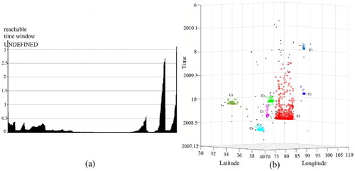
Figure 24. Clustering result of SD₂ obtained using STSNN: (a) clustering result with k = 20 and ΔT = 1.7 and (b) clustering result with k = 20 and ΔT = 2.56.

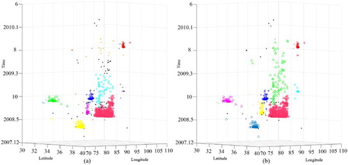
Figure 25. Clustering result of SD₂ obtained using ST-DBSCAN: (a) clustering result with Eps = 5 and ΔT = 1 and (b) clustering result with Eps = 5 and ΔT = 2.

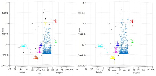
Table 9. Summary of clustering results with seismic data set SD₂.

Clusters	Number of earthquakes	Names of the strong earthquake	Locations of the strong earthquake	Magnitude of the strong earthquake
C1	15	Dachaidan^a earthquake	37.66°N, 95.91°E	6.6
C2	735	Wenchuan earthquake	31.01°N, 103.42°E	8.2
C3	57	Wuqia earthquake	39.58°N, 73.67°E	7.0
C4	47	Zhongba earthquake	30.92°N, 83.57°E	6.9
C5	39	Tanggula earthquake	33.10°N, 92.07°E	5.5
C6	93	Yutian earthquake	35.64°N, 81.54°E	7.5
C7	50	Dachaidan^b earthquake	37.60°N, 95.90°E	6.6

5. Conclusions and future works

Most density-based clustering methods cannot be applied to data sets that contain clusters with different densities in both the spatial and temporal domains. In this article, we proposed the DBSTC algorithm to solve the clustering problem for such data sets. We proposed the notion of reachable_factor to solve the clustering problem for data sets with different spatial densities and the ORTWD algorithm to solve the clustering problem for data sets with varied densities in the temporal domain. To demonstrate the efficiency of our algorithm, several simulated data sets were used to compare our algorithm with STSNN and ST-DBSCAN. The comparison results show that the DBSTC algorithm was able to discover spatiotemporal clusters with different densities, whereas STSNN and ST-DBSCAN failed. In addition, our algorithm was also effectively applied to classify data sets containing clusters with different sizes and shapes in the presence of noises. Finally, the DBSTC algorithm was successfully applied to identify foreshocks and aftershocks in southwestern China using the real world seismic data sets. Such real world applications may help researchers understand the mechanisms underlying the earthquakes.

This algorithm may encounter computation bottlenecks with tremendous data sets by using use k-NN search, which requires high computational efforts. Future work will focus on further testing the performance of this algorithm. With increase of the amount of available spatiotemporal data, an indexed mechanism or a paralleled method may be needed to improve the efficiency of DBSTC. In addition, the DBSTC algorithm may be applied to some geographic information data sets, such as criminal data sets and disease data sets (Musenge et al. 2013) to help understand the spatiotemporal mechanisms underlying these phenomena.

Acknowledgements

We thank the CyberGIS Center in University of Illinois at Urbana-Champaign for great help and the great suggestions of the reviewers.

Disclosure statement

No potential conflict of interest was reported by the authors.

ORCID

Zhenhong Du http://orcid.org/0000-0001-9449-0415

Yuhua Gu http://orcid.org/0000-0002-8707-8200

Feng Zhang http://orcid.org/0000-0003-1475-8480

Renyi Liu http://orcid.org/0000-0003-4001-4266

Additional information

Funding

This work was supported by the National Natural Science Foundation of China [grant numbers 41671391, 41471313]; the Science and Technology Project of Zhejiang Province [grant numbers 2014C33G20, 2013C33051]; and Major Program of China High Resolution Earth Observation System [grant number 07-Y30B10-9001].

References

- Ana, L. N. F., and Anil K Jain. 2003. “Robust Data Clustering.” Paper presented at the Proceedings of the IEEE Computer Society Conference on Computer Vision and Pattern Recognition, 2003.
- Ankerst, Mihael, Markus M. Breunig, Hans-Peter Kriegel, and Jörg Sander. 1999. “OPTICS: Ordering Points to Identify the Clustering Structure.” Paper presented at the ACM Sigmod Record.
- Biçici, Ergun, and Deniz Yuret. 2007. “Locally Scaled Density Based Clustering.” Paper presented at the International Conference on Adaptive and Natural Computing Algorithms.
- Birant, Derya, and Alp Kut. 2007. “ST-DBSCAN: An Algorithm for Clustering Spatial-Temporal Data.” Data & Knowledge Engineering 60 (1): 208–221. doi: 10.1016/j.datak.2006.01.013
- Byers, Simon, and Adrian E. Raftery. 1998. “Nearest-Neighbor Clutter Removal for Estimating Features in Spatial Point Processes.” Journal of the American Statistical Association 93 (442): 577–584. doi: 10.1080/01621459.1998.10473711
- Campello, Ricardo J. G. B., Davoud Moulavi, and Jörg Sander. 2013. “Density-Based Clustering Based on Hierarchical Density Estimates.” Paper presented at the Pacific-Asia Conference on Knowledge Discovery and Data Mining.
- Chen, Qifu. 2002. Earthquake Cases in China (1995–1996). Beijing: Seismological Press (in Chinese).
- Craglia, Max, Kees de Bie, Davina Jackson, Martino Pesaresi, Gábor Remetey-Fülöpp, Changlin Wang, Alessandro Annoni, et al. 2012. “Digital Earth 2020: Towards the Vision for the Next Decade.” International Journal of Digital Earth 5 (1): 4–21. doi: 10.1080/17538947.2011.638500
- Du, Zhenhong, Yuhua Gu, Chuanrong Zhang, Feng Zhang, Renyi Liu, Jean Sequeira, and Weidong Li. 2017. “ParSymG: A Parallel Clustering Approach for Unsupervised Classification of Remotely Sensed Imagery.” International Journal of Digital Earth 10: 471–489. doi: 10.1080/17538947.2016.1229818
- Elnekave, Sigal, Mark Last, and Oded Maimon. 2007. “Incremental Clustering of Mobile Objects.” Paper presented at the IEEE 23rd International Conference on Data Engineering Workshop, Istanbul, Turkey, April 15, 16, 20.
- Ertoz, Levent, Michael Steinbach, and Vipin Kumar. 2002. “A New Shared Nearest Neighbor Clustering Algorithm and Its Applications.” Paper presented at the Workshop on Clustering High Dimensional Data and its Applications at 2nd SIAM International Conference on Data Mining, Arlington, VA, April 13.
- Ester, Martin, Hans-Peter Kriegel, Jörg Sander, and Xiaowei Xu. 1996. “A Density-Based Algorithm for Discovering Clusters in Large Spatial Databases with Noise.” Paper presented at the KDD.
- Fan, Yida, Qi Wen, and Shirong Chen. 2012. “Engineering Survey of the Environment and Disaster Monitoring and Forecasting Small Satellite Constellation.” International Journal of Digital Earth 5 (3): 217–227. doi: 10.1080/17538947.2011.648540
- Goodchild, Michael F. 2007. “Citizens as Sensors: The World of Volunteered Geography.” GeoJournal 69 (4): 211–221. doi: 10.1007/s10708-007-9111-y
- Goodchild, Michael F., Huadong Guo, Alessandro Annoni, Ling Bian, Kees de Bie, Frederick Campbell, Max Craglia, et al. 2012. “Next-generation Digital Earth.” Proceedings of the National Academy of Sciences USA 109 (28): 11088–11094. doi: 10.1073/pnas.1202383109
- Guo, Huadong. 2012. “Digital Earth: A New Challenge and New Vision.” International Journal of Digital Earth 5 (5): 1–3. doi: 10.1080/17538947.2012.646005
- Ji, Ping, Gang Li, Jie Liu, and Sidao Ni. 2011. “A Review of Seismicity in 2010.” Earthquake Research in China. 25 (1): 111–119.
- Karami, Amin, and Ronnie Johansson. 2014. “Choosing DBSCAN Parameters Automatically Using Differential Evolution.” International Journal of Computer Applications 91 (7). doi: 10.5120/15890-5059
- Kriegel, Hans-Peter, Peer Kröger, Jörg Sander, and Arthur Zimek. 2011. “Density-based Clustering.” Wiley Interdisciplinary Reviews: Data Mining and Knowledge Discovery 1 (3): 231–240.
- Li, Gang, Jie Liu, Ping Ji, and Tieshuan Guo. 2010. “A Review of Seismicity in 2009.” Earthquake Research in China 24 (1): 137–146.
- Li Gang, Jie Liu, and Surong Yu. 2009. “A Review of Seismicity in 2008.” Earthquake Research in China 23 (1): 105–118.
- Liu, Qiliang, Min Deng, Jiantao Bi, and Wentao Yang. 2014. “A Novel Method for Discovering Spatio-temporal Clusters of Different Sizes, Shapes, and Densities in the Presence of Noise.” International Journal of Digital Earth 7 (2): 138–157. doi: 10.1080/17538947.2012.655256
- Liu, Shuo, Xiangtao Fan, Qingke Wen, Wei Liang, and Yuanfeng Wu. 2014. “Simulated Impacts of 3D Urban Morphology on Urban Transportation in Megacities: Case Study in Beijing.” International Journal of Digital Earth 7 (6): 470–491. doi: 10.1080/17538947.2012.740079
- Matsuda, Yoshitatsu, Kazunori Yamaguchi, and Ken-Ichiro Nishioka. 2015. “Discovery of Regular and Irregular Spatio-temporal Patterns from Location-Based SNS by Diffusion-type Estimation.” IEICE TRANSACTIONS on Information and Systems E98.D (9): 1675–1682. doi: 10.1587/transinf.2015EDP7095
- McArdle, Gavin, Ali Tahir, and Michela Bertolotto. 2015. “Interpreting Map Usage Patterns Using Geovisual Analytics and Spatio-temporal Clustering.” International Journal of Digital Earth 8 (8): 599–622. doi: 10.1080/17538947.2014.898704
- Miller, Harvey J., and Jiawei Han. 2009. Geographic Data Mining and Knowledge Discovery. Boca Raton: CRC Press.
- Musenge, Eustasius, Tobias Freeman Chirwa, Kathleen Kahn, and Penelope Vounatsou. 2013. “Bayesian Analysis of Zero Inflated Spatiotemporal HIV/TB Child Mortality Data Through the INLA and SPDE Approaches: Applied to Data Observed Between 1992 and 2010 in Rural North East South Africa.” International Journal of Applied Earth Observation and Geoinformation 22: 86–98. doi: 10.1016/j.jag.2012.04.001
- Northrop, Paul. 1998. “A Clustered Spatial-Temporal Model of Rainfall.” Proceedings of the Royal Society A: Mathematical, Physical and Engineering Sciences 454 (1975): 1875–1888. doi: 10.1098/rspa.1998.0238
- Pei, Tao, Chenghu Zhou, A-Xing Zhu, Baolin Li, and Chengzhi Qin. 2010. “Windowed Nearest Neighbour Method for Mining Spatio-temporal Clusters in the Presence of Noise.” International Journal of Geographical Information Science 24 (6): 925–948. doi: 10.1080/13658810903246155
- Pei, Tao, A-Xing Zhu, Chenghu Zhou, Baolin Li, and Chengzhi Qin. 2006. “A New Approach to the Nearest-Neighbour Method to Discover Cluster Features in Overlaid Spatial Point Processes.” International Journal of Geographical Information Science 20 (2): 153–168. doi: 10.1080/13658810500399654
- Ripepe, M., D. Piccinini, and L. Chiaraluce. 2000. “Foreshock Sequence of September 26th, 1997 Umbria-Marche Earthquakes.” Journal of Seismology 4 (4): 387–399. doi: 10.1023/A:1026508425230
- Vahidnia, Mohammad H., Ali A. Alesheikh, Saeed Behzadi, and Sara Salehi. 2013. “Modeling the Spread of Spatio-temporal Phenomena Through the Incorporation of ANFIS and Genetically Controlled Cellular Automata: A Case Study on Forest Fire.” International Journal of Digital Earth 6 (1): 51–75. doi: 10.1080/17538947.2011.603366
- Wang, Qinjun, Huadong Guo, Yu Chen, Qizhong Lin, and Hui Li. 2011. “Application of Remote Sensing for Investigating Mining Geological Hazards.” International Journal of Digital Earth 6 (5): 1–20.
- Wang, Min, Aiping Wang, and Anbo Li. 2006. “Mining Spatial-Temporal Clusters from Geo-databases.” In Advanced Data Mining and Applications, Xi’an, China, August 14–16, 2006, edited by Xue Li, Osmar R. Zaiane, and Zhanhuai Li, 263–270. Berlin: Springer Berlin Heidelberg.
- Woudsma, Clarence, John F. Jensen, Pavlos Kanaroglou, and Hanna Maoh. 2008. “Logistics Land Use and the City: A Spatial-temporal Modeling Approach.” Transportation Research Part E: Logistics and Transportation Review 44 (2): 277–297. doi: 10.1016/j.tre.2007.07.006
- Xue, Cunjin, Wanjiao Song, Lijuan Qin, Qing Dong, and Xiaoyang Wen. 2015. “A Spatiotemporal Mining Framework for Abnormal Association Patterns in Marine Environments with a Time Series of Remote Sensing Images.” International Journal of Applied Earth Observation and Geoinformation 38: 105–114. doi: 10.1016/j.jag.2014.12.009
- Yusof, Norhakim, and Raul Zuritamilla. 2017. “Mapping Frequent Spatio-temporal Wind Profile Patterns Using Multi-Dimensional Sequential Pattern Mining.” International Journal of Digital Earth 10: 238–256. doi: 10.1080/17538947.2016.1217943
- Zaliapin, I., and Y. Ben-Zion. 2013. “Earthquake Clusters in Southern California II: Classification and Relation to Physical Properties of the Crust.” Journal of Geophysical Research: Solid Earth 118 (6): 2865–2877. doi:10.1002/jgrb.50178.
- Zaliapin, Ilya, Andrei Gabrielov, Vladimir Keilis-Borok, and Henry Wong. 2008. “Clustering Analysis of Seismicity and Aftershock Identification.” Physical Review Letters 101 (1): 018501. doi: 10.1103/PhysRevLett.101.018501