A disaggregation approach for estimating high spatial resolution broadband emissivity for bare soils from Landsat surface reflectance

ABSTRACT

High spatial resolution land surface broadband emissivity (BBE) is not only useful for surface energy balance studies at local scales, but also can bridge the gap between existing coarser resolution BBE products and point-based field measurements. This study proposes a disaggregation approach that utilizes the established BBE–reflectance relationship for estimating high spatial resolution BBE for bare soils from Landsat surface reflectance data. The disaggregated BBE is compared to the BBE calculated from spatial–temporal matched Advanced Spaceborne Thermal Emission and Reflectance Radiometer emissivity product. Comparison results show that better agreement is achieved over relative homogeneous areas, but deteriorated over heterogeneous and cloud-contaminated areas. In addition, field-measured emissivity data over large homogeneous desert were also used to validate the disaggregated BBE, and the bias is 0.005. The comparison and validation results indicated that the disaggregation approach can obtain high spatial resolution BBE with better accuracy for homogeneous area.

KEYWORDS:

• Broadband emissivity
• ASTER
• TM
• bare soil
• disaggregation

1. Introduction

Land surface broadband emissivity (BBE) is a key parameter for estimating land surface radiation budget (SRB), which is the driving force of many land surface processes (e.g. ecological, hydrological, biogeochemical) (Liang et al. 2010; Dickinson 1995; Xue et al. 1998). Due to limited observations, BBE has been crudely treated in the land surface models or the land surface schemes in the global circulation models (Bonan et al. 2002; Dai et al. 2003), which has hindered the further improvement of simulation accuracy of these models (Zhou, Dickinson, Tian, et al. 2003). A study of the sensitivity of simulated energy balance to changes in BBE over North Africa and the Arabian Peninsula showed that a decrease of 0.1 in the soil BBE increased the ground and air temperatures by an average of approximately 1.1°C and 0.8°C, respectively, while decreases in the net and upward longwave radiation were about 6.6 and 8.1 W/m², respectively (Zhou, Dickinson, Tian, et al. 2003). Fortunately, a more realistic satellite-derived BBE can improve the simulation results of climate models (Jin and Liang 2006).

There are three types of methods that can be used to produce BBE from satellite data. The first is classification-based method. Wilber, Kratz, and Gupta (1999) generated a global BBE (5–100 μm) map with a 10 min spatial resolution for satellite retrievals of longwave radiation by assigning constant emissivity values to International Geosphere–Biosphere Program land cover types. The second is named as spectral conversion, i.e. converting narrowband emissivities (NBEs) to BBE using a linear function. For example, Ogawa et al. (2008) mapped the global monthly BBE (8–13.5 μm) by converting the Moderate-resolution Imaging Spectroradiometer (MODIS) NBEs (approximately 5 km), and a North African BBE (8–13.5 μm) using the Advanced Spaceborne Thermal Emission and Reflectance Radiometer (ASTER) NBEs (90 m). The third approach uses optical (from visible to shortwave infrared, VIS-SWIR) reflectance data to estimate BBE. For example, Cheng and Liang link ASTER BBE (8–13.5 μm) and seven MODIS spectral albedos for non-vegetated surfaces at 1 km spatial resolution, and use this linkage to derive the BBE from MODIS spectral albedos (Cheng and Liang 2014). With the aforementioned methods, we can obtain BBE with spatial resolution ranging from 90 m to 10 min. Methods of the third category mentioned above have been adopted to produce operational global BBE product with spatial–temporal resolutions of eight-day, 1 km and 0.05° from MODIS and Advanced Very High Resolution Radiometer (AVHRR) optical data from 1981 to 2015 (Liang et al. 2013), which is freely available to public (ftp://ftp.glcf.umd.edu/glcf/GLASS/EMT/).

A large number of studies have been conducted to retrieve the key variables or components of SRB from Landsat data, for example, albedo (Shuai et al. 2011), shortwave net radiation (Wang, Liang, and He 2014) and land surface temperature (Sobrino, Jimenez-Munoz, and Paolini 2004). To our knowledge, no studies are conducted to estimate BBE from Landsat data. Landsat Thematic Mapper (TM)/ETM⁺ only has one channel in thermal infrared (TIR); it is impossible to derive the BBE accurately, especially for bare soil whose BBE varies with surface conditions. However, such data are indispensable for surface energy balance studies at local scales thereby improving our understanding of land–atmosphere interactions (Ogawa and Schmugge 2004; French et al. 2005; Liang et al. 2010; Anderson et al. 2011). Moreover, the derived finer resolution BBE can bridge the gap between existing coarser resolution BBE products and point-based field measurements and be used for validating coarse-resolution data.

Disaggregation is a powerful method for improving the spatial resolution of high-level remote sensing product, which has been widely used in improving the spatial resolution of essential land surface variables, such as land surface temperature (Agam et al. 2007; Kustas et al. 2003), soil moisture (Choi and Hur 2012), evapotranspiration (Anderson et al. 2011), and leaf area index (Wu, Tang, and Li 2013). The key point of these disaggregation approaches is to establish a unique relationship between the target variable and predictor variable at coarse scale that could be applied to imagery at the finer pixel resolution (Wu and Li 2009; Zhan et al. 2013). The purpose of this study is to design a disaggregation approach for estimating the 30 m BBE from Landsat surface reflectance.

2. Data and method

2.1. Satellite data

A area of 520 × 1400 km² in North Africa that covers Algeria, Libya and Tunisia was selected as the study area in this study (Zhou, Dickinson, Ogawa, et al. 2003). Landsat 5 TM data from 2001 to 2002 were downloaded from United States Geological Survey Earth Resource Observation and Science Center (http://glovis.usgs.gov/). The downloaded TM data have been processed by the Landsat Ecosystem Disturbance Adaptive Processing System (Masek et al. 2006) released by National Aeronautics and Space Administration Goddard Space Flight Center to obtain the cloud mask and surface reflectance. The TM data with less than 50% cloud cover were considered. The revisit period of TM is 16 days, and the spatial resolution of TM reflective bands is 30 m. The spectral characteristics of TM are shown in Table 1.

Table 1. The spectral characteristic of TM reflective bands and ASTER TIR bands.

TM		ASTER
Channels	Spectral coverage (μm)	Channels	Spectral coverage (μm)
1	0.45–0.53	10	8.13–8.48
2	0.52–0.60	11	8.48–8.33
3	0.63–0.69	12	8.93–9.28
4	0.76–0.90	13	10.25–10.95
5	1.55–1.75	14	10.95–11.65
7	2.08–2.35	–	–

ASTER obtains high-resolution (15–90 m² per pixel) images of the earth in 14 different wavelengths of the electromagnetic spectrum, ranging from visible to TIR light (Abrams 2000). ASTER has five channels in the TIR region (Table 1). The ASTER surface emissivity products (AST_05) provide five NBEs in the spectral domain of 8–12 µm with a spatial resolution of 90 m. AST_05 was derived from the temperature/emissivity separation (TES) algorithm (Gillespie et al. 1998). The TES algorithm combines the advantages of the normalized emissivity method, the spectral ratio method, and the minimum–maximum difference method and adds certain external constraints. Through optimization, an effect of stepwise refinement is achieved. The ASTER TES algorithm-based temperature retrieval has an error of approximately ±1.5 K; the error for the NBEs is approximately ±0.015. ASTER emissivity datasets are proven to be relatively accurate and have little seasonal variation in arid areas (Hulley and Hook 2009; Sabol et al. 2009; Gillespie et al. 2011; Kato, Matsunaga, and Tonooka 2014). AST_05 from 2001 to 2002 was downloaded from https://search.earthdata.nasa.gov/.

2.2. In situ measurements

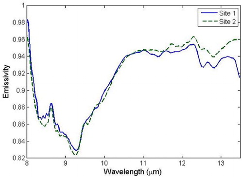
We did not acquire the synchronized in situ measurements from the study area. The field-measured emissivity spectra derived from a field experiment conducted on 6 June 2011 in the Taklimakan Desert (Cheng et al. 2014) were used to test the performance of the disaggregated BBE over homogeneous area. The Taklimakan Desert is the largest active desert in China and the second largest in the world. It lies in a depression between two high, rugged mountain ranges. Two flat and homogeneous sand sites in the central area of the Taklimakan Desert were selected. The Model 102 Portable FT-IR Spectrometer and a Labsphere gold plate were used to measure spectral radiance emitted by the target and by the environment under a clear sky, from which the emissivity spectra of the site were derived by the iterative spectrally smooth temperature and emissivity separation algorithm (Borel 2008). Figure 1 shows the derived emissivity spectra. For the detailed information of the field measurements, please refer to Cheng et al. (2014).

Figure 1. Field-measured emissivity spectra of sites 1 and 2 at the central part of the Taklimakan Desert.

2.3. Exploring the linkage between BBE and reflectance

The linkages between TIR parameter and optical parameter have been discovered long before. Menenti et al. (1989) reported a linear relationship between field-measured surface temperature and reflectance over non-homogeneous surface types (western desert of Egypt). Van De Griend and Owe (1993) found that emissivity has a good logarithmic relationship with the normalized difference vegetation index (NDVI). Olioso (1995) noted that this relationship is closely related to soil emissivity, the component effective emissivity of leaves, canopy structure, the optical features of leaves, solar position and the proportion of soil penetrated by sunlight but is insensitive to observational geometric conditions. Recently, Cheng and Liang established a linear relationship between BBE and seven MODIS spectral albedos (Cheng and Liang 2014), and a nonlinear relationship between BBE and AVHRR visible and near-infrared reflectance (Cheng and Liang 2013).

Those studies indicated that the empirical relationships between emissive and optical variables existed. Thus, we first established the empirical relationship between BBE derived from ASTER emissivity product and Landsat TM5 VIS-SWIR reflectance at 1 km scale, and then calculated the BBE at scale of Landsat reflectance product, assuming that the empirical relationship at 1 km can be applied to the fine scale of Landsat TM5.

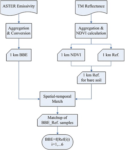
Figure 2 shows the flowchart of exploring the linkage between ASTER BBE and TM surface reflectance at 1 km resolution. Firstly, ASTER data were rotated back to the original angle and projected to the UTM projection. Then ASTER emissivity was converted to BBE at 8–13.5 μm using the formula (Cheng et al. 2013):(1) where is the BBE, are the five ASTER NBEs. Then the BBE was aggregated to 1 km spatial resolution using area weighting method (Liu, Hiyama, and Yamaguchi 2006). Secondly, the TM surface reflectance was also aggregated to 1 km spatial resolution and the NDVI was calculated using TM channels 3 and 4. An NDVI threshold of 0.2 was used to identify the bare soil pixels (Sobrino et al. 2008). Thirdly, the matchup of BBE–reflectance were extracted from the spatial–temporal matched the ASTER BBE and TM surface reflectance. In the spatial–temporal match, the overpass time of the ASTER data was assigned as a reference, and the TM data were selected as temporal matched if the difference of the overpass time of the TM and the ASTER was less than eight days. The spatial math was completed based on the Euclidean distance between pixels. Finally, the linear relationship between BBE and reflectance at 1 km spatial resolution was established by linear regression using the extracted BBE–reflectance pairs. Then the established relationship was applied to TM surface reflectance to estimate 30 m BBE.

Figure 2. The flowchart for establishing the relationship between BBE and reflectances at 1 km spatial resolution.

3. Results

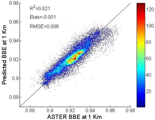
Totally, 26,812 samples were extracted from spatial–temporal matched relative homogeneous ASTER and TM image pairs in 2002 over the study area. These samples were used to establish the linear relationship between BBE and surface reflectance by linear regression. The fitted formula was presented as follows:(2) where is the BBE and is the surface reflectance of Landsat TM5 for channel . The determination coefficient was 0.821. The bias and root mean square error (RMSE) were –0.001 and 0.006, respectively. The fitting result is shown in Figure 3.

Figure 3. Comparison of ASTER BBE and that predicted by Equation (2) from TM surface reflectance.

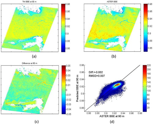
We obtained two pairs of matched ASTER and TM images in 2001 over the study area and used to test the developed disaggregation approach. The images of the first pair are shown in Figure 4. The imagery is clearly non-vegetated. Only scatter clouds are distributed at the upper-left and down-right corner. The black color in the middle may be the bare soil, whereas the white and yellow colors in the top and bottom of the image are likely to be sands. The retrieved BBE is shown in Figure 5. Soil BBEs are around 0.93 and sand BBEs are approximately 0.90. The retrieved 30 m BBE was aggregated to 90 m and compared to the BBE calculated from the ASTER emissivity product (AST05). Figure 6 shows the comparison results. They agree well with each other in spatial pattern and the difference is quite small. The average difference was –0.002 and the root mean error of difference (RMSD) was 0.007.

Figure 4. The first pair of spatial–temporal matched TM and ASTER images. (a) The true color composition of TM data using bands 3, 2 and 1 (color version of the figure is available online). (b) Gray map of ASTER band 12.

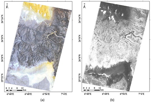
Figure 5. The 30 BBE retrieved from TM surface reflectance.

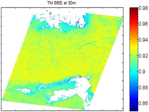
Figure 6. Comparison between retrieved TM BBE and ASTER BBE. (a) TM 90 m BBE aggregated from the retrieved 30 m BBE; (b) ASTER BBE; (c) the difference map of TM and ASTER 90 m BBE and (d) scatter plot of the difference.

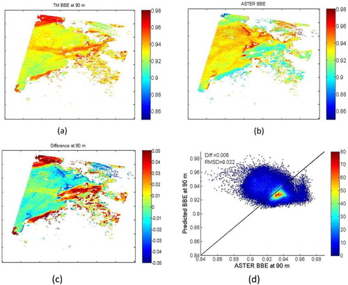
Another pair of ASTER and TM images is shown in Figure 7. This pair of image seems more heterogeneous than the first pair. Besides, there are many missing values in both images resulting from the cloud contamination. The black color in the TM images may be the mixture of soil and sand, and less contaminated by cloud. The retrieved BBE is shown in Figure 8. The number of the effective BBEs accounts for less than 50% of the whole data. Larger difference is present in the comparison results (Figure 9), especially at the border and cloud-contaminated area. Except for these areas, the consistency between the retrieved BBE and ASTER BBE is not bad. The average difference was 0.006 and the RMSD was 0.022.

Figure 7. Another pair of spatial–temporal matched TM and ASTER images. (a) The true color composition of TM data using bands 3, 2 and 1 (color version of the figure is available online). (b) Gray map of ASTER band 12.

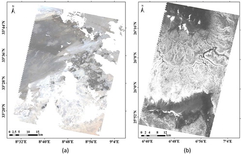
Figure 8. The 30 m BBE retrieved from TM surface reflectance.

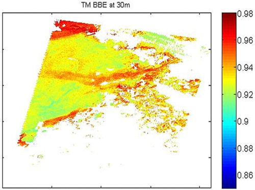
Figure 9. Comparison between retrieved TM BBE and ASTER BBE. (a) TM 90 m BBE aggregate from the retrieved 30 m BBE; (b) ASTER BBE; (c) the difference map of TM and ASTER 90 m BBE and (d) scatter plot of the difference.

The disaggregation approach was also validated with the field-measured emissivity spectra in Section 2.3. The measured emissivity spectra were converted to BBE and the corresponding values are 0.924 and 0.922. The matched TM data were used to calculate the BBE with Equation (2), and the values of 0.930 and 0.926 were obtained. The bias is 0.005. The test and validation results are consistent, i.e. the disaggregation approach can obtain high spatial resolution BBE with better accuracy for homogeneous area. Note that differences (residuals) between original BBE (1 km) and the disaggregated BBEs (30 m) aggregated to the original spatial resolution always exist because the fitted relationship is imperfect and the surface reflectance cannot provide all the information required to reconstruct BBE at finer spatial resolutions. The residues are redistributed over the disaggregated variables to enforce energy conservation in previous studies (Gao, Kustas, and Anderson 2012). Although the residual redistribution may improve the disaggregated results, it yields no new information about the sub-pixel variation which comes from the established relationship. Thus, the above comparison and validation results come from the disaggregated results without redistributing the residues.

4. Discussion

Previous studies have demonstrated that there is an empirical relationship between BBE and surface VIS-SWIR reflectance. However, whether there is a physical linkage remains unclear. Taking the method of Cheng et al. (2013), we generated the Mie parameters (single-scattering albedo and the asymmetry factor) for single mineral particle in the spectral range of 0.44–13.5 μm by virtue of the Mie code (Mie 1908) using the optical constants of 42 mineral samples collected from the Jean-St. Petersburg database of optical constants (http://www.astro.spbu.ru/JPDOC/f-dbase.html). Then, surface emissivity and reflectance spectra of minerals were simulated using the radiative transfer model of Hapke (1993), from which the BBE and Landsat TM5 VIS-SWIR reflectance were calculated. Assuming that the particles emit and scatter isotropically, the expressions of Hapke reflective and emissive model are given as follows:(3) (4) where and are hemisphere-directional reflectance and directional emissivity; and are viewing zenith angle; and are the particle single-scattering albedo.

A significant multiple linear relationship between BBE and Landsat TM5 VIS-SWIR reflectance was derived, with determination coefficient, bias and RMSE of 0.811, 0.001 and 0.006, respectively. Since minerals are one of primary components of bare soils and rocks, we believe that there is a physical basis between BBE and VIS-SWIR reflectance to some extent.

Since BBE has a close relationship with VIS-SWIR reflectance over bare soils, it is intuitive to make use of such relationship to derive high-resolution BBE using ASTER data. We think this proposal deserves to try but not the scope of this study. It is absolutely essential to derive high-resolution BBE from Landsat data. The reasons are as follows: (1) the Landsat satellites provide the longest temporal record (over 40 years) of land surface observations (Wulder et al. 2016) and Landsat-8 is continuing this legacy, whereas ASTER has approximately 16 years’ data. (2) The Landsat surface reflectance datasets are consistent over the Landsat sensor series (Roy et al. 2015; Claverie et al. 2015). The developed method can be easily extended to other sensors, like ETM⁺. (3) The Landsat archive has been opened at no cost to the scientific community since 2009 (Woodcock et al. 2008). We are trying the study of disaggregating ASTER BBE. Even we can obtain 30 m BBE from ASTER data; we are left with no alternative regarding the 30 m BBE before the year 2000.

5. Conclusion

This study proposes a disaggregation approach for estimating high spatial resolution BBE from Landsat reflective bands for bare soil. First, the linkage between BBE and surface reflectance was established at 1 km using spatial–temporal matched ASTER emissivity and Landsat TM5 surface reflectance products over the North Africa. The established relationship is significant under the level of 0.05. The determination coefficient was 0.821; the bias and RMSE were 0.001 and 0.006, respectively. Then this approach was tested by comparing the retrieved BBE with the BBE calculated from the ASTER emissivity product. Over the relative homogeneous image, better results were achieved with average difference of –0.002 and RMSD of 0.007, respectively. Regarding the heterogeneous and cloud-contaminated image, the results deteriorated, with average difference of 0.006 and RMSD of 0.022, respectively. Finally, two field-measured emissivity spectra over large homogeneous sand of the Desert were used to validate the retrieved BBE. They agree well with each other and the bias is 0.005. The test and validation results indicated that the disaggregation approach can obtain high spatial resolution BBE with better accuracy for homogeneous area.

We are elaborating the approach for estimating 30 m BBE from Landsat TM5 data over vegetated surfaces. Along with the study in this paper, we are able to provide 30 m BBE data, and contribute to the studies of surface energy balance at the local scale.

Acknowledgements

The Landsat data were downloaded from http://glovis.usgs.gov/ and ASTER data were obtained from https://wist.echo.nasa.gov/api/.

Disclosure statement

No potential conflict of interest was reported by the authors.

Additional information

Funding

This work was supported by the National Natural Science Foundation of China [grant number 41371323] and the National Key Research and Development Program of China [grant number 2016YFA0600101].

References

- Abrams, M. 2000. “The Advanced Spaceborne Thermal Emission and Reflection Radiometer (ASTER): Data Products for the High Spatial Resolution Imager on NASA’s Terra Platform.” International Journal of Remote Sensing 21 (5): 847–859. doi: 10.1080/014311600210326
- Agam, N., W. P. Kustas, M. C. Anderson, F. Li, and C. M. U. Neale. 2007. “A Vegetation Index Based Technique for Spatial Sharpening of Thermal Imagery.” Remote Sensing of Environment 107: 545–558. doi: 10.1016/j.rse.2006.10.006
- Anderson, M. C., W. P. Kustas, J. M. Norman, C. R. Hain, J. R. Mecikalski, L. Schultz, M. P. Gonzalez-Dugo, et al. 2011. “Mapping Daily Evapotranspiration at Field to Continental Scales Using Geostationary and Polar Orbiting Satellite Imagery.” Hydrology and Earth System Sciences 15: 223–239. doi: 10.5194/hess-15-223-2011
- Bonan, Gordon B., Keith W. Oleson, Mariana Vertenstein, Samuel Levis, Xubin Zeng, Yongjiu Dai, Robert E. Dickinson, and Zongliang Yang. 2002. “The Land Surface Climatology of the Community Land Model Coupled to the NCAR Community Climate Model.” Journal of Climate 15: 3123–3149. doi: 10.1175/1520-0442(2002)015<3123:TLSCOT>2.0.CO;2
- Borel, C. C. 2008. “Error Analysis for a Temperature and Emissivity Retrieval Algorithm for Hyperspectral Imaging Data.” International Journal of Remote Sensing 29 (17–18): 5029–5045. doi: 10.1080/01431160802036540
- Cheng, J., and S. Liang. 2013. “Estimating Global Land Surface Broadband Thermal-infrared Emissivity from the Advanced Very High Resolution Radiometer Optical Data.” International Journal of Digital Earth 6: 34–49. doi: 10.1080/17538947.2013.783129
- Cheng, J., and S. Liang. 2014. “Estimating the Broadband Longwave Emissivity of Global Bare Soil from the MODIS Shortwave Albedo Product.” Journal of Geophysical Research-Atmosphere 119 (2): 614–634. doi: 10.1002/2013JD020689
- Cheng, J., S. Liang, L. Dong, B. Ren, and L. Shi. 2014. “Validation of the Moderate-resolution Imaging Spectrometer (MODIS) Land Surface Emissivity Products over the Taklimakan Desert.” Journal of Applied Remote Sensing 8 (1): 083675-1–083675-10. doi: 10.1117/1.JRS.8.083675
- Cheng, J., S. Liang, Y. Yao, and X. Zhang. 2013. “Estimating the Optimal Broadband Emissivity Spectral Range for Calculating Surface Longwave Net Radiation.” IEEE Geoscience and Remote Sensing Letters 10 (2): 401–405. doi: 10.1109/LGRS.2012.2206367
- Choi, M., and Y. Hur. 2012. “A Microwave-optical/Infrared Disaggregation for Improving Spatial Representation of Soil Moisture Using AMSR-E and MODIS Products.” Remote Sensing of Environment 124: 259–269. doi: 10.1016/j.rse.2012.05.009
- Claverie, M., E. F. Vermote, B. Franch, and J. G. Masek. 2015. “Evaluation of the Landsat-5 TM and Landsat-7 ETM+ Surface Reflectance Products.” Remote Sensing of Environment 169: 390–403. doi: 10.1016/j.rse.2015.08.030
- Dai, Y., X. Zeng, R. E. Dickinson, I. Baker, G. B. Bonan, M. G. Bosilovich, A. S. Denninig, et al. 2003. “The Common Land Model.” Bulletin of American Meteorological Society 84: 1013–1023. doi: 10.1175/BAMS-84-8-1013
- Dickinson, R. E. 1995. “Land Process in Climate Models.” Remote Sensing of Environment 51 (1): 27–38. doi: 10.1016/0034-4257(94)00062-R
- French, A. N., F. Jacob, M. C. Anderson, W. P. Kustas, W. Timmermans, A. Gieske, Z. Su, et al. 2005. “Surface Energy Fluxes with the Advanced Spaceborne Thermal Emission and Reflection Radiometer (ASTER) at the Iowa 2002 SMACEX Site (USA).” Remote Sensing of Environment 99: 55–65. doi: 10.1016/j.rse.2005.05.015
- Gao, F., W. P. Kustas, and M. C. Anderson. 2012. “A Data Mining Approach for Sharpening Thermal Infrared Imagery over Land.” Remote Sensing 4: 3287–3319. doi: 10.3390/rs4113287
- Gillespie, A. R., E. A. Abbott, L. Gilson, G. Hulley, J. C. Jimenez-Munoz, and J. A. Sobrino. 2011. “Residual Errors in ASTER Temperature and Emissivity Standard Products AST08 and AST05.” Remote Sensing of Environment 115 (12): 3681–3694. doi:10.1016/j.rse.2011.09.007.
- Gillespie, A., S. Rokugawa, T. Matsunaga, J. S. Cothern, S. Hook, and A. B. Kahle. 1998. “A Temperature and Emissivity Separation Algorithm for Advanced Spaceborne Thermal Emission and Reflection Radiometer (ASTER) Images.” IEEE Transactions on Geoscience and Remote Sensing 36 (4): 1113–1126. doi:10.1109/36.700995.
- Hapke, Bruce. 1993. Theory of Reflectance and Emittance Spectroscopy. New York: Cambridge Unviersity Press.
- Hulley, G. C., and S. J. Hook. 2009. “The North American ASTER Land Surface Emissivity Database (NAALSED) Version 2.0.” Remote Sensing of Environment 113 (9): 1967–1975. doi:10.1016/j.rse.2009.05.005.
- Jin, M., and S. Liang. 2006. “An Improved Land Surface Emissivity Parameter for Land Surface Models Using Global Remote Sensing Observations.” Journal of Climate 19: 2867–2881. doi: 10.1175/JCLI3720.1
- Kato, Soushi, Tsuneo Matsunaga, and Hideyuki Tonooka. 2014. “Statistical and In Situ Validations of the ASTER Spectral Emissivity Product at Railroad Valley, Nevada, USA.” Remote Sensing of Environment 145 (145): 81–92. doi: 10.1016/j.rse.2014.02.002
- Kustas, W. P., J. M. Norman, M. C. Anderson, and A. N. French. 2003. “Estimating Subpixel Surface Temperatures and Energy Fluxes from the Vegetation Index-radiometric Temperature Relationship.” Remote Sensing of Environment 85: 429–440. doi: 10.1016/S0034-4257(03)00036-1
- Liang, S., K. Wang, X. Zhang, and M. Wild. 2010. “Review of Estimation of Land Surface Radiation and Energy Budgets from Ground Measurements, Remote Sensing and Model Simulation.” IEEE Journal of Selected Topics in Earth Observations and Remote Sensing 3 (3): 225–240. doi: 10.1109/JSTARS.2010.2048556
- Liang, S., X. Zhao, S. Liu, W. Yuan, X. Cheng, Z. Xiao, X. Zhang, et al. 2013. “A Long-term Global LAnd Surface Satellite (GLASS) Data-set for Environmental Studies.” International Journal of Digital Earth 6: 5–33. doi: 10.1080/17538947.2013.805262
- Liu, Y., T. Hiyama, and Y. Yamaguchi. 2006. “Scaling of Land Surface Temperature Using Satellite Data: A Case Examination of ASTER and MODIS Products over a Heterogeneous Terrain Area.” Remote Sensing of Environment 105: 115–128. doi: 10.1016/j.rse.2006.06.012
- Masek, J. G., E. F. Vermote, N. E. Saleous, R. Wolfe, F. G. Hall, K. F. Huemmrich, F. Gao, J. Kutler, and T.-K. Lim. 2006. “A Landsat Surface Reflectance Dataset for North America, 1990–2000.” IEEE Geoscience and Remote Sensing Letters 3 (1): 68–72. doi: 10.1109/LGRS.2005.857030
- Menenti, M., W. Bastiaanssen, D. van Eick, and M. A. Abd el Karim. 1989. “Linear Relationships Between Surface Reflectance and Temperature and Their Application to Map Actual Evaporation of Groundwater.” Advances in Space Research 9 (1): 165–176. doi: 10.1016/0273-1177(89)90482-1
- Mie, G. 1908. “Beitrage zur Optik Truber Medien Speziell Kolloidaler Metrllosungen [Contribution to the Optics of Turbid Media, Particularly of Colloidal Metal Solutions].” Annual of Physics 25: 377–445. doi: 10.1002/andp.19083300302
- Ogawa, K., and T. Schmugge. 2004. “Mapping Surface Broadband Emissivity of the Sahara Desert Using ASTER and MODIS Data.” Earth Interactions 8: 1–14. doi: 10.1175/1087-3562(2004)008<0001:MSBEOT>2.0.CO;2
- Ogawa, K., T. Schmugge, and S. Rokugawa. 2008. “Estimating Broadband Emissivity of Arid Regions and Its Seasonal Variations Using Thermal Infrared Remote Sensing.” IEEE Transactions on Geoscience and Remote Sensing 46 (2): 334–343. doi: 10.1109/TGRS.2007.913213
- Olioso, A. 1995. “Simulating the Relationship Between Thermal Emissivity and the Normalized Difference Vegetation Index.” International Journal of Remote Sensing 16 (16): 3211–3216. doi: 10.1080/01431169508954625
- Roy, D. P., V. Kovalskyy, H. K. Zhang, E. F. Vermote, L. Yan, S. S. Kumar, and A. Egorov. 2015. “Characterization of Landsat-7 to Landsat-8 Reflective Wavelength and Normalized Difference Vegetation Index Continuity.” Remote Sensing of Environment 185: 57–70. doi: 10.1016/j.rse.2015.12.024
- Sabol, D. E., A. R. Gillespie, E. Abbott, and G. Yamada. 2009. “Field Validation of the ASTER Temperature-emissivity Separation Algorithm.” Remote Sensing of Environment 113 (11): 2328–2344. doi:10.1016/j.rse.2009.06.008.
- Shuai, Y., J. G. Masek, F. Gao, C. B. Schaaf, and T. He. 2011. “An Algorithm for the Retrieval of 30-m Snow-free Albedo from Landsat Surface Reflectance and MODIS BRDF.” Remote Sensing of Environment 115: 2204–2216. doi: 10.1016/j.rse.2011.04.019
- Sobrino, J. A., J. C. Jiménez-Muñoz, and L. Paolini. 2004. “Land Surface Temperature Retrieval from LANDSAT TM5.” Remote Sensing of Environment 90 (4): 434–440. doi: 10.1016/j.rse.2004.02.003
- Sobrino, J. A., J. C. Jiménez-Muñoz, G. Sòria, M. Romaguera, L. Guanter, J. Moreno, A. Plaza, and P. Martinez. 2008. “Land Surface Emissivity Retrieval from Different VNIR and TIR Sensors.” IEEE Transactions on Geoscience and Remote Sensing 46: 316–327. doi: 10.1109/TGRS.2007.904834
- Van De Griend, A. A., and M. Owe. 1993. “On the Relationship Between Thermal Emissivity and the Normalized Difference Vegetation Index for Natural Surfaces.” Internatoinal Journal of Remote Sensing 14 (6): 1119–1131. doi: 10.1080/01431169308904400
- Wang, D., S. Liang, and T. He. 2014. “Mapping High-resolution Surface Shortwave Net Radiation from Landsat Data.” IEEE Geoscience and Remote Sensing Letters 11 (2): 459–463. doi: 10.1109/LGRS.2013.2266317
- Wilber, A. C., D. P. Kratz, and S. K. Gupta. 1999. Surface Emissivity Maps for Use in Satellite Retrievals of Longwave Radiation. NASA Tech. Publ. NASA/TP-1999-209362. http://techreports.larc.nasa.gov/1trs.
- Woodcock, C. E., R. Allen, M. Anderson, A. Belward, R. Bindschadler, W. Cohen, F. Gao, et al. 2008. “Free Access to Landsat Imagery.” Science 320 (5879): 1011. doi: 10.1126/science.320.5879.1011a
- Wu, H., and Z.-L. Li. 2009. “Scale Issues in Remote Sensing: A Review on Analysis, Processing and Modeling.” Sensors 9: 1768–1793. doi:10.3390/s90301768.
- Wu, H., B. Tang, and Z.-L. Li. 2013. “Impact of Nonlinearity and Discontinuity on the Spatial Scaling Effects of the Leaf Area Index Retrieved from Remotely Sensed Data.” International Journal of Remote Sensing 34 (9–10): 3503–3519. doi: 10.1080/01431161.2012.716537
- Wulder, Michael A., Joanne C. White, Thomas R. Loveland, Curtis E. Woodcock, Alan S. Belward, Warren B. Cohen, Eugene A. Fosnight, Jerad Shaw, Jeffrey G. Masek, and David P. Roy. 2016. “The Global Landsat Archive: Status, Consolidation, and Direction.” Remote Sensing of Environment 185: 271–283. doi:10.1016/j.rse.2015.11.032.
- Xue, Y., S. P. Lawrence, D. T. Llewellyn-Jones, and C. T. Mutlow. 1998. “On the Earth’s Surface Energy Exchange Determination from ERS Satellite ATSR Data. Part I: Long-wave Radiation.” International Journal of Remote Sensing 19 (13): 2561–2583. doi: 10.1080/014311698214631
- Zhan, W., Y. Chen, J. Zhou, J. Wang, W. Liu, J. Voogt, X. Zhu, J. Quan, and J. Li. 2013. “Disaggregation of Remotely Sensed Land Surface Temperature: Literature Survey, Taxonomy, Issues, and Caveats.” Remote Sensing of Environment 131: 119–139. doi: 10.1016/j.rse.2012.12.014
- Zhou, L., R. E. Dickinson, K. Ogawa, Y. Tian, M. Jin, and T. Schmugge. 2003. “Relations Between Albedos and Emissivities from MODIS and ASTER Data over North African Desert.” Geophysical Research Letters 30: 2026. doi:10.1029/2003GL018069.
- Zhou, L., R. E. Dickinson, Y. Tian, M. Jin, K. Ogawa, H. Yu, and T. Schmugge. 2003. “A Sensitivity Study of Climate and Energy Balance Simulations with Use of Satellite-derived Emissivity Data over Northern Africa and the Arabian Peninsula.” Journal of Geophysical Research 108 (D24): 4795. doi:10.1029/2003JD004083.