Mapping fractional landscape soils and vegetation components from Hyperion satellite imagery using an unsupervised machine-learning workflow

ABSTRACT

An unsupervised machine-learning workflow is proposed for estimating fractional landscape soils and vegetation components from remotely sensed hyperspectral imagery. The workflow is applied to EO-1 Hyperion satellite imagery collected near Ibirací, Minas Gerais, Brazil. The proposed workflow includes subset feature selection, learning, and estimation algorithms. Network training with landscape feature class realizations provide a hypersurface from which to estimate mixtures of soil (e.g. 0.5 exceedance for pixels: 75% clay-rich Nitisols, 15% iron-rich Latosols, and 1% quartz-rich Arenosols) and vegetation (e.g. 0.5 exceedance for pixels: 4% Aspen-like trees, 7% Blackberry-like trees, 0% live grass, and 2% dead grass). The process correctly maps forests and iron-rich Latosols as being coincident with existing drainages, and correctly classifies the clay-rich Nitisols and grasses on the intervening hills. These classifications are independently corroborated visually (Google Earth) and quantitatively (random soil samples and crossplots of field spectra). Some mapping challenges are the underestimation of forest fractions and overestimation of soil fractions where steep valley shadows exist, and the under representation of classified grass in some dry areas of the Hyperion image. These preliminary results provide impetus for future hyperspectral studies involving airborne and satellite sensors with higher signal-to-noise and smaller footprints.

KEYWORDS:

• Hyperspectral
• machine learning
• remote sensing
• soils and vegetation
• unsupervised workflow

1. Introduction

Remote imaging spectroscopy aims to replicate spectral signatures of land-surface features. The low signal-to-noise ratio in Hyperion measurements gathered by the Earth Observing-1 satellite sensor has poor correspondence among ground and laboratory acquired spectral signatures, thereby decreasing the potential for discrimination of land-surface features (Lu et al. 2013). The band ratios technique is sometimes used to improve the discrimination potential of these data for soil and vegetation by decreasing noise and background effects (Guerschman et al. 2009). Even so, the classification using imagery spectra is hindered by nonlinearities, nonuniqueness, and uncertainty due to high dimensionality of the hyperspectral information, lack of reference signatures or calibration datasets, differences in physical and chemical properties of class feature types, and mixing of features and their signatures at the pixel level (Keshava and Mustard 2002; Ustin et al. 2009; Bartholomeus et al. 2011). These shortcomings provide impetus for the development and testing of alternate approaches capable of extracting landscape features from the available data.

Machine-learning techniques (Kanevski et al. 2004) provide an alternative to traditional classification methods. These techniques focus on properties learned from training data and represent a modeling group that includes supervised and unsupervised methods. Supervised training methods require knowledge of both input and output patterns (spatial, temporal, or both) for the classification of a single dependent variable. Early applications of supervised (Gualtieri and Cromp 1999) and semi-supervised (Bruzzone, Chi, and Marconcini 2006; Fauvel et al. 2008) machine-learning classification involved the application of support vector machines (SVMs). In contrast to supervised and semi-supervised training methods, unsupervised training methods do not require knowledge of a target output pattern; whatever output pattern produced by the network becomes that input pattern’s associated output pattern. Whereas supervised machine-learning networks are dependent on correctly specifying the number of hidden and output layers, the application of unsupervised machine-learning networks requires no a-priori knowledge of these design criteria (Szidarovszky, Duckstein, and Bogardi 1984).

Both supervised and unsupervised machine-learning classification schemes are negatively affected by an insufficient number of training samples relative to size of the feature space (Plaza et al. 2009). This ill-posed condition in classification problems is often referred to as the Hughes phenomenon (Camps-Valls et al. 2014; Medjahed et al. 2016). Recently, Salimi et al. (2017) evaluated the usefulness of a supervised workflow to minimize the issue of dimensionality. Their workflow first used principal component analysis to reduce the dimensionality of hyperspectral signatures to informative bands, and second the SVM for classification of hydrothermal alteration minerals. The results from this workflow were compared to a supervised artificial neural network (one input layer, one hidden layer, and one output layer) trained using error backpropagation with the optimal number of neurons established by trial and error. Whereas the linear dimensionality reduction did not improve performance of the SVM, the authors revealed unspecified artificial neural network improvement in the computational time and minor (14%) improvement in classification accuracy. The issue of spectral mixing was not addressed in that study.

The autocontractive map (ACM) technique (Buscema et al. 2010) and 2D self-organizing map (SOM) technique (Kohonen 2001, 2013) are two unsupervised machine-learning implementations with different objectives: ACM for subset reduction and SOM for classification. There are no applications of the ACM technique in the field of remote sensing, but there are examples where remote sensing involves the SOM technique. For example, current SOM applications in remote sensing include synoptic climatology (Hewitson and Crane 2002), exploring relations among rock geochemistry and hyperspectral images (Penn 2005), correction of pixels from low resolution images to remove clouds and cloud shadows effects for soil mapping (Latif et al. 2008), characterizing hillslope-related landslide vulnerability (Hentati et al. 2010), identifying processes controlling the distribution of iron in soil and sediment (Lohr et al. 2010), hillslope soil chemical weathering (Iwashita et al. 2011), classifying tropical soil physical properties (Iwashita et al. 2012), and segmentation of high-resolution images (Awad 2012).

The aim of this study is to develop an unsupervised machine-learning workflow for mapping mixtures of landscape features from remotely sensed hyperspectral imagery. We hypothesize that it is possible to facilitate the differentiation of soils and vegetation fractions following optimal feature selection and stochastic training of a SOM despite the limited number of signatures in a field spectral library (SL). The objective is to test the efficacy of an unsupervised machine-learning workflow involving dimension reduction (ACM), classifier (2D SOM), and estimation (modified 2D SOM) for mapping fractional soil and vegetation components from tropical Hyperion satellite imagery.

2. Study area

2.1. Geology and climate

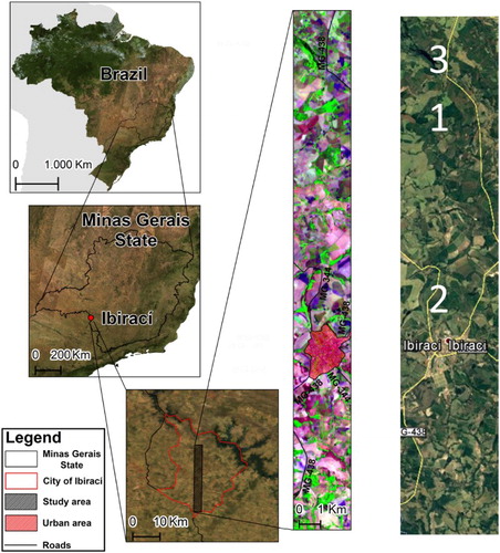
The mapping of fractional soil and vegetation components is carried out on EO-1 (low signal-to-noise) Hyperion imagery collected in the vicinity of Ibirací municipality (Figure 1), Minas Gerais, Brazil (20°27'41.65"S and 47°07'21.33"W, Datum WGS84). The area is characterized by elevations from 815 to 1120 m (above sea level) and undulating landforms with up to 20% slope (United States Geological Survey 2004). The soils in this region are weathering products of two geologic formations: Botucatu and Serra Geral (Heineck et al. 2003). These soils are categorized as iron-rich Latosols (180–360 g kg⁻¹ of iron oxides) found under tropical rainforest canopy, clay-rich Nitisols (>30% clay content) found in well-drained tropical savannah, and quartz-rich Arenosols (Amaral et al. 2005; IUSS Working Group 2007). According to the Köppen classification, the region’s climate is humid subtropical characterized by dry winter and temperate summer with rainfall of 1600–1900 mm year⁻¹ (Alvares et al. 2013). The natural vegetation occurring in this region belongs to the Cerrado biome, comprising a mixture of savannah and woodland ecosystem with gallery forests found in the wetter areas along stream corridors (Brazilian Institute of Geography and Statistics, 2004). The land use is characterized as a mixture of natural and cultivated pasture with agricultural hill crops and fragments of natural forest constrained mostly to areas near streams in the drainage system (Brazilian Institute of Geography and Statistics, 2010). The urban area of Ibirací (outlined) is located in the southern third of the study area.

Figure 1. Study area location and the portion of EO-1 Hyperion image used in the study (date of collection 2004/10/09; spectral bands centered in 1648.0, 823.0 and 661.0 nm in the RGB composition, respectively). Inset boxes represent priority regions of study at the pixel scale.

2.2. Field spectral signatures

The mapping of fractional landscape features from hyperspectral imagery requires training the unsupervised machine-learning network with signatures from relevant soil and vegetation components (Baldridge et al. 2009). To generalize this process, a set of field spectral signatures are chosen from soil (Ustin et al. 2009) and vegetation components (Vicente and de Souza Filho 2011) measured at independent sites but with tropical characteristics similar to the study area (Figure 2).

Figure 2. Independent field signatures of tropical soils and vegetation used in this study.

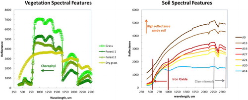
Some characteristics of vegetal components are the high variation of reflectance values associated with forest and grass transitions (Hartigan and Wong 1979), whereas characteristics of soil components include the presence of certain minerals (Serbin et al. 2009). For example, the chosen vegetation spectra characterize the main features, such as Forest1 (Aspen), Forest2 (Blackbrush), Grass (live), and GrassDry (dead), and diagnostic reflectance variations related to pigments in the visible region (400–700 nm), and generic biochemical compounds (e.g. starch, lignin), in the short-wave infrared (SWIR) region (1200–2500 nm) (Vicente et al. 2013). The main vegetation gradient is associated with longer wavelengths occurring in the transition between visible and near-infrared, the plateau characterized by broadleaf structures and canopy (800–1200 nm), and the water content in the leaf (above 2350 nm) (Ustin et al. 2009). These important spectral characteristics highlight the different stages of forest and grass as the main vegetation gradients.

The chosen soil spectra (A9, A13, A14, A16, A20, A21, and A27) characterize several important features. Firstly, the presence of iron oxides (A14) is typical of tropical Nitisols with the hematite appearing around 530 and 800 nm. Secondly, there is a gradual increase in soil reflectance toward longer wavelengths caused by an increase in particle size and presence of quartz (A9 and A13) characteristic of Arenosols. Thirdly, the feature occurring between 2100 and 2203 nm (SWIR) is attributed to the presence of hydroxyl (OH) associated with kaolinite clay (A16, A20, A21, and A27) typical of Latosols. The spectral signatures are resampled to the Hyperion spectral resolution (158 bands that range from 350 to 2100 nm) prior to processing described next.

2.3. Hyperion image

The Hyperion image is acquired over 242 spectral bands (SBs) at level 1Gst. Of the original image, 46 bands could not be calibrated because of the low spectral response, especially those on the early portion of the VNIR (355–426 nm) and late portion of the SWIR (2395–2405 nm). Another issue is in the overlapping of wavelengths between 852 and 1058 nm, covered by distinct spectroradiometers on VNIR and SWIR. For this reason, the study considered SBs 8–57 (436–926 nm) on VNIR and 79–224 (892–2406 nm) on SWIR, resulting into 196 calibrated bands (Jupp et al. 2004; Barry 2001). The final preprocessing step involved the elimination of atmospheric absorption bands: 120–132; 165–182; and 185–187 (Barry 2001). This sequence of preprocessing resulted in a total of 158 bands for use in classification (Vicente et al. 2013).

The original hyperspectral signals in the Hyperion image are gain corrected for atmospheric distortion using the fast line-of-sight atmospheric analysis of hypercubes (Bernstein et al. 2012). This process corrects wavelengths in the visible through near-infrared and SWIR regions, up to 3 µm. Next, the digital numbers are converted to reflectance values. For example, the effective signal gain of values in digital Numbers (DNs – Wm⁻² sr⁻¹ mM⁻¹), the data are scaled by 40; for bands in the VNIR region (bands: 1–70 and wavelengths: 0.400–1.000 µm) and by 80 for bands in the SWIR region (bands: 71–242, wavelengths: 0.900–2.500 µm), according to:(1) where L is the radiance value for band i (W m⁻² μm⁻¹ sr⁻¹) and DN_i is the digital number. These calibration coefficients are available in the Hyperion metadata. Gain values, G_i, are obtained by:(2) where R_i is commonly set equal to 0.025 and 0.0125 for VNIR and SWIR, respectively.

3. Methods

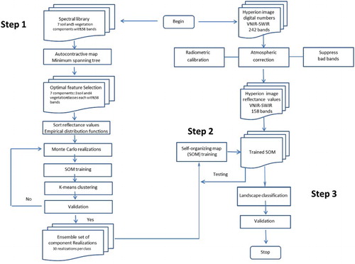
The proposed methodology is for mapping fractional soil and vegetation components from remote-sensing hyperspectral measurements. For that aim, there are three primary steps: (1) generate an unsupervised ensemble of optimal landscape training features, (2) train and validate an unsupervised classifier using the stochastic landscape features, and (3) perform estimation of landscape features in the hyperspectral reflectance image using a modified unsupervised classifier. A schematic outlining these steps and their associated tasks is presented in Figure 3.

Figure 3. Flowchart for the unsupervised landscape mapping of tropical soils and vegetation.

3.1. Unsupervised ensemble of optimal landscape training features

The generation of an ensemble of optimal landscape training features requires the following tasks: (1) select a set of field spectral signatures, (2) apply an ACM to quantify connectivity among SBs and landscape features, (3) apply a minimum spanning tree to organize connections and identify optimal groupings of landscape features, (4) perform stochastic simulation to generate landscape-component realizations, and (5) perform validation of the ensemble training set. Each of these tasks is briefly described in the following sections.

3.1.1. Field spectral signatures

Field spectral libraries provide measurements with reflectance information characterizing anticipated types of landscape features (e.g. soils and vegetation components) at the study site. Some characteristics of spectral libraries are the relatively large number (N ∼ 200) of SBs, and comparatively small number (N ∼ 10) of landscape-component signatures. In general, these characteristics present two challenges. First, the number spectral signatures (one for each component) are inadequate to train an unsupervised machine-learning network. Second, the reflectance amplitudes in spectral signatures are not sufficiently unique to differentiate one landscape feature to another. To overcome these challenges, the preprocessing of laboratory spectral signatures is undertaken to maximize information diversity by simulating the likely variation in signatures while taking advantage of the multiple SBs.

3.1.2. Autocontractive map

Application of the unsupervised ACM technique is used to identify the connectivity of laboratory SBs with landscape features (Buscema et al. 2010). The ACM architecture is characterized by three-layers: input layer (signals from the environment), hidden layer (where signals are modulated), and output layer (feedback to the environment). ACM mapping spatializes the correlation among variables by constructing a suitable embedding space where a visually transparent and cognitively natural notion, such as closeness among variables reflects accurately their associations. The learning algorithm may be summarized as follows (Buscema et al. 2010):

1. Signal transfer from the input into the hidden layer;(3) where m[s] are the units of the input layer (sensors) scaled between 0 and 1; m[h] are the units of the hidden layer, m[t] are the units of the output layer (system target), and v are the mono-dedicated connections, w are the connections (weights) between the hidden and output layer, C is a positive real number not lower than 1 (called the contraction parameter, often set C = √N), (n) subscript (omitted from the notation of the input layer units, as these remain constant at every cycle of processing), and N is the number of variables.

2. Adaptation of the connections vi(n) through the variation Δvi(n), which amounts to trapping the energy difference according to (1) is given by:(4) (5)

3. Signal transfer from the hidden into the output layer is given by:(6) (7)

4. Adaptation of the value of the connections w_i,j(n)through the variation Δw_i,j(n), which amounts, accordingly, to trapping the energy difference as to (5) is given by:(8) (9) (10)

where α is the learning coefficient of the ACM, and M is the number of records.

3.1.3. Minimum spanning tree

A minimum spanning tree is used to produce an undirected graph of SBs and their association to landscape features (Buscema et al. 2010). This representation is constructed by building a complex global graph of the complete pattern of variation from the ACM connectivity values. Moreover, this method fully exploits the topological meaningfulness of graph-theoretic representations in that actual paths connecting nodes (variables) represent the logical interdependence in explaining the variability in the data set. The minimum spanning tree is arrived at by finding an acyclic subset T of E that connects all of the vertices in the graph and whose total weight (i.e. the total distance) is minimized. The total weight is given by:(11) and(12) where T is the spanning tree, d_i,j is the distance edge, and MST is the T whose weighted sum of edges attains the minimum value.

To determine the MST of the undirected graph, each edge is weighted according to:(13) and(14) where w_ij is the matrix of connections, and is the joint probability of occurrence among variables (mutual information). Separations and groupings of graph connected spectral features constitute a means for selecting an optimal subset of signatures for use in the stochastic simulation step.

3.1.4. Stochastic simulation

Stochastic simulation is used to overcome the Hughes phenomenon (Medjahed et al. 2016) by providing a sufficient number of training signatures for unbiased classification of the optimally selected landscape features. Implementation of the simulation process is based on representativeness of the landscape empirical cumulative distribution functions (ECDFs) created from sorted spectral signatures. The Monte Carlo (MC) method is used to simulate each ECDF as a set of stochastic realizations (Tucker 1959). The MC simulation is based on the production of pseudo-random uniformly distributed values, a basic probabilistic distribution, required to simulate all other distributions where the produced numbers must be independent, that is, the number generated in one run does not influence the value of the next one. Efficiency of the stochastic simulation depends on knowledge about the problem; that is, the prior information that constrains the simulation, thus the importance of good probability distribution fitting with reliable parameters (Krajewski et al. 1991). Comparative statistical summaries of the fitted and simulated ECDF provide an objective measure for quality of the process. To ensure validity of the stochastic procedure, bias plots of the original and simulated spectral signatures can be plotted together with landscape realizations for each feature. Collectively these sets comprise the landscape ensemble used to train the unsupervised classifier.

3.2. Training and validation of the unsupervised classifier

3.2.1. Self-organizing map

The ensemble data set is used to train an unsupervised SOM. The SOM network is characterized by two-layer architecture: an input layer (signals from the environment) and an output layer (competitive feedback to the environment). The SOM uses a competitive learning algorithm to as a way of preserving the topology of multidimensional data in a lower dimensional space. The SOM learning algorithm may be summarized as follows (Kohonen 2001):

1. Generate initial values including weights, radius, learning parameter values

2. Select input vector from data set

3. Identify winning node, which is the closest node to the input vector using the Euclidean distance, D, metric:(15) where V is the input vector and W is the weight vector.

4. Identify the neighborhood with the given radius using a Gaussian function.(16) where σ₀ is the radius at t₀, λ is a time constant, and t is iteration.

5. Update the weights for the winning node and all the nodes in the same neighborhood.(17) (18) where W(t + 1) is weight for t = 1, L(t) is the learning rate at time t, V is the input vector. When update the weight values, exponential decay function is also used to decrease the learning rate. Learning rate value is decreased over time. The closer a node is to the winning node, the more its weights get altered (according to the same Gaussian function). Specifically, the learning rate is scaled by:(19) where the weights are adjusted using:(20)

6. Repeat steps 2–6 until the weight vectors reach a converged state.

The equations and issues regarding data gathering, normalization, and training are documented in Kohonen (2001).

3.2.1. Validation of the SOM network

Several visualization techniques have been developed to provide insight into quality of the trained SOM. One method used to define cluster boundaries in a SOM is the unified distance matrix, also called the U-matrix (Ultsch 2003). The U-matrix represents the relative closeness (in terms of Euclidean distance) between adjacent neurons on the SOM. This gives rise to a topographic analogy (valleys and ridges) in which the color differences represent class-boundaries, or samples belonging to different groups. Valleys, associated with low U values (cool colors), contain neurons whose weight vectors are close together, whereas high U values (warm colors) contain neurons whose weight vectors are distant from the weight vectors of its neighbors. One drawback of the U-matrix is that the average distance only is based on the final weight vectors; therefore, it does not take into account if the neuron represents one or more input vectors, or if it is far from most of the input vectors.

Mathematically, the u-matrix is described (Ultsch 2003) by:(21) where the values of elements u_ijli(j+1) u_ijl(i+1)j are the distances between the neighboring neurons M_ij and M_i(j+1) (M_ij and M_(i+1)j), respectively. The values of elements u_ij can be the average of neighboring elements of the u-matrix, for example, if u_ij has four neighbors, then u_ij = [u_i(j–1)ij + u_ijli(j+1) + u_(i–1)jlij + u_{(i+1)jli(j+1)}]/4. If the number of neighbors is smaller, the average is computed with a smaller number of elements. K-means clustering (Hartigan and Wong 1979) of the SOM neurons is conducted and superimposed on the U-matrix to assist in the association of landscape features.

3.3. Estimation using a modified classifier

Modification of the SOM classification algorithm allows for the simultaneous a-posteriori estimation of values associated with one or more variables (Wang 2003). To perform estimates, this study uses a scheme in which the values are arrived at iteratively based on simultaneous minimization of the quantization error, , and topographic error, , vectors. Computationally, the quantization error is the average distance between the data vectors and their neuron winners given by:(22)

In quantization error, , indicates how well neurons of the trained network adapt to the input vectors. Computationally, the topographic error is given by:(23)

The topographic error, , indicates how well the trained network keeps the topography of the data analyzed. If the neuron-winner of vector is closest to the neuron, that is, the distance from to it is the smallest one, then , otherwise . These are the same error vectors used in the SOM learning process to arrive at best matching unit vectors. In the estimation process, the values of interest are arrived at simultaneously for all variables across the hypersurface (Kalteh, Hjorth, Berndtsson 2008) with the initial starting values taken as the best matching unit vectors (Fessant and Midenet 2002; Wang 2003).

4. Results and discussion

4.1. Unsupervised ensemble of optimal landscape training features

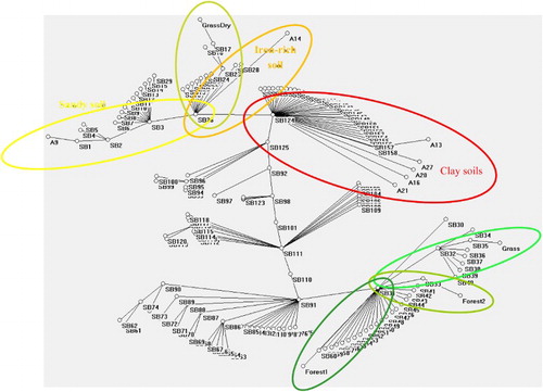
Application of the ACM and minimum spanning tree techniques to the spectral signatures identifies seven distinct landscape-component features (Figure 4). These landscape features are identified based on their selective connectivity along branches involving nodes defined by SBs. For example, the soil types A13, A16, A20, A21, and A27 are all connected to SB 124 (1386.65 nm). This finding suggests that there may not be sufficient spectral information for their individual classification. By contrast, the soil type A14 (iron oxide) is connected to SB26 (609.97 nm) and A9 (sandy loam) is connected along the branch from SB26 (609.97 nm) to SB3 (375.94 nm), SB3 (375.94 nm) to SB2 (375.94 nm), and SB2 (375.94 nm) to SB1 (355.59 nm). Similarly, the reflectance spectra for vegetation components can be characterized separately and therefore remain separate component classes. For example, dry grass (GrassDry) is connected along the path defined by branches occurring from nodes SB26 (609.97 nm) to SB25 (599.80 nm), and nodes SB25 (599.80 nm) to SB17 (518.39 nm), whereas live grass is connected along the branch defined between nodes SB 32 (671.02 nm) and SB35 (701.55 nm). The Forest1 component is defined by the SB31 (660.85 nm) node, whereas the Forest2 component is defined by branch connecting nodes SB 31 (660.85 nm) and SB33 (681.20 nm). These distinct groupings suggest that the ACM-MST approach may be used to tune hyperspectral sensor bands thereby minimizing the volume satellite data collected at field sites. These results further suggest that there is sufficient information content for application to image classification; however, the limited number of spectral signatures is inadequate to train a SOM.

Figure 4. Autocontractive results for tropical soils and vegetation presented as distances in a minimum spanning tree.

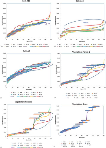
Application of the MC technique to the ECDFs for each of the landscape groupings provides realizations (N = 30) for each landscape feature (Figure 5). Each figure portrays the sorted signal reflectance as a function of spectral bins for each component. For each component, the SL equivalent signal is plotted together with random MC trials indicating the relative magnitude of uncertainty associated with the realizations. In general, the SL signal (purple) appears to fit with the stochastic simulations providing confidence in the ability to train a SOM network.

Figure 5. Comparison of signatures: Hyperion (0.95, 0.67, and 0.5), spectral library, and selected Monte Carlo (MC) realizations. Soil components: (a) clay-rich Latosols (A16), (b) iron-rich Nitisols (A14), (c) quartz-rich Arenosols (A9); Vegetation components: (d) Forest 1 (Aspen), (e) Forest 2 (Black), (f) grass, and (g) dry grass.

4.2. Training and validation of the unsupervised classifier

The component realizations are presented to three different map sizes for identifying an optimal network configuration: 14 × 10, 28 × 20, and 40 × 30. In each case, the SOM training proceeds first with a rough phase (20 iterations using a Gaussian neighborhood with an initial and final radius of 11 units and 3 units) and then fine phase (400 iterations using a Gaussian neighborhood with an initial and final radius of 3 units and 1 unit). The initial and final learning rates of 0.5 and 0.05 decay linearly down to 10^–5, and the Gaussian neighborhood function decreases exponentially (decay rate of 10^–3 iteration^–1) providing reasonable convergence. Following the training of these three networks, each corresponding SOM is used to independently classify the original SL signatures. In comparing the different SOM networks (Table 1), the 28 × 20 map size is chosen for independent reproducibility and processing speed. The corresponding k-means clusters overlying the U-matrix (Figure 6) reveal separation of the seven component classes for this map size thereby supporting it use for classification of the Hyperion imagery.

Figure 6. Clustering in the universal-distance matrix of SOM results. Individual clusters agree with the seven component types validating the stochastic SOM training process. Soil components: a) clay-rich Latosols (A16), (b) iron-rich Nitisols (A14), (c) quartz-rich Arenosols (A9); Vegetation components: (d) Forest 1 (Aspen), (e) Forest 2 (Blackbrush), (f) grass, and (g) dry grass. Individual clusters agree with the seven independent component types thereby validating the stochastic SOM training process.

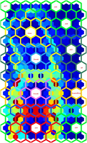
Table 1. Classification of landscape components by SOM and different network sizes.

		Soil			Vegetation
		A14	A16	A9	Forest1	Forest2	Grass	GrassDry	Map
	A14	0 . 93	0.01	0.00	0.02	0.03	0.00	0.00	14 × 10
	A16	0.02	0.95	0.00	0.00	0.00	0.00	0.03
Soil	A20	0.32	0.68	0.00	0.00	0.00	0.00	0.00
	A21	0.18	0.75	0.00	0.01	0.00	0.00	0.06
	A27	0.02	0.98	0.00	0.00	0.00	0.00	0.00
	A13	0.00	0.00	0.87	0.13	0.00	0.00	0.00
	A9	0.00	0.00	0.99	0.00	0.00	0.00	0.01
	Aspen	0.00	0.00	0.02	0.92	0.06	0.00	0.00
Vegetation	Black	0.03	0.00	0.00	0.12	0.85	0.00	0.00
	Grass	0.00	0.01	0.00	0.00	0.15	0.84	0.00
	GrassDry	0.00	0.21	0.00	0.00	0.00	0.01	0.78
	A14	0.98	0.02	0.00	0.00	0.00	0.00	0.00	28 × 20
	A16	0.00	0.95	0.00	0.00	0.00	0.02	0.03
Soil	A20	0.29	0.71	0.00	0.00	0.00	0.00	0.00
	A21	0.18	0.82	0.00	0.00	0.00	0.00	0.00
	A27	0.02	0.98	0.00	0.00	0.00	0.00	0.00
	A13	0.00	0.00	0.93	0.07	0.00	0.00	0.00
	A9	0.00	0.00	1.00	0.00	0.00	0.00	0.00
	Aspen	0.00	0.00	0.00	0.90	0.10	0.00	0.00
Vegetation	Black	0.02	0.00	0.00	0.00	0.98	0.00	0.00
	Grass	0.00	0.00	0.00	0.00	0.00	1.00	0.00
	GrassDry	0.00	0.17	0.00	0.00	0.00	0.00	0.83
	A14	0.99	0.00	0.00	0.00	0.01	0.00	0.00	42 × 30
	A16	0.00	0.96	0.00	0.00	0.00	0.00	0.03
Soil	A20	0.35	0.65	0.00	0.00	0.00	0.00	0.00
	A21	0.00	1.00	0.00	0.00	0.00	0.00	0.00
	A27	0.00	0.99	0.00	0.01	0.00	0.00	0.00
	A13	0.00	0.00	1.00	0.00	0.00	0.00	0.00
	A9	0.00	0.00	1.00	0.00	0.00	0.00	0.00
	Aspen	0.00	0.00	0.00	0.99	0.02	0.00	0.00
Vegetation	Black	0.00	0.00	0.00	0.00	1.00	0.00	0.00
	Grass	0.00	0.00	0.00	0.00	0.40	0.60	0.00
	GrassDry	0.01	0.00	0.00	0.00	0.00	0.01	0.98

Note: Soil components: clay-rich Latosols (A16), iron-rich Nitisols (A14), quartz-rich Arenosols (A9); Vegetation components: Forest 1 (Aspen), Forest 2 (Black), grass (live), and (g) dry grass (GrassDry). Classification results are from 1 (perfect correspondence) to 0 (no correspondence).

4.3. Estimation and validation of landscape feature components from hyperspectral imagery

A section (2.73 km × 24.5 km) of the original hyperspectral reflectance image comprising 11,761,204 reflectance values (158 bands × 91 pixels × 818 pixels) is presented to the trained SOM. This process resulted in classifying 74438 (30 m × 30 m) pixels with fractional variations of soil and vegetation features in about 15 s (Figure 5). Signatures from pixels classified with fractions >0.95 plot within the band of uncertainty in training signatures and are essentially coincident with the SL end-member signatures. In cases where pixels classify mixtures of fractional components <0.95, signatures deviate from the training set at wavelengths associated with other component types (blue oval). The mixing of sub-pixel landscape features is common in agricultural landscapes for various natural and anthropogenic reasons (Serbin et al. 2009).

A summary of estimated fractional landscape features is presented in Table 2. This table indicates the number of pixels, study area, and study area percentage for feature mixtures exceeding 0.1, 0.25, 0.5, 0.75, and 0.90. For example, the respective numbers of pixels comprising a 0.1 exceedance fraction (10%) or more of Latosol (A14), Nitosol (A16), Arenosol (A9), Aspen-like (Forest1), Blackberry-like (Forest2), live grass (Grass), and dead grass (GrassDry) are 37968 (34.2 km²), 56242 (50.6 km²), 809 (0.7 km²), 12140 (10.9 km²), 12949 (11.7 km²), 12282 (11.1 km²), and 3517 (3.2 km²). Other examples are presented for 0.25, 0.5, 0.75, and 0.9 exceedance values. In general, analysis of this table reveals that the clay-rich soils comprise the greatest proportion of study area. The next most prevalent soil feature is the iron-rich soils. The next most common landscape features are the forests with Blackberry-like trees about a factor two greater than Aspen-like trees. In contrast to other regions of the state, the quartz-rich soils appear to occupy an insignificant percentage (<1%) of the study area.

Table 2. A summary table of classified landscape features according to prescribed pixel exceedances.

Exceedance fraction	Landscape feature	Description type	Number pixels	Area (km^2)	Percent
0.1	a14	Latosol (iron-rich soil)	37968	34.17	51
	a16	Nitisol (clay-rich soil)	56242	50.62	76
	a9	Arenosol (quartz-rich soil)	809	0.73	1
	forest1	Aspen (tree)	12140	10.93	16
	forest2	Blackberry (tree)	12949	11.65	17
	grass	Grass (live)	12282	11.05	16
	grassdry	Grass (dead)	3517	3.17	5
0.25	a14	Latosol (iron-rich soil)	31695	28.53	43
	a16	Nitisol (clay-rich soil)	55795	50.22	75
	a9	Arenosol (quartz-rich soil)	746	0.67	1
	forest1	Aspen (tree)	3304	2.97	4
	forest2	Blackberry (tree)	5563	5.01	7
	grass	Grass (live)	1	0.00	0
	grassdry	Grass (dead)	10343	9.31	14
0.5	a14	Latosol (iron-rich soil)	11431	10.29	15
	a16	Nitisol (clay-rich soil)	53335	48.00	72
	a9	Arenosol (quartz-rich soil)	519	0.47	1
	forest1	Aspen (tree)	3268	2.94	4
	forest2	Blackberry (tree)	5563	5.01	7
	grass	Grass (live)	0	0.00	0
	grassdry	Grass (dead)	1400	1.26	2
0.75	a14	Latosol (iron-rich soil)	1367	1.23	2
	a16	Nitisol (clay-rich soil)	32466	29.22	44
	a9	Arenosol (quartz-rich soil)	408	0.37	1
	forest1	Aspen (tree)	0	0.00	0
	forest2	Blackberry (tree)	11	0.01	0
	grass	Grass (live)	0	0.00	0
	grassdry	Grass (dead)	1393	1.25	2
0.9	a14	Latosol (iron-rich soil)	723	0.65	1
	a16	Nitisol (clay-rich soil)	23640	21.28	32
	a9	Arenosol (quartz-rich soil)	0	0.00	0
	forest1	Aspen (tree)	0	0.00	0
	forest2	Blackberry (tree)	11	0.01	0
	grass	Grass (live)	0	0.00	0
	grassdry	Grass (dead)	376	0.34	1

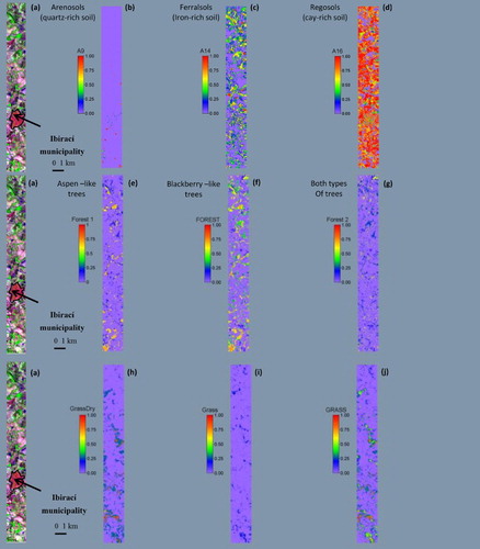
The unsupervised estimation of Hyperion landscape features results in mapping spatially heterogeneous soil, forest, and grass landscape components (Figure 7). It is noteworthy that both forest and soil features appear across the landscape as fractional gradients which provide an improvement over the traditional three-band (SBs centered in 1648.0 nm, 823.0 nm, and 661.0 nm in the red, green, blue composition, respectively; Figure 2) remote-sensing classification of soil, nonphotosynthetically active, and photosynthetically active vegetation. At any location, this improvement provides sub-pixel fractions of landscape features that sum to unity, as opposed to the presence or absence of a single feature. For this case, the most prevalent regional soil types appear to be Latosols (clay-rich), Nitisols (iron-rich) are intermediate, and Arenosols (quartz-rich) the least. The Aspen-like trees (Forest 1) are more prevalent than the Blackberry-like (Forest 2) deciduous trees. Based on these fractional maps, there appears to be more dry grass (GrassDry) than photosynthetically active grass (Grass).

Figure 7. Classification of fractional landscape components in the Hyperion scene: (a) OE-1 Hyperion image (red, green, blue bands centered at 1648.0 nm, 823.0 nm and 661.0 nm), (b) quartz-rich Arenosols (A9), (c) iron-rich Nitisols (A14), (d) clay-rich Latosols (A16), (e) Forest1 (Aspen-like trees), (f) Forest1 (Blackberry-like trees), (g) FOREST (all), (h) GrassDry (nonphotosynthetically active), (i) Grass (photosynthetically active), (j) GRASS (all).

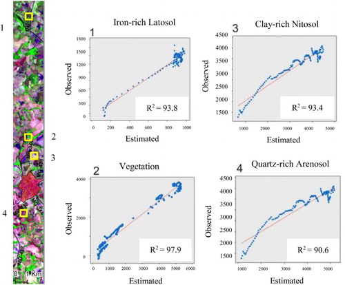
In general, the classified forests appear visually to correspond with existing drainages in the Google Satellite image as do iron-rich soils, whereas the clay-rich soils and grass appear on the intervening hills. These maps are independently corroborated (R² > 0.90) by comparing random soil samples to corresponding estimates of Latosols and Nitosols (Vicente et al. 2013). The soil spectra for different test areas along a gradient of sandy to clay soils are used as a simplified performance metric (Figure 8(a–c)). At each validation point, the spectral profile is extracted from the Hyperion image and compared to the estimated spectra. The regression plots show encouraging correspondence (R² > 0.90) supporting the use of field SL for mapping mixtures of Arenosols, Latosols, and Nitosols. Similar results are found for bias plots (R² > 0.98) of nonphotosynthetically active and photosynthetically active vegetation (Figure 8(d)).

Figure 8. Field verification: (a) Location of Hyperion soil test areas (CC R650/G548/B477) and (b) crossplots of observed versus estimated Hyperion spectra for soils: (1) iron-rich Latosol, (2) vegetation, (3) clay-rich Nitosol, (4) quarts-richArenosol.

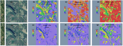
Locally expanded views of three study regions are provided to more closely evaluate the robustness of unsupervised mapping of soil and vegetation features across an agricultural landscape. In region 1 (Figure 9), the same general patterns exist among soil, forests, and grass as previously described. At this scale, however, it is possible to evaluate the fraction of landscape features that coexist as mixtures in pixels. Inspection of the forest classifications reveal that Forest 1 type trees appear to be riparian vegetation that is associated with the original drainage, whereas Forest 2 type trees also appear along and adjacent to the drainage. Those trees adjacent to the drainage are interpreted as part of managed and/or invasive species. In this figure, the workflow is able to map photosynthetically active (live) and nonphotosynthetically active (dead/dry) grass most notably in the northeast quadrant of the image. Similar findings are found in region 2 (Figure 10), but for this case the classification results for grass in the southeast quadrant appear to be compromised. Differences between the unsupervised map and Google image of grass in this quadrant may be attributed, in part, to differences in moisture content and season. In addition to moisture, shadows appear to confound the classification of vegetation. In region 3 (Figure 11), the large canyon occupying the northwest quadrant visually shows a shadow (low albedo) to the north (south facing side). Comparison of the classified Hyperion image with the Google image for this quadrant reveals that the pixel fractions appear to underestimate forest and overestimate soil fractions on the shadowed side of the valley. Lastly, row crops are evident in portions of the hill regions of the Google image but absent in the classified image. The absence of row crops in the classified image is to be expected because there were no related spectra introduced into the training process.

Figure 9. Mapping and verification of fractional landscape components in region 1 of the Hyperion scene: (a) Google Earth image, (b) quartz-rich Arenosols (A9), (c) iron-rich Nitisols (A14), (d) clay-rich Latosols (A16), (e) Forest1 (Aspen-like trees), (f) Forest1 (Blackberry-like trees), (g) FOREST (all), (h) GrassDry (nonphotosynthetically active), (i) Grass (photosynthetically active), (j) GRASS (all).

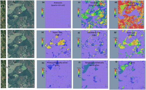
Figure 10. Mapping and verification of fractional landscape components in region 2 of the Hyperion scene: (a) Google Earth image, (b) quartz-rich Arenosols (A9), (c) iron-rich Nitisols (A14), (d) clay-rich Latosols (A16), (e) Forest1 (Aspen-like trees), (f) Forest1 (Blackberry-like trees), (g) FOREST (all), (h) GrassDry (nonphotosynthetically active), (i) Grass (photosynthetically active), (j) GRASS (all).

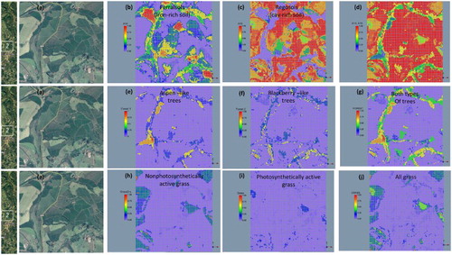
Figure 11. Mapping and verification of fractional landscape components in region 3 of the Hyperion scene: (a) Google Earth image, (b) quartz-rich Arenosols (A9), (c) iron-rich Nitisols (A14), (d) clay-rich Latosols (A16), (e) Forest1 (Aspen-like trees), (f) Forest1 (Blackberry-like trees), (g) FOREST (all).

It is important to emphasize that the unsupervised machine-learning workflow can be fully automated for future mapping of fractional landscape components. Specifically, the selection of most relevant bands is done by using the ACM; the MST is used to associate relevant SBs with landscape features; and the modified SOM is used to estimate fractional landscape components in the hyperspectral image. Given that the unsupervised classification workflow example relies on a limited number and independent set of spectral signatures, the proposed methodology has the potential to increase mapping accuracy and performance as additional local training sets are added.

5. Conclusions

The fractional mapping of tropical soils and vegetation features in Hyperion (low signal-to-noise) satellite imagery is possible using the proposed unsupervised machine-learning scheme and reflectance spectroscopy. The success of the classifier, however, is dependent on the optimal selection of signatures from a field SL, and the stochastic training of an unsupervised machine-learning algorithm. The optimal selection of spectral signatures is possible using an ACM and minimum spanning tree combination, and the classification is possible using a 2D SOM trained with an ensemble of landscape feature realizations. The trained SOM appears robust despite application without noise suppression and relatively large quantity of data contained in the imagery test scene (158 bands × 91 pixels × 818 pixels). The robustness as an estimator of landscape features is attributed to maintenance of multivariate and topologic relations along the processing sequence that otherwise would burden the processing time. The modified SOM appears to distinguish among variations in proportions of soils, trees, and grasses. For example, the mapping of fractional soil (for example, 0.5 exceedance for pixels: 75% clay-rich Nitisols; 15% iron-rich Latosols, and 1% quartz-rich Arenosols) and vegetation (for example, 0.5 exceedance for pixels: 4% Aspen-like trees, 7% Blackberry-like trees, 0% live grass, and 2% dead grass) mixtures. Some challenges are associated with the underestimation of fractional forest and overestimation of fractional soil where steep valley shadows exist, and the underrepresentation of classified grass in some areas of the Hyperion image. These preliminary results provide impetus for future hyperspectral studies involving airborne and satellite sensors with higher signal-to-noise and smaller footprints. We anticipate that as additional field data become available, the unsupervised mapping methodology will be increasingly effective for hyperspectral remote-sensing applications worldwide.

Acknowledgements

The author thanks Zara Rawlinson and Rogier Westerhoff of GNS Science and two anonymous reviewers for their detailed and constructive comments.

Disclosure statement

No potential conflict of interest was reported by the authors.

Additional information

Funding

This work was supported as part of the Smart Aquifer Characterization program funded by the Ministry of Business, Innovation and Employment.

References

- Alvares, C. A., J. L. Stape, P. C. Sentelhas, J. L. de M Gonçalves, and G. Sparovek. 2013. “Köppen’s Climate Classification Map for Brazil.” Meteorologische Zeitschrift 22 (6): 711–728. doi: 10.1127/0941-2948/2013/0507
- Amaral, F. C. S. do, R. P. de Oliveira, J. S. de Souza, M. L. D. Aglio, and C. E. Chaffin. 2005. Mapa de Solos do Estado de Minas Gerais [Soil Map of Minas Gerais State]. Rio De Janeiro: Embrapa Solos. Scale of the map 1:1.000.000.
- Awad, M. M. 2012. “A New Geometric Model for Clustering High-resolution Satellite Images.” International Journal of Remote Sensing 33 (18): 5819–5838. doi: 10.1080/01431161.2012.674228
- Baldridge, A. M., S. J. Hook, C. I. Grove, and G. Rivera. 2009. “The ASTER Spectral Library Version 2.0.” Remote Sensing of Environment 113: 711–715. doi: 10.1016/j.rse.2008.11.007
- Barry, P. 2001. EO-1/ Hyperion Science Data User’s Guide. Level 1_B. Redondo Beach: TRW Space, Defense & Information Systems, 60 pp.
- Bartholomeus, H., L. Kooistra, A. Stevens, M. van Leeuwen, B. van Wesemael, E. Ben-Dor, and B. Tychon. 2011. “Soil Organic Carbon Mapping of Partially Vegetated Agricultural Fields with Imaging Spectroscopy.” International Journal of Applied Earth Observation and Geoinformation 13: 81–88. doi: 10.1016/j.jag.2010.06.009
- Bernstein, L. S., X. Jin, B. Gregor, and S. Adler-Golden. 2012. “Quick Atmospheric Correction Code: Algorithm Description and Recent Upgrades.” Optical Engineering 51 (11): 111719-1–111719-11. doi: 10.1117/1.OE.51.11.111719
- Bruzzone, L., M. Chi, and M. Marconcini. 2006. “A Novel Transductive SVM for the Semisupervised Classification of Remote Sensing Images.” IEEE Transactions on Geoscience and Remote Sensing 44: 3363–3373. doi: 10.1109/TGRS.2006.877950
- Buscema, M., R. Petritoli, G. Pieri, and P. L. Sacco. 2010. AutoContractive Maps. Technical Paper 32. Rome: Semeion Institute.
- Camps-Valls, G., D. Tuia, L. Bruzzone, and J. Benediktsson. 2014. “Advances in Hyperspectral Image Classification.” IEEE Signal Processing Magazine 31 (1): 45–54. doi:10.1109/MSP.2013.2279179.
- Fauvel, M., J. A. Benediktsson, J. Chanussot, and J. R. Sveinsson. 2008. “Spectral and Spatial Classification of Hyperspectral Data using SVMs and Morphological Profiles.” IEEE Transactions on Geoscience and Remote Sensing 46 (11): 3804–3814. doi: 10.1109/TGRS.2008.922034
- Fessant, F., and S. Midenet. 2002. Self-Organizing Map for Data Imputation and Correction in Surveys. Neural Computing & Applications 10: 300–310. doi: 10.1007/s005210200002
- Gualtieri, J. A., and R. F. Cromp. 1999. “Support Vector Machines for Hyperspectral Remote Sensing Classification.” Proceedings of SPIE 3584: 221–232. doi: 10.1117/12.339824
- Guerschman, J. P., M. J. Hill, L. J. Renzullo, D. J. Barrett, A. L. Marks, and E. J. Botha. 2009. “Estimating Fractional Cover of Photosynthetic Vegetation, Non-Photosynthetic Vegetation and Bare Soil in the Australian Tropical Savanna Region Upscaling the EO-1 Hyperion and MODIS sensors.” Remote Sensing of Environment 113: 928–945. doi: 10.1016/j.rse.2009.01.006
- Hartigan, J. A., and M. A. Wong. 1979. “K-means Clustering Algorithm.” Applied Statistics 28: 100–108. doi: 10.2307/2346830
- Heineck, C. A., C. A. S. Leite, M. A. da Silva, and V. S. Vieira. 2003. Mapa geologico de Minas Gerais [Geological Map of Minas Gerais State]. Belo Horizonte: Brazilian Geological Service (CPRM)/Mining Company of Minas Gerais (COMIG). Map scale 1:1.000.000.
- Hentati, A., A. Kawamura, H. Amaguchi, and Y. Iseri. 2010. “Evaluation of Sedimentation Vulnerability at Small Hillside Reservoirs in the Semi-arid Region of Tunisia Using the Self-organizing Map.” Geomorphology 122: 56–64. doi: 10.1016/j.geomorph.2010.05.013
- Hewitson, B. C., and R. G. Crane. 2002. “Self-organizing Maps: Applications to Synoptic Climatology.” Climate Research 22 (1): 13–26. doi: 10.3354/cr022013
- Instituto Brasileiro de Geografia e Estatística (Brazilian Institute of Geography and Statistics). 2004. Mapa de Vegetacao do Brasil [Vegetation Map of Brazil]. Rio de Janeiro: IBGE. Map scale 1:5.000.000.
- Instituto Brasileiro de Geografia e Estatística (Brazilian Institute of Geography and Statistics). 2010. Mapa da Cobertura e Uso da Terra [Land Use and Cover Map]. Rio de Janeiro: IBGE. Map scale 1:5.000.000.
- IUSS Working Group WRB. 2007. World Reference Base for Soil Resources 2006, First Update 2007. World Soil Resources Reports No. 103. Rome: FAO.
- Iwashita, F., M. J. Friedel, G. F. Ribeiro, and S. J. Fraser. 2012. “Intelligent Estimation of Spatially Distributed Soil Physical Properties.” Geoderma 170: 1–10. doi: 10.1016/j.geoderma.2011.11.002
- Iwashita, F., M. J. Friedel, C. R. Souza Filho, and S. J. Fraser. 2011. “Hillslope Chemical Weathering Across Paraná State, Brazil: A Data Mining-GIS Hybrid Approach.” Geomorphology 132: 167–175. doi: 10.1016/j.geomorph.2011.05.006
- Jupp, D. L. B., B. Datt, J. Lovell, S. Campbell, and E. King. 2004. Discussions Around Hyperion Data: Background Notes for the Hyperion Data Users Workshop. Canberra: CSIRO, Office of Space Science and Applications Earth Observation Centre, 46 p.
- Kanevski, M., R. Parkin, A. Pozdnukhov, V. Timonin, M. Maignan, B. Yasalo, and S. Canu. 2004. “Environmental Data Mining and Modelling Based on Machine Learning Algorithms and Geostatistics.” Journal of Environmental Modelling and Software 19: 845–855. doi: 10.1016/j.envsoft.2003.03.004
- Kalteh, A. M., P. Hjorth, and R. Berndtsson. 2008. “Review of the Self-Organizing Map (SOM) Approach in Water Resources: Analysis, Modeling and Application.” Environmental Modelling & Software 23(7): 835–845. doi: 10.1016/j.envsoft.2007.10.001
- Keshava, N., and J. F. Mustard. 2002. “Spectral Unmixing.” IEEE Signal Processing Magazine 19: 44–57. doi: 10.1109/79.974727
- Kohonen, T. 2001. Self-organizing Maps. 3rd ext. ed. Springer Series in: Information Sciences, 30. Berlin: Springer, 253 p.
- Kohonen, T. 2013. “Essentials of the Self-organizing Map.” Neural Networks 37: 52–65. doi: 10.1016/j.neunet.2012.09.018
- Krajewski, W. F., V. Lakshmi, K. P. Georgakakos, and S. Jain. 1991. “A Monte Carlo Study of Rainfall Sampling Effect on a Distributed Catchment Model.” Water Resources Research 27: 119–128. doi: 10.1029/90WR01977
- Latif, A. B., R. Lecerf, G. Mercier, and L. Hubert-Moy. 2008. “Preprocessing of Low Resolution Time Series Contaminated by Clouds and Shadows.” IEEE Transactions on Geoscience and Remote Sensing 46 (7): 2083–2096. doi: 10.1109/TGRS.2008.916473
- Lohr, S. C., M. Grigorescu, J. J. Hodgkinson, M. E. Cox, and S. J. Fraser. 2010. “Iron Occurrence in Soils and Sediments of a Coastal Catchment: A Multivariate Approach Using Self Organising Maps.” Geoderma 156 (3–4): 253–266. doi: 10.1016/j.geoderma.2010.02.025
- Lu, P., L. Wang, Z. Niu, L. Li, and W. Zhang. 2013. “Prediction of Soil Properties Using Laboratory VIS–NIR Spectroscopy and Hyperion imagery.” Journal of Geochemical Exploration 132: 26–33. doi: 10.1016/j.gexplo.2013.04.003
- Medjahed, S. A., T. Ait Saadi, A. Benyettou, and M. Ouali. 2016. “A New Post-classification and Band Selection Frameworks for Hyperspectral Image Classification.” The Egyptian Journal of Remote Sensing and Space Science 19 (2): 163–173. doi:10.1016/j.ejrs.2016.09.003.
- Penn, B. S. 2005. “Using Self-organizing Maps to Visualize High-dimensional Data.” Computer & Geosciences 31: 531–544. doi: 10.1016/j.cageo.2004.10.009
- Plaza, A., J. A. Benediktsson, J. W. Boardman, J. Brazile, L. Bruzzone, G. Camps-Valls, J. Chanussot, et al. 2009. “Recent Advances in Techniques for Hyperspectral Image Processing.” Remote Sensing of Environment 113: S110–S122. doi:10.1016/j.rse.2007.07.028.
- Salimi, A., M. Ziaii, A. L. Amiri, M. H. Zadeh, S. Karimpouli, and M. Moradkhani. 2017. “Using a Feature Subset Selection Method and Support Vector Machine to Address Curse of Dimensionality and Redundancy in Hyperion Hyperspectral Data Classification.” The Egyptian Journal of Remote Sensing and Space Science. doi:10.1016/j.ejrs.2017.02.003.
- Serbin, G., G. S. T. Daughtry, E. R. Hunt Jr., J. B. Reeves III, and D. J. Brown. 2009. “Effects of Soil Composition and Mineralogy on Remote Sensing of Crop Residue Cover.” Remote Sensing of Environment 113: 224–238. doi: 10.1016/j.rse.2008.09.004
- Szidarovszky, F., L. Duckstein, and I. Bogardi. 1984. “Multiobjective Management of Mining Under Water Hazard by Game Theory.” European Journal of Operational Research 15: 251–258. doi: 10.1016/0377-2217(84)90215-7
- Tucker, H. G. 1959. “A Generalization of the Gilvenko-Cantelli Theorem.” The Annals of Mathematical Statistics 30 (3): 828–830. doi: 10.1214/aoms/1177706212
- Ultsch, A. 2003. “Maps for the Visualization of High-dimensional Data Spaces.” In Proceedings of WSOM ‘03, Fukuoka, Japan, pp. 225–236.
- United States Geological Service. 2004. “Shuttle Radar Topography Mission, 3 Arc Second Scene.” Global Land Cover Facility, University of Maryland, College Park, MD.
- Ustin, S. L., A. A. Gitelson, S. Jacquemoud, M. Schaepman, G. P. Asner, J. A. Gamon, and P. Zarco-Tejada. 2009. “Retrieval of Foliar Information about Plant Pigment Systems from High Resolution Spectroscopy.” Remote Sensing of Environment 113: S67–S77. doi: 10.1016/j.rse.2008.10.019
- Vicente, L. E., M. J. Friedel, F. Iwashita, and A. Koga-Vicente. 2013. “Mapeamento de Características de solos Tropicais Utilizando Self-Organizing Map Aplicado à Dados Hiperespectrais.” SBSR Brazilian Remote Sensing Symposium, April, Foz do Iguaçu, PR, Brazil.
- Vicente, L. E., and C. R. de Souza Filho. 2011. “Identification of Mineral Components in Tropical Soils Using Reflectance Spectroscopy and Advanced Spaceborne Thermal Emission and Reflection Radiometer (ASTER) data.” Remote Sensing of Environment 115 (8): 1824–1836. doi: 10.1016/j.rse.2011.02.023
- Wang, S. 2003. “Application of Self-Organising Maps for Data Mining with Incomplete Data Sets.” Neural Computing & Applications 12: 42–48. doi: 10.1007/s00521-003-0372-1