Geospatial web services pave new ways for server-based on-demand access and processing of Big Earth Data

ABSTRACT

Big Earth Data has experienced a considerable increase in volume in recent years due to improved sensing technologies and improvement of numerical-weather prediction models. The traditional geospatial data analysis workflow hinders the use of large volumes of geospatial data due to limited disc space and computing capacity. Geospatial web service technologies bring new opportunities to access large volumes of Big Earth Data via the Internet and to process them at server-side. Four practical examples are presented from the marine, climate, planetary and earth observation science communities to show how the standard interface Web Coverage Service and its processing extension can be integrated into the traditional geospatial data workflow. Web service technologies offer a time- and cost-effective way to access multi-dimensional data in a user-tailored format and allow for rapid application development or time-series extraction. Data transport is minimised and enhanced processing capabilities are offered. More research is required to investigate web service implementations in an operational mode and large data centres have to become more progressive towards the adoption of geo-data standard interfaces. At the same time, data users have to become aware of the advantages of web services and be trained how to benefit from them most.

KEYWORDS:

• Geospatial web services
• interoperability
• Big Earth Data
• open data
• Open Geospatial Consortium (OGC)

1. Introduction

Big Earth Data can comprise of long time-series of multi-dimensional geospatial data sets available from satellites, ground-based sensors or numerical-weather prediction (NWP) models (Overpeck et al. 2011; Yang et al. 2011; Vitolo et al. 2015 ; Dasgupta 2016). Advancements in sensing technologies and continuous improvements of NWP and climate models have improved their accuracy and spatio-temporal scope (Yang et al. 2011). A better accuracy and resolution of Big Earth Data are accompanied by a dramatic increase in data volume. The European Space Agency (ESA), for example, developed a new fleet of satellites, called the Sentinels, as part of the Copernicus programme, the European Union’s flagship programme for monitoring the Earth’s environment using satellite and in-situ observations. It is estimated that the data acquired by the Sentinel satellites per day will eventually represent a volume of 6.5 Terabytes (TB) (Copernicus Observer 2016). ESA projects the growth of its Earth Observation Archive to a volume of more than 50 Petabytes (PB) in 2022. Alone, the data from the Sentinels will account for more than two-thirds of it (Doherty 2016). The meteorological data archive of the European Centre for Medium-Range Weather Forecasts (ECMWF) has just gone beyond the 120 PB mark, thus being the world’s largest archive of meteorological data (ECMWF 2016a). In spring 2016, the production of the fifth generation of ECMWF atmospheric reanalyses of the global climate, ERA5, has started. It will be the first reanalysis produced as an operational service and is an ECMWF key contribution to the Copernicus Climate Change Service. The entire production of the ERA5 reanalysis will eventually have a data volume of 5 PB (Hersbach and Dee 2016). Within the next 10 years, ECMWF expects that the amount of data archived per day will multiply by a factor of 100 (ECMWF 2016b).

But large volumes of environmental data by themselves have no value. Most important is what is done with the data to create added-value products that eventually lead to informed decision-making. The Earth System is governed by global processes, which can now, with the current wealth of environmental data, be better understood and monitored. Based on global Landsat data, the Global Forest Watch (World Resources Institute 2017) project, for example, developed a web-based global forest monitoring system that shows areas of deforestation or reforestation within the last 12 years. A precise climate reanalysis data product, such as ERA-Interim (Dee et al. 2011), allows to monitor anomalies of various atmospheric parameters, for example, air temperature, over different time scales, such as the last month, the last year or even the last 30 years (ECMWF 2017a). Furthermore, climate reanalysis data are needed as reference climate information to predict anomalous or extreme weather events. More precise information on extreme weather helps countries to better prepare for it and to save lives. Another example are the high-resolution air quality products provided by the Copernicus Atmosphere Monitoring Service that help to monitor and predict the concentration on pollutants in the atmosphere. Public administrations can use this information to better inform society and give out health warnings (ECMWF 2017b). Thus, large volumes of environmental data give us the opportunity to move from analysing small study areas to the analysis of global inter-related processes, enabling an informed decision-making on a global scale.

Despite the opportunities a growing volume of Big Earth Data provides, it poses challenges to data organisations and data users alike. The capacity to acquire geographic information is currently greater than the capacity to manage, process and analyse the data (Dasgupta 2016; Guo, Wang, and Liang 2016 ). There is currently a gap between the vast amounts of geospatial data being generated and the technical capabilities of turning petabytes of raw data into information and knowledge. Data organisations are challenged to find new solutions to manage, store and archive these massive amounts of data. Current data dissemination systems face a heterogeneity problem. Service styles range from off-line ordering to real-time, on-demand downloading. However, only a few people have enough computing power and bandwidth to download and process multiple hundred GB of data (Wulder and Coops 2014). Insufficient storage space and processing power are the main challenges a data user faces. Due to limited capacities, data users are forced to decrease the problem. Thus, it is rather worked on case studies and proof of concepts based on smaller, more manageable subsets of data. Half of a data analyst’s time is used for data download, data harmonisation and data pre-processing, resulting in little time for data interpretation and turning large volumes of raw data into digestible information and knowledge (Giuliani, Dubois, and Lacroix 2013).

Data accessibility and the availability of adequate computing power remain a long-term bottleneck of geospatial sciences. Peng, Zhao, and Zhang (2011) label data accessibility and data reusability as the most important forces that drive current geospatial information research and technology.

One direction for large data centres is to offer web-based data access (Overpeck et al. 2011) and server-based geospatial data processing. Geospatial web service technologies have been created to facilitate the exchange of heterogeneous geospatial information and reveal new opportunities to disseminate data and to redefine the common geospatial data analysis workflow. Large volumes of multi-dimensional geospatial data can be accessed via the Internet and large parts of the processing can be executed at server-side. Thus, data duplication and data transport are minimised and the processing of and algorithm execution on large data-volumes are enabled (Wulder and Coops 2014). Geospatial web services are disruptive in multiple ways. Data providers are challenged to go beyond the mere provision of data and have to exploit strategies to also offer services for efficient processing and fast visualisation. Data users are prompted to explore the benefits of geospatial web services and to change their traditional data analysis workflow that contains downloading the data and executing the analysis only on smaller study areas.

This paper focuses on the interface standard Web Coverage Service (WCS) 2.0, its extension Web Coverage Processing Service (WCPS) and requirements of server implementations offering this standard. Practical examples from different Earth Science disciplines (Climate, Marine and Planetary) will highlight how this specific type of a geospatial web service may redefine the traditional way of accessing and processing large volumes of multi-dimensional geospatial data. The practical examples are linked to requirements a WCS and its server implementation has to fulfil, based on data user and data provider needs. As WCS is one of multiple geospatial web service options, the paper positions a WCS, its benefits and limitations, within the wider geospatial web service landscape. The paper is structured as follows: Section 2 gives an introduction to the wider geospatial web service landscape and introduces the architecture and system of the WCSs used for this paper’s use-cases. Section 3 reflects in detail on requirements that are set on geospatial web services in general and on a WCS in specific, from a data user’s as well as a data provider’s perspective. Section 4 presents four practical examples from different Earth Science Communities, showing how data access and processing with the help of a WCS benefit the traditional data analysis workflow. Section 5 puts the practical examples in context of current discussions in geospatial research and points out the pending challenges of geospatial web services and the interface standard WCS. The last section gives a short conclusion and a vision for the future geospatial data exploitation.

2. Web-based access to and processing of Big Earth Data

Traditional geospatial data dissemination systems put their focus on static information provision. Download services offer raw data via ftp servers or API’s. This kind of service has some major drawbacks: (i) data access is inflexible, as access to only static raw data (e.g. global data fields) is provided, (ii) it demands a lot of bandwidth resources, as more data are downloaded than users actually need and (iii) systems from different data providers do not follow common standards and are not interoperable with each other. The geospatial data analysis workflow in a traditional sense is to process the data on a local machine with a variety of different software. A tremendous amount of time is used for downloading, processing and harmonising data from different data providers (Zhao, Foerster, and Yue 2012). Zhao, Foerster, and Yue (2012) call this the ‘everything-locally-owned-and-operated’ paradigm that makes geospatial data analysis very time-consuming and expensive.

The geospatial industry and research landscape is changing from conducting spatial analyses locally within a desktop-based geographical information system (GIS) to accessing and processing geospatial data on the web (McKee, Reed, and Ramage 2011; Zhao et al. 2012).

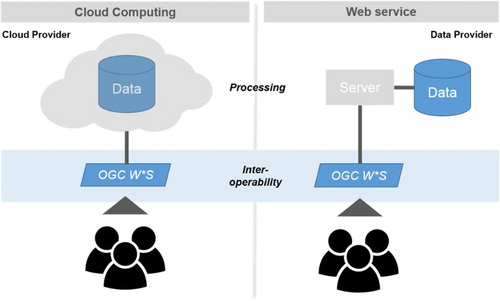
There are several options for data providers to offer web-based access to and processing of (geo-spatial) data. From a software architectural perspective, the concept of cloud computing or the concept of web services can be followed (Figure 1). In cloud computing, storage and computational facilities are no longer located on single computers, but distributed over remote servers operated by third-party providers, for example, Amazon Web Services or Google Cloud Platform (Schaeffer, Baranski, and Foerster 2010). In a cloud-based solution, a data provider puts the data to the cloud and it is the cloud provider’s responsibility to manage the data and to offer scalable, on-demand and cost-effective processing services to users. Google Earth Engine (2017) is an example of a cloud-based Software-as-a-Service solution to access and process geospatial data. Google Earth Engine offers access to petabytes of satellite, weather and climate data, which can directly be processed and analysed with custom processing scripts on the platform. Cloud computing may address the computationally challenging demands of the geospatial domain, but large data organisations need to carefully evaluate possible solutions.

Figure 1. Two different system architecture options to offer server-based data access and processing. Left: Cloud computing option, where data storage, management and processing are the responsibility of the cloud provider. Right: Web service option, where data storage, management and processing are the responsibility of the data provider. Optimally, in both cases, data users interact with interoperable standard interfaces, such as WCS.

The National Oceanic and Atmospheric Administration (NOAA) therefore initiated the Big Data Project that brings NOAA’s freely available data and subject matter expertise together with cloud provider’s infrastructure expertise (2017). Tangible benefits of the project are an easier access to NOAA’s data, while NOAA’s systems experience reduced loads and this leads to less costs for system maintenance and support in the long term. Current constraints are the availability and viability of cloud vendors and the dependency on one cloud provider. A further drawback is the current limited support of geospatial web standards of cloud platforms. Data and information cannot be easily shared or combined with other applications in an interoperable way. Large operational data centres, such as NOAA or ECMWF, further stress test cloud-based solutions with requirements to transfer massive data sets in real-time and complex multi-dimensional data sets (Bailey 2017). More future research and testing are required to understand the capabilities and limitations of cloud computing better.

The key principle of the web service concept is that data are managed and stored by the data owner/provider and data are accessible via the Internet in a standardised and interoperable way for the widest possible audience (Giuliani, Dubois, and Lacroix 2013). Web services, other than cloud computing, allow the connection of external data archives. Web services are based on a service-oriented-architecture approach. This means that service functionalities are offered by a set of independent, interoperable, distributed, loosely coupled software components (web services) that can be reused (Lopez-Pellicer et al. 2011; Peng, Zhao, and Zhang 2011; Giuliani, Dubois, and Lacroix 2013). Web services aim to provide users with a collection of functionalities needed for data access and sharing and are key enablers for providing interoperable access to spatial data (Giuliani, Dubois, and Lacroix 2013). Geospatial web services are a special kind of web service that provide access to heterogeneous geographic information on the Internet (Peng, Zhao, and Zhang 2011). THREDDS, GeoServer or rasdaman are common server solutions for geospatial web services (Vitolo et al. 2015).

Independent of the architectural choice to provide geospatial data access and processing, either via a cloud-based solution or via web services, key is the cross-platform interoperability that enables geospatial content sharing. The de facto standards for geospatial web service components are the standards developed by the Open Geospatial Consortium (OGC) (Lopez-Pellicer et al. 2011). OGC Web Services (OWSs) standards were developed to make geospatial data an integral part of web-based distributed computing and can also be part of the cloud.

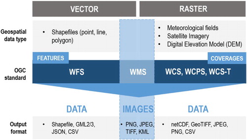
The OGC introduced various technical standard specifications that facilitate spatial data discovery, portrayal, download and processing (Figure 2). Catalog Service for the Web (OGC 2007) is used for data discovery, Web Feature Service (WFS) (OGC 2016) and WCS (OGC 2012) for retrieval of features and raster data, respectively, Web Processing Service (OGC 2015) and WCPS (OGC 2009; Baumann 2010) for data processing and analysis and Web Mapping Service (WMS) (OGC 2006) for data visualisation.

Figure 2. Overview of the OGC interface standards, which geospatial data type is offered by what standard and what output format can be expected.

OWS are based on XML (extensible markup language) standards and use HTTP for communication via the Internet (Kralidis 2007; Peng, Zhao, and Zhang 2011; Giuliani, Dubois, and Lacroix 2013).

View services, thus WMS, seem to be very well developed and widely accepted among different communities. Download services, however, are just emerging and only a few public WFS and even less WCSs are available (Giuliani, Dubois, and Lacroix 2013). The same applies for the availability of standardised processing services. The heterogeneity of raster data and formats and an often required re-engineering of current data dissemination systems hinder their frequent implementation.

However, if data users shall benefit from PBs of Earth data, geospatial data have to be made available beyond a simple view service. The WCS 2.0 specification by the OGC (2012) offers both functionalities, web-based access and server-based processing (Baumann 2010). The WCS specification ‘supports electronic retrieval of geospatial data as “coverages” – that is, digital geospatial information representing space/time-varying phenomena’. Hence, WCS is a standard data access protocol that defines and enables the web-based retrieval of multi-dimensional geospatial data sets (OGC 2012). It offers user-defined access to the geospatial data served from a web server and allows the user to ‘filter’ the data (Kralidis 2007). WCS supports slice and trim operations, where either the data dimension (slice) or the data extent (trim) is reduced. Unlike WMS, which returns spatial data as an image or ‘static map’, WCS returns data in its raw form, with its original semantics (OGC 2012). This allows for ad-hoc data processing and analysis or the building of web applications without prior data download.

The WCS core supports three main operations, which are submitted as HTTP requests to a specific URL:

• the GetCapabilities request returns an XML document with information to the service and data provider and an overview of all the coverages available on the web server.

• the DescribeCoverage request returns an XML document with metadata information of one specific coverage and

• the GetCoverage request returns a full coverage encoded as GeoTiff, XML or netCDF.

The WCS 2.0 core specification (OGC 2012) supports a processing extension, the WCPS (OGC 2009; Baumann 2010), and specifies an additional processing request:

• the ProcessCoverages request returns a coverage encoded in a specified format (e.g. netCDF, JSON or CSV) and allows for the processing and analysis of coverages.

WCPS allows the user to craft queries to be run on the data using a text-based query language, similar to SQL. Thus, the users are not only able to limit the data transfer to the area they are interested in, but also to take advantage of web-based, on-demand data processing. The WCPS extension can optionally be implemented by a WCS 2.0 server.

WCPS queries can be fairly straightforward and intuitive, as one example for climate reanalysis data shows:

&query = for c in (temp2m) return encode (c[Lat(53.0), Long(-1.0), ansi(“2012-01-01T00:00”: “2012-01-31T18:00”)] – 273.15, “csv”)

This WCPS query retrieves 6-hourly ERA-Interim (Dee et al. 2011) 2 m air temperature data for Reading, UK for January 2012. The temperature values are directly converted from Kelvin to degree Celsius. The WCPS syntax is quite powerful and can do quite complex calculations on the data. However, the more complex the processing request, the less intuitive the syntax becomes:

&query = for c in (temp2m) return encode((condense + over $x x(imageCrsDomain(c[Lat(-90:90), Long(-180:179.5),ansi(“2012-01-01T00:00”:“2012-01-31T18:00”)], ansi)) using c[ansi($x)]/124)-273.15, “csv”)

The query above takes advantage of a condenser function that is able to condense a 3D raster stack into its 2D average. The example aggregates global 2 m air temperature fields for January 2012 into one average field. Wagemann (2016) is a series of Jupyter notebooks that give a more detailed introduction to the two standard data access protocols WCS and WCPS.

3. Requirements for geospatial web services

WCSs are not as widely used as WMSs (Giuliani, Dubois, and Lacroix 2013). This is mainly due to the fact that multi-dimensional geospatial raster data differ in formats, coordinate systems and data models and semantics. There is still further research needed regarding the quality of service and performance and scalability of WCS implementations for a variety of different Earth Science data.

The H2020-funded EarthServer-2 project addresses this gap and sets up WCSs for different scientific domains: ocean science, earth observation, climate science and planetary science. The architectural setup follows the web services concept and bases on rasdaman (http://rasdaman.org/), an intelligent array-based server technology, in combination with the OGC standard protocol WCS. Four WCSs are exploring the possibilities and challenges of providing access to data sizes beyond 1 PB of 3D to 4D Earth Science Data:

• Marine Science Data Service (http://earthserver.pml.ac.uk/) is developed by the Plymouth Marine Laboratory (PML) and makes available multiple hundred terabytes of ocean colour data, produced by ESA’s climate change initiative (CCI). The service will further offer Sentinel-3 data once the data products are disseminated.

• Climate Science Data Service (http://earthserver.ecmwf.int/) is developed by the ECMWF and will provide access to multiple petabytes of ERA-Interim reanalysis data (Dee et al. 2011) stored in ECMWF’s archive. By serving data from the Meteorological and Archival System (MARS archive) via a web service in a standardised way, reanalysis data will become better accessible in a more tailored format to scientists and technical data users.

• Earth Observation (EO) Data Service (http://eodataservice.org/) is jointly developed by MEEO s.r.l. and the National Computing Infrastructure (NCI) Australia. The service will offer EO data from the Sentinel family, primarily data from Sentinel-2 satellites. NCI will eventually offer a WCS for multiple hundreds of terabytes of Landsat data.

• Planetary Science Data Service (http://planetserver.eu/) is developed by the Jacobs University Bremen and will provide access to tens of TB of data (topographic, multi- and hyperspectral) of the solar system bodies Mars, Mercury and Moon.

The data services for Marine Science and Climate Sciences aim more at technical data users, whereas the two latter, the data services for EO and for Planetary Science data, rather develop two data portals for respective end-users and decision-makers.

The diversity of the EarthServer-2 project partners is valuable to enhance the current geospatial web services, as all partners bring community-specific data user and data provider requirements for a WCS and its implementation (Table 1). The requirements have been gathered throughout the EarthServer-2 project and are based on interactions with community experts and general data users as well as feedback from workshop attendants.

Table 1. Overview of main requirements of a WCS from a data user and a data provider’s perspective.

Data user		Data provider
Type of data request	trim and slice operations	Support of data formats	community-specific formats such as GRIB and netCDF
Data encoding	image and data formats, such as csv or netCDF	Support of coordinate systems	e.g. CRS for planet Mars or Gaussian-Grid for meteorological data
Type of processing	mathematical equations, band calculation of EO data	Data semantics	proper representation of the data model
Metadata information	Retrieve associated axes information	Performance^a	Data request in time, independent of request type
		Scalability^a	Number of users
		Quality of Service^a	Monitoring of service, etc.

^aRequirements relate more to a WCS implementation rather than the standard WCS interface itself.

3.1. Data user requirements

We distinguish between two types of data users: (i) the technical data user, who has technical expertise in data handling and management and (ii) the end-user, who consumes information and needs pre-processed and value-added data to make decisions. End-users will not directly interact with a WCS and their requirements are often very domain-specific, this is why the collected user requirements primarily target the first user group, technical data users, who will most likely have an interest to use a WCS in a programmatic way. The requirements can be grouped in type of data request, data format, type of processing and metadata information.

Type of data request: operations on a data cube (multi-dimensional geospatial data sets) can be either trim (time-series retrieval) or slice (geographical subsets) operations. Users from most Earth Science communities are interested in performing both request types efficiently and fast. ECMWF data users, for example, are specifically interested in the point retrieval functionality, as ECMWF’s WebAPI (2015) allows efficient geographic sub-setting, but does not allow for efficient time-series retrieval.

Data encoding: The WCS 2.0 standard specification currently offers data outputs in image formats, such as PNG, Geotiff or JPEG, but also supports output data formats such as NetCDF, JSON and CSV. Especially, these formats are of interest for users, as large volumes of Big Earth Data usually need to be post-processed. CSV or JSON output encoding can directly be stored in a NumPy array, for example, and no data download as an intermediary step is required. NetCDF involves data download as an intermediary step, but is as well a popular data format to store array-oriented (raster) data from Earth Science disciplines (Unidata 2017).

Type of processing: different Earth Science disciplines require processing operations of different kind. The climate science community, for example, is interested in generating anomalies and averages of data over a certain period of time. For the EO community, WCPS is very useful to do band calculation, for example, to calculate on-demand the Normalised-Difference-Vegetation-Index (NDVI) of a satellite image.

Metadata: metadata are crucial to describe the data that are offered with a WCS. Here, a user needs all the information to understand the data, for example, data provider, geospatial and temporal resolution, parameter and its unit. The same applies for data requests. Besides the actual data array, a user is also interested in the accompanied axes information for each data value, as this facilitates further data processing and visualisation. The fulfilment of this requirement is still lacking at some server implementations. Axes information have to be manually created, based on the general geospatial metadata the service provides (resolution, minimum and maximum value of latitude/longitude information).

3.2. Data provider requirements

Data provider’s requirements rely on both the WCS standard interface and the WCS server implementation. They vary depending on the data organisation, for example, data may have to be disseminated in a 24/7 operational mode. The requirements for a WCS (standard interface and its implementation) from a data provider’s perspective can be grouped into data formats, coordinate systems, data semantics, service performance, scalability and Quality of Service.

Data formats: Big Earth Data are often multi-dimensional and complex. Common data formats are GeoTiff, NetCDF and for the meteorological community, GRIB. While expert users of a specific community are well trained to handle these data formats, users from other communities might struggle to use the data in their native format. The fact that users do not have to deal with native data formats and are able to directly access the data values is one of the main benefits of a WCPS. The support of native data formats, especially NetCDF and GRIB, as input data formats is critical for data providers, and a conversion of data should be avoided, as it is expensive and often leads to a loss in data quality.

Coordinate systems: scientific communities deal with different Coordinate Reference Systems (CRSs), beyond the standard WGS84 CRS. Correct mapping of data from the planet Mars, for example, requires a suitable CRS adapted to MARS (Marmo et al. 2016; Rossi et al. 2016). NWP (weather and climate) models often use a reduced Gaussian grid, which is regular in longitude and reduces the number of grid points along the shorter latitude lines near the poles (ECMWF 2017c).

Data semantics: data offered via a WCS have to be semantically correct. A data provider should be able to manually set up the data model, including multiple numbers of axes and the specification if axes have a continuous or discrete space. The meteorological community speaks of fields and data points, as forecasts are only valid for a specific point in space and time. The EO community works with pixels, where the spatial axes are treated as continuous information. Community-specific application profiles can be developed for the WCS specification. An application profile defines data structures and operations based on a community’s needs. It allows the retrieval of semantically correct coverages offered by a WCS server. The EO community developed a WCS EO Application Profile that describes the data structure of EO coverages. The meteorological community is currently developing a MetOcean Application Profile for WCS so meteorological data models can be described and retrieved in a semantically correct way.

Performance (time of response): the response time for data requested from a WCS should be minimal. If the aim is to build dynamic web applications based on a WCS, the response time should not exceed 10 s, as a user loses interest afterwards. A further challenge is to achieve a similar response time for different types of data requests, be it geographical sub-setting or point data retrieval. This is challenging, as these are two completely different requests to the data cube and challenges the internal structure of the data inside the database. Performance plays another major role, if an external archive is linked to a WCS implementation. The link with external archives is an orchestration of multiple different requests and every request has its own cost.

Scalability: this is an essential aspect for any data provider that considers offering a WCS implementation as an operational data service. Scalability in the context of web services is considered as being equally performant for 100,000 users than for ten users per day. Therefore, a WCS implementation has to withstand multiple requests simultaneously in an equally performant manner.

Quality of Service: major aspects of a quality geo-processing service are performance, scalability, reliability and availability. If the WCS is based on a third-party service, as is the case with the cloud computing and the web services solution, the data organisation is dependent on reliable updates and upgrades of the third-party software. This is especially crucial for data centres operating on a 24/7 operational basis, such as ECMWF or NOAA. Monitoring of service usage and limit of maximum data volume per request are further aspects that have to be considered.

4. Redefining the geospatial analysis workflow

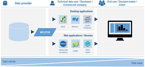
Retrieval and pre-processing of geospatial data are often the most time-consuming parts of the (geospatial) data analysis workflow and often take up to 50% of the total time (Giuliani, Dubois, and Lacroix 2013). Geospatial web services, Web Coverage (Processing) Service (WC(P)S) in particular, facilitate data access, retrieval and pre-processing and the analyst can dedicate more time to data analysis and interpretation. OWSs are the link between data provider and technical data users, developers or companies (Figure 3). If a data provider offers data access via a WCS, the technical data user (data analyst, scientist or developer) can easily integrate data access and processing into a processing routine. Be it building web applications with open-source web libraries such as NASA/ESA WebWorldWind or Open Layers or be it loading the data into a GIS for further spatial analysis.

Figure 3. Integration of a WC(P)S into the common geospatial data analysis workflow. The integration of WCPS requests can benefit technical data users to develop web or desktop applications for decision- and policy-makers.

Subsequently, four examples of how the traditional geospatial analysis workflow can benefit from a WCS 2.0 implementation are presented. We showcase how geospatial web services are beneficial for developing WebGIS systems and community-specific tools for Marine, Climate and Planetary Science. All examples provide information on the tool itself, the addressed community as well as the benefits the tools bring to the Earth Science community. Every example pictures also how the alternative workflow would look like. All examples are accompanied by either a weblink (WebGIS) or a dedicated Jupyter Notebook (Wagemann et al. 2016) for easy reproduction of the workflow and the examples presented. Table 2 provides a general overview of the four WCSs who are the basis for the four examples.

Table 2. Overview of the four WCS’s set-up in the course of EarthServer-2.

	Planetary science	EO science	Marine science	Climate science
Type of data	CRISM imagery	Landsat 8 (Europe) Landsat 5/7 (Italy)	ESA CCI Ocean colour	ERA-Interim climate reanalysis
Native data format	GeoTIFF	GeoTIFF	NetCDF	NetCDF, GRIB
WCS setup	rasdaman community	rasdaman enterprise^a	rasdaman enterprise^a	rasdaman enterprise^a
Type of data request	Complex band calculations of CRISM products	Band calculations, e.g. NDVI	Trim operation to retrieve point information	Trim and slice operations, mathematical aggregation
Use-case	WebGIS (4.1), RGB composition tool (4.4)	WebGIS (4.1)	Match-up tool (4.2)	Climate graph and monthly anomalies (4.3)

Note: all four service implementations use rasdaman as the server technology.

^aRasdaman enterprise offers the additional functionality to link external data archives with the server. This means that data stored and organised by another archive or database do not have to be duplicated. All web services that base on the rasdaman enterprise version want to benefit from this additional functionality.

4.1. WebGIS

In the course of the EarthServer-2 project, two enhanced WebGIS systems have been developed:

• the EO Data Service (http://eodataservice.org) for the EO community and

• PlanetServer (http://access.planetserver.org) for the Planetary Science community.

The EO Data Service offers access, analysis and visualisation of EO data for specific regions, for example, Landsat 8 over Europe, Landsat 5/7 over Italy and Austria and MODIS Level 2 and Level 3 products. The system is primarily used by scientists with strong subject matter expertise within their community, but with less knowledge about handling and analysing EO data.

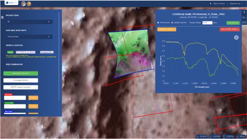
PlanetServer is primarily a tool to discover, visualise and analyse data from Planetary Science missions (Oosthoek et al. 2014; Marco Figuera et al. 2016) and is mainly used by the Planetary (Geo)Science community. Current users are mostly scientists involved in compositional studies of the surface of the planet Mars. Although for both systems the primary aim is research, the three-dimensional WebWorldWind client is suitable also for educational purposes.

The backend of both systems is based on rasdaman and offers the interoperability interface standard WCS 2.0 with its processing extension WCPS. The system of PlanetServer uses the open-source version of rasdaman, whereas the EO Data Service relies on the commercial version of rasdaman. This means, the data of PlanetServer is ingested into the rasdaman database, whereas the data of the EO Data Service are just linked with the server from an external archive.

Both systems offer advanced functionalities for their respective communities and showcase several user requirements. Both systems take advantage of the different types of data requests: (i) slice operation to retrieve a 2D image scene and (ii) a trim operation to retrieve a 1D vector of one pixel, for example, all data values for every time step or spectral data for every band of the satellite image. The two request types require two different format encodings. The slice operation requests an image format (e.g. PNG) to visualise the 2D image on-the-fly. The trim operation requests the data values as csv, which are then plotted with an appropriate plotting library. Both systems further take advantage of the processing extension WCPS and offer advanced spectral band operations of the satellite images. The EO data cube allows on-demand calculations of the NDVI for one respective pixel (Figure 4). PlanetServer allows to request spectral subsets of an image and to perform calculations on the returned values (Marco Figuera 2016). This allows for custom evaluation of spectral parameters (Figure 5).

Figure 4. A screenshot of the established WebGIS system EO Data Service. The service offers on-demand discovery, access, processing and retrieval of EO data from the Sentinel and Landsat satellites. The example shows the on-demand processing of a L8 image scene in order to retrieve NDVI information for a selected pixel.

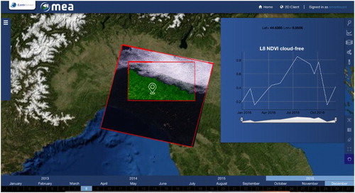
Figure 5. The PlanetServer web client. The left dock shows the projection and base maps selector and the RGB combinator. Spectral data plots from individual pixels can be visualised. The plot dock can load existing spectral data from laboratory samples for analysis.

The two WebGIS systems are examples of how an interactive and flexible visualisation and monitoring tool can be built based on an OGC standard interface WCS 2.0 implementation. Advanced processing functionalities can be offered if the processing extension WCPS is enabled.

4.2. Match-up tool for marine science applications

The marine science community uses Ocean colour satellite data to retrieve information on the concentration of chlorophyll. Chlorophyll concentration is a measure for the productivity of the oceans (Platt et al. 2008) and is one of the key variables monitored by commercial aquaculture groups. It further plays a key role in assessing bathing water quality and providing a basis for large areas of scientific ocean research. Ocean colour data from ESA’s CCI offers daily, weekly and monthly chlorophyll aggregates from 1997 to 2016. A monthly image with a spatial resolution of 4 km has a file size of ∼4 GB, resulting in multiple hundred GBs for the entire time period between 1997 and 2016.

The marine science remote sensing community often needs to compare remote sensed data values against in-situ data values that were collected at the same location. This comparison (match-up) process is used to validate remote sensed data or to tune regional algorithms (IOCCG 2012). The Marine Science Data Service developed a match-up tool to facilitate the comparison of in-situ measured data with remote sensed ocean colour data.

The service can be used through the web interface of the Marine Science Data Service (http://earthserver.pml.ac.uk/www/) or can be used from a custom python routine with the help of a predefined python code. The two options cater for different user types: users who prefer a simplified web interface and users who prefer to use the comparison tool as part of their customised python workflow.

The Marine Science Data Service is based on the rasdaman enterprise version and offers a WCS 2.0 standard interface with an enabled processing extension. The ESA CCI ocean colour data shall only be linked to the rasdaman server, as the data are already managed and stored in a different database hosted by PML.

The service takes advantage in particular of the trim data request, to retrieve data values of an individual latitude/longitude location. The service takes further advantage of the csv data encoding, as the real data values can be compared with measured data values.

The current alternative to the match-up tool based on a WCS would be to download the necessary data via a file transfer protocol (FTP) server. The user would then need to write custom code to extract the data values for one specific point location that matches the in-situ value. This approach has two drawbacks: (i) the required data transfer and (ii) the required processing capacities. As an example, even if a user is only interested in one chlorophyll value, an image of at least 4 GB has to be downloaded. With the help of a custom processing routine, the single value required could be retrieved. This process requires a lot of bandwidth, storage space and time, which can be avoided with a WCS. An example of how the match-up tool can be beneficial for scientists in Marine Sciences is provided as part of the Jupyter Notebooks developed by Wagemann et al. (2016). An alternative for the match-up tool via WCS could be a match-up service provided through a simple WebAPI, which also has to be developed by the data provider though.

4.3. WCPS benefits for climate science applications

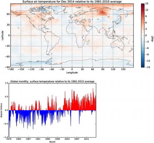
The climate science community analyses the state of the atmosphere over a long period of time. A climate scientist, for example, is interested in how the average surface temperature of one specific month, for example, December 2014, behaved compared to a long-term average for the month December or how the global monthly surface temperature developed relative to a normal period (generally, a period of 30 years, e.g. from 1981 to 2010) (see Figure 6).

Figure 6. Examples of information required for the climate science community. Above: Surface air temperature for December 2014 relative to the normal period (1981–2010) average. Below: Global monthly surface temperature relative to the 1981–2010 average from January 1979 to Dec 2014. Both graphs are based on ERA-interim reanalysis data.

Climate reanalysis data (e.g. ECMWF ERA-Interim) are currently the best representation of the historic state of the atmosphere (Dee et al. 2011). One ERA-Interim parameter (temporal/spatial resolution: 6-hourly, 0.5 deg lat/lon grid) from 1 January 1979 to 31 December 2014 has a volume of 27 GB.

For a climate graph, for example, time-series information for one specific location for two parameters, 2 m air temperature and total precipitation, would be required. The workflow would contain four distinctive steps. In a first step, the 6-hourly ERA-Interim values of 2 m air temperature need to be aggregated to monthly minimum, maximum and mean values. With one WCPS query, the 6-hourly values for 1 month can be retrieved and aggregated to either monthly min, max or mean. The same WCPS query can further convert the 2 m air temperature values from Kelvin to degree Celsius. The same process has to be repeated for the total precipitation parameter, with the exception that the monthly sums instead of averages are retrieved and the data values are converted from m to mm. In a third step, based on the time-series of monthly aggregated values, the average value of each month for 2 m air temperature and total precipitation is then calculated. In a final step, the average minimum, maximum and mean values for every month for both parameters are plotted.

Another example is shown in Figure 6. For the information there, global fields of 2 m air temperature for the period of 1 January 1979 to 31 December 2014 are required. For the top graph, monthly global fields of 2 m air temperature deviations relative to a normal period of 1981–2010 are needed. For the graph, a list that contains deviations of global surface temperature from the long-term average (1981–2010). The processing workflow would comprise five steps. The first step retrieves for every month the 6-hourly data values and aggregates them into monthly global means. In the same request, the unit of measurement is converted from Kelvin to degree Celsius. The second step retrieves for every month the global field and calculates for every data point a monthly average. The result is a raster stack of monthly global fields of 2 m air temperature from January 1979 to December 2014. In a third step, the long-term average for every month is calculated based on the normal period 1981–2010. The fourth step calculates then the monthly anomalies relative to the long-term average. The last step of the workflow is the visualisation of the results.

The Climate Science Data Service uses the rasdaman enterprise version, as the ERA-Interim data of ECMWF’s archive have a volume of more than 1 PB and ECMWF only wants to link its MARS archive with the rasdaman server. The data should optimally not be copied, but metadata should rather be registered. Data requested with a WCS request are then originating from the archive.

Data access via a WCS and processing via a WCPS brings multiple benefits for data users and data providers of climate data. First of all, with the help of a WCS request, time-series information for one specific latitude/longitude information can efficiently be retrieved without requiring a bulk download of multiple 2D fields. Second, with the mathematical condenser functions provided by a WCPS, a 3D raster stack can be condensed into its 2D average, minimum or maximum. Thirdly, through the SQL-like query language, mathematical operations can be applied. Data values of 2 m air temperature, for example, can be converted from Kelvin to degree Celsius on-the-fly.

One of the major benefits of a WCS for a meteorological data provider such as ECMWF is the independency of the data format from a data user perspective. Data users do not have to deal with complex and community-specific data formats, such as GRIB, and have direct access to the real data. This increases the data uptake from users outside the meteorological community to a large extent.

The alternative to the WC(P)S service is to use the WebAPI of ECMWF’s archive. The retrieval system is a very efficient system for 2D global fields or geographical subsets. For a time-series, however, a user is required to download a 2D field for every time step. The data can be retrieved either in netCDF or in GRIB format. Extensive processing would be the next step in order to retrieve the time-series information for one individual latitude/longitude information or to condense the data values, for example, 6-hourly values to a monthly average.

The Jupyter Notebooks created by Wagemann et al. (2016) contain in detail the two example workflows described above and showcase how WC(P)S data access and processing can be beneficial for climate science applications.

4.4. RGB composition tool for planetary science applications

One of the main research topics in planetary science is to characterise the surface mineralogy of different planetary bodies. A widely used technique for mineralogical characterisation is the use of hyperspectral imagery, which acquires a wider electromagnetic range, thus showing far more information than other techniques. Such images contain a large number of bands, which, combined in a particular sequence, allow highlighting of different mineralogical compositions.

Compact Reconnaissance Image Spectrometer for Mars (CRISM) imagery is one of the most important Mars data sets used by the planetary science community. The CRISM data set is formed by two sets of observations: the S observations ranging from 0.3 to 1 µm containing 107 bands and the L observations ranging from 1 to 4 µm containing 438 bands. In the example presented, only the L observations are used, as it is aimed to characterise the minerals kaolinites and Fe/Mg smectites that have a particular electromagnetic response within the L observation range.

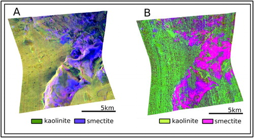
Viviano-Beck et al. (2014 ) and Pelkey et al. (2007 ) developed sets of band combinations so mineral characteristics can easier be retrieved for CRISM data. Both provide band math equations, called CRISM products, which help to highlight different types of minerals in a particular colour. The RGB channels of a CRISM image are assigned a specific CRISM product. As an example, in order to retrieve kaolinite and smectite based on the library developed by Pelkey et al. (2007), the red channel is assigned the CRISM product BD1900H, the green channel the CRISM product BD2200 and the blue channel the CRISM product D2300.

The Planetary Science Data Service developed a RGB composition tool for CRISM products that facilitates the creation of CRISM products and helps the planetary science community. The tool is written in Python and a user only requires the name of the image to be analysed and the name of the three CRISM products to be used (taken either from Pelkey et al. 2007 or Viviano-Beck et al. 2014). In principle, the tool helps a user to generate a WCPS query so she can retrieve the processed CRISM image with the selected combination as GeoTiff. The result can then be used for further analyses in a GIS system or a custom Python routine.

The tool takes advantage particularly of the processing extension WCPS. With one WCPS query, a user accesses one specific CRISM image, conducts band math calculations, applies an on-the-fly colour scheme and returns the final product as GeoTiff (Figure 7).

Figure 7. Comparison of different CRISM products for the image FRT0000A053. (A) uses R:BD1900H; G: BD2200; B: D2300 from Pelkey et al. (2007) and (B) uses R: BD1900 2; G: MIN2200; B: D2300 from Viviano-Beck et al. (2014).

Alternatives to the Python API presented include other open-source solutions developed in Python, IDL or C or proprietary solutions using ENVI. The RGB composition tool is open-source and available on GitHub (Halder and Marco Figuera 2016). The Jupyter Notebooks developed by Wagemann et al. (2016) contain as well an example workflow taking advantage of the RGB composition tool.

5. Discussion

The four distinct examples presented show how the OGC standard interface WCS 2.0 with its processing extension WCPS can provide web-based access to and server-based processing of large volumes of Big Earth Data in a standardised way. Examples highlight use cases of different communities, ranging from planetary sciences to EO community to climate and marine sciences. WC(P)S interfaces, together with their implementations, act as the direct link between the data provider and a technical data user, providing multiple benefits to the geospatial user community and service providers alike. Geospatial user communities benefit from web services as they offer on-demand access to information. A user only gets the information requested and does not need to download and manage the entire data set (Kralidis 2007). A web service implementation with a WCS interface offers time- and cost-efficient access to multi-dimensional data cubes, be it geographical sub-setting or time-series retrieval, as the example from the climate sciences showcased. As data are accessed on demand, a user does not have to take care of data set management and storage, shown by the examples from the marine and climate sciences. Data management tasks are delegated to the service provider and a user can ensure to receive the latest up-to-date data set (Kralidis 2007). As WC(P)S requests can easily be integrated into the geospatial workflow, applications and tools can be developed rapidly, as time-consuming data download, management and pre-processing can be neglected (Kralidis 2007). The presented WebGIS systems, EO Data Service and PlanetServer are examples for this. The standard status of WCS and WCPS is another benefit for data users. It allows users to reuse code to access and process data with WC(P)S for multiple applications or to combine data requests from multiple services within one processing routine. With a similar WCS request, a user can request data from the climate and the marine science service, for example. The overall goal, however, is to establish a web service federation. This eventually allows users to combine data access from different WCS providers and data processing in one single WCPS request. Users can neglect the physical location of the data repository and complicated customised solutions for data access. A web service federation of multiple WCS implementations will eventually lead to a true interoperability of decentralised data repositories of large data centres worldwide.

Service providers, on the other hand, benefit from reduced and bandwidth-saving data downloads. By providing data via a web service implementation together with a standardised WCS interface, eventually less data will be transported to a data user, which saves valuable bandwidth. A service provider further benefits from a potential increase in data uptake. Web services allow data access on demand without prior knowledge of community-specific data formats, for example, GRIB for meteorological data. This can lead to an increase in data uptake from users of other communities, as they can access and retrieve the data in a format they are most familiar with and do not have to learn how to deal with community-specific formats.

Despite the benefits of geospatial web services for data users and data providers, there are still some challenges to overcome. First, as the WCPS examples in Section 2 showed, the WCPS syntax is powerful, but can become quite complex. It further requires the learning of a new syntax. Both arguments can hinder users to fully take advantage of geospatial web services and the WCPS standard in particular. To ensure a wider usage of WCS and WCPS, tools have to be developed to make it easy for users to exploit the benefits. As part of the EarthServer-2 project, a python wrapper for WCPS is in development that in principle allows to connect to a WC(P)S server, and helps to craft a WCPS query and requests the query from the server. This wrapper will allow users to fully benefit from a WC(P)S service without learning a new syntax to use it. Second, data users have to be trained how to benefit from web services and the interoperability standards WCS and WCPS. As in agile software and web development, the training of users and collection of feedback should happen while web services are further evolving to also ensure their usability.

On data provider side, the implementation of geospatial web services is just one option to offer server-based data access and processing to users. As discussed in chapter 2, besides web services, a data provider could rather prefer a cloud-based solution at the backend. Both options bring advantages and disadvantages and data provider have to do a careful evaluation of what solution is best suited for their needs. Independent of the system architecture in the back, if data access and processing are offered via a cloud provider or via a dedicated web server within the data provider’s infrastructure, key are interoperability standards such as WCS and its extension WCPS. Despite the need for and benefits of interoperability of geospatial data from different communities and across country boundaries, the adoption of geo-standards at large and small data centres is not immediate. It would often require a re-engineering of current operational systems and organisations are still hesitant, often due to funding- and time-constraints, to go progressively towards offering full interoperable data services. The hesitation to change the system can also come from a lack of knowledge within data organisations about the benefits of these standards or not sufficient knowledge about data standards in general.

Technical challenges arise in the provision of a geospatial web service in an operational mode. Projects such as the Horizon2020-funded EarthServer-2 strongly contribute to the further development and dissemination of the interface standard WCS 2.0. User requirements for web services for different Earth Science communities are collected. At the same time, benchmarking studies are performed to get robust numbers of the scalability of WC(P)S implementations. The scalability is crucial, as the interface standard relies on a powerful backend, which is able to handle data access and processing requests in an efficient manner. If a web service is offered in an operational mode, the data provider has to ensure fast and reliable access to the service in a scalable manner. Scalable manner in this context means that the service has to withstand the concurrent access of massive numbers of users and user requests are handled efficiently. At the same time, more research is required regarding access control of web services and a limitation of the data volume per request. Additionally, for a WCS implementation costs for service maintenance and user support will arise.

A paradigm-shift is needed, not only on the side of data providers, but also on the side of users who use large volumes of geospatial data. Data users have to shift from the traditional geospatial data workflow where large volumes of data have been downloaded and replicated onto local machines towards a workflow with integrated web service standards for data access and processing, that does not require time-consuming data download anymore. Data providers have to be more progressive towards offering server-based data access and processing in a standardised and interoperable way.

6. Conclusion and outlook

A gap evolves between our ability to capture and acquire geospatial data and the ability to handle, manage, process and analyse it. Geospatial web service technologies, such as OGC WC(P)S, bring new opportunities to access large volumes of geospatial data via the Internet and to process them at server-side. This brings unforeseen opportunities for data users, as they are not restricted by available disc space and computing capacities of their local machines or organisations. Requests to an OGC WC(P)S can directly be integrated into existing processing routines, giving users more time to analyse and interpret data. They further allow for faster development of web applications. The overall goal are service federations that combine access and processing of data from different WCSs (from different data providers) into one single WCPS request.

Web service federations, besides geospatial web services offered by small and large data centres, are a promising solution for the future exploitation of Big Earth Data. They allow and allow to establish true interoperability of decentralised data repositories.

Acknowledgements

No direct benefit is given to the authors from the direct application of this research. The authors further want to acknowledge contributions of Anik Halder, Bang Pham Huu, Vlad Merticariu and Alex Dumitru for their support with web client development and rasdaman.

Disclosure statement

No potential conflict of interest was reported by the authors.

Additional information

Funding

This work was supported by the European Union’s Horizon 2020 Framework Programme research and innovation agreement [grant number 654367].

References

- Bailey, Andy. 2017. “The NOAA Big Data Project: Vision and Approach.” Presentation given at ECMWF Workshop of Meteorological Operational Systems, Reading, March 1-3. http://www.ecmwf.int/sites/default/files/elibrary/2017/17128-noaa-big-data-project-vision-and-approach.pdf.
- Baumann, Peter. 2010. “The OGC Web Coverage Processing Service (WCPS) Standard.” GeoInformatica 14 (4): 447–479. doi: 10.1007/s10707-009-0087-2
- Copernicus Observer. 2016. “Data Volume | Copernicus.” Copernicus Observer. Accessed 15 December 2016. http://newsletter.copernicus.eu/article/data-volume.
- Dasgupta, Arup. 2016. “The Continuum: Big Data, Cloud & Internet of Things.” Geospatial World 7 (1): 14–20.
- Dee, D., S. M. Uppala, A. J. Simmons, P. Berrisford, P. Poli, S. Kobayashi, U. Andrae, et al. 2011. “The ERA-Interim Reanalysis: Configuration and Performance of the Data Assimilation System.” Quarterly Journal of the Royal Meteorological Society 137 (656): 553–597. doi:10.1002/qj.828.
- Doherty, Mark. 2016. “Copernicus – A Game Changer in Earth Observation.” Presentation given at the United Nations / Austria Symposium on “Integrated Space Technology Applications for Climate Change”, Graz, September 12–14.
- ECMWF (European Centre for Medium-Range Weather Forecasts). 2015. “Access ECMWF Public Datasets – ECMWF WebAPI – ECMWF Confluence Wiki.” ECMWF. Accessed June 2017. https://software.ecmwf.int/wiki/display/WEBAPI/Access+ECMWF+Public+Datasets.
- ECMWF (European Centre for Medium-Range Weather Forecasts). 2016a. “Key Facts and Figures.” ECMWF. Accessed 15 December. http://www.ecmwf.int/en/about/media-centre/key-facts-and-figures.
- ECMWF (European Centre for Medium-Range Weather Forecasts). 2016b. “Drive to Boost Supercomputer Efficiency in Full Swing.” ECMWF, November 29. http://www.ecmwf.int/en/about/media-centre/news/2016/drive-boost-supercomputer-efficiency-full-swing.
- ECMWF (European Centre for Medium-Range Weather Forecasts). 2017a. “Average Surface Air Temperature Monthly Maps | Copernicus Climate Change Service.” ECMWF. Accessed 30 March. https://climate.copernicus.eu/resources/data-analysis/average-surface-air-temperature-analysis/.
- ECMWF (European Centre for Medium-Range Weather Forecasts). 2017b. “About CAMS | Copernicus Atmosphere Monitoring Service.” ECMWF. Accessed 30 March. https://atmosphere.copernicus.eu/about-cams.
- ECMWF (European Centre for Medium-Range Weather Forecasts). 2017c. “What is the Horizontal Resolution of the Data | ECMWF.” ECMWF. Accessed 11 July. https://www.ecmwf.int/en/what-horizontal-resolution-data.
- Giuliani, G., A. Dubois, and P. Lacroix. 2013. “Testing OGC Web Feature and Coverage Service Performance: Towards Efficient Delivery of Geospatial Data.” Journal of Spatial Information Science 7: 1–23. doi:10.5311/JOSIS.2013.7.112.
- Google. 2017. “Google Earth Engine.” Google. Accessed 29 March. https://earthengine.google.com/.
- Guo, H., L. Wang, and D. Liang. 2016. “Big Earth Data from Space: A New Engine for Earth Science.” Science Bulletin 61 (7): 505–513. doi:10.1007/s11434-016-1041-y.
- Halder, A., and R. Marco Figuera. 2016. “ PlanetServer Python API.” Zenodo. doi:10.5281/zenodo.204667.
- Hersbach, H., and D. Dee. 2016. “ERA5 Reanalysis is in Production.” ECMWF Newsletter 147: 7.
- IOCCG. 2012. “Mission Requirements for Future Ocean-Colour Sensors.” In Reports of the International Ocean-Colour Coordinating Group No. 13, edited by C. R. McClain and G. Meister, 1–103. Dartmouth: Author.
- Kralidis, A. T. 2007. “Geospatial Web Services: The Evolution of Geospatial Data Infrastructure.” In The Geospatial Web, edited by A. Scharl and K. Tochtermann, 223–228. London: Springer.
- Lopez-Pellicer, F. J., R. Bejar, A. J. Florczyk, P. R. Muro-Medrano, and F. J. Zarazaga-Soria. 2011. “A Review of the Implementation of OGC Web Services Across Europe.” International Journal of Spatial Infrastructures Research 6: 168–186. doi:10.2902/1725-0463.2011.06.art8.
- Marco Figuera, R., 2016. “PlanetServer Web Client.” Zenodo. doi:10.5281/zenodo.200371.
- Marco Figuera, R., B. Pham Huu, A. P. Rossi, M. Minin, J. Flahaut, and A. Halder. 2016. “Online Characterization of Planetary Surfaces: PlanetServer-2, an Open-Source Web Service.” Planetary and Space Science. ( Submitted Publication).
- Marmo, C., T. Hare, S. Erard, B. Cecconi, F. Costard, F. Schmidt, and A. P. Rossi. 2016. “FITS Format for Planetary Surfaces: Bridging the Gap Between Fits Word Coordinate Systems and Geographical Information Systems.” Paper Presented at the 47th lunar and planetary science conference, Texas, March 21–25.
- McKee, L., C. Reed, and S. Ramage. 2011. “OGC Standards and Cloud Computing.” OGC White Paper. Accessed 29 March. http://www.opengeospatial.org/docs/whitepapers.
- NOAA (National Oceanic and Atmospheric Administration). 2017. “Big Data Project.” NOAA. Accessed 29 March 2017. http://www.noaa.gov/big-data-project.
- OGC (Open Geospatial Consortium). 2006. “OpenGIS Web Map Server Implementation Specification: OGC Document 06-042.” OGC. Accessed 15 December. http://www.opengeospatial.org/standards/wms.
- OGC (Open Geospatial Consortium). 2007. “OpenGIS Catalogue Services Specification: OGC Document 07-006r1.” OGC. Accessed 15 December. http://www.opengeospatial.org/standards/cat.
- OGC (Open Geospatial Consortium). 2009. “Web Coverage Processing Service (WCPS) Language Interface Standard: OGC Document 08-068r2.” Accessed 15 December. http://www.opengeospatial.org/standards/wcps.
- OGC (Open Geospatial Consortium). 2012. “OGC WCS 2.0 Interface Standard: OGC Document 09-110r4.” OGC. Accessed 15 December. http://www.opengeospatial.org/standards/wcs.
- OGC (Open Geospatial Consortium). 2015. “OGC WPS 2.0 Interface Standard: OGC Document 14-065.” OGC. Accessed December 15. http://docs.opengeospatial.org/is/14-065/14-065.html.
- OGC (Open Geospatial Consortium). 2016. “Web Feature Service Implementation Specification: OGC Document 04-094r1.” OGC. Accessed 15 December. http://docs.opengeospatial.org/is/04-094r1/04-094r1.html.
- Oosthoek, J. H. P., J. Flahaut, A. P. Rossi, P. Baumann, D. Misev, P. Campalani, and V. Unnithan. 2014. “PlanetServer: Innovative Approaches for the Online Analysis of Hyperspectral Satellite Data from Mars.” Advances in Space Research 53 (12): 1858–1871. doi: 10.1016/j.asr.2013.07.002
- Overpeck, J. T., G. A. Meehl, S. Bony, and D. R. Easterling. 2011. “Climate Data Challenges in the 21st Century.” Science 331: 700–702. doi:10.1126/science.1197869.
- Pelkey, S. M., J. F. Mustard, S. Murchie, R. T. Clancy, M. Wolff, M. Smith, R. E. Milliken, et al. 2007. “CRISM Multispectral Summary Products: Parameterizing Mineral Diversity on Mars from Reflectance”. Journal of Geophysical Research E: Planets 112 (8): E08S14. doi:10.1029/2006JE002831.
- Peng, Z., T. Zhao, and C. Zhang. 2011. “Geospatial Semantic Web Services: A Case for Transit Trip Planning Systems.” In Geospatial Web Services: Advances in Information Interoperability, edited by P. Zhao and L. Di, 169–188. New York: IGI Global.
- Platt, T., N. Hoepffner, V. Stuart, and C. Browb. 2008. “Why Ocean Colour? The Societal Benefits of Ocean-Colour Technology.” Reports of the International Ocean-Colour Coordinating Group No. 7, IOCCG, Dartmouth Canada.
- Rossi, A.P., T. Hare, P. Baumann, D. Misev, C. Marmo, S. Erard, B. Cecconi, and R. Marco Figuera. 2016. “Planetary Coordinate Reference Systems for OGC Web Services.” Paper Presented at the 47th Lunar And Planetary Science Conference, Texas, March 21–25.
- Schaeffer, B., B. Baranski, and T. Foerster. 2010. “Towards Spatial Data Infrastructures in the Clouds.” In Geospatial Thinking: Lecture Notes in Geoinformation and Cartography, edited by M. Painho, M. Santos, and H. Pundt, 399–418. Berlin: Springer.
- Unidata. 2017. “Unidata | NetCDF.” Unidata. Accessed June 13. https://www.unidata.ucar.edu/software/netcdf/.
- Vitolo, C., Y. Elkhatib, D. Reusser, C. J. A. Macleod, and W. Buytaert. 2015. “Web Technologies for Environmental Big Data.” Environmental Modelling & Software 63: 185–198. doi:10.1016/j.envsoft.2014.10.007.
- Viviano-Beck, C.-E., F. P. Seelos, S. L. Murchie, E. G. Kahn, K. D. Seelos, H. W. Taylor, K. Taylor, et al. 2014. “Revised CRISM Spectral Parameters and Summary Products Based on the Currently Detected Mineral Diversity on Mars.” Journal of Geophysical Research: Planets 119 (6): 1403–1431. doi:10.1002/2014JE004627.
- Wagemann, J. 2016. “OGC Web Coverage Service Tutorial.” Zenodo. doi:10.5281/zenodo.205442.
- Wagemann, J., O. Clements, R. Marco Figuera, S. Mantovani and A. P. Rossi. 2016. “Geospatial Workflow with WCPS.” Zenodo. doi:10.5281/zenodo.202375.
- World Resources Institute. 2017. “Monitoring Forests in Near Real Time | Global Forest Watch.” World Resources Institute. Accessed 30 March. http://www.globalforestwatch.org/.
- Wulder, M. A., and N. C. Coops. 2014. “Satellites: Make Earth Observations Open Access.” Nature 513: 30–31. doi:10.1038/513030a.
- Yang, C., M. Goodchild, Q. Huang, D. Nebert, R. Raskin, Y. Xu, M. Bambacus, and D. Fay. 2011. “Spatial Cloud Computing: how can the Geospatial Sciences use and Help Shape Cloud Computing?” International Journal of Digital Earth 4 (4): 305–329. doi:10.1080/17538947.2011.587547.
- Zhao, P. L. Di, W. Han, and X. Li. 2012. “Building a Web-Services Based Geospatial Online Analysis System.” IEEE Journal of Selected Topics in Applied Earth Observations and Remote Sensing 5(6): 1780–1792. doi:10.1109/JSTARS.2012.2197372.
- Zhao, P., T. Foerster, and P. Yue. 2012. “The Geoprocessing Web.” Computers and Geosciences 47: 3–12. doi:10.1016/j.cageo.2012.04.021.