Modeling three-dimensional forest structures to drive canopy radiative transfer simulations of bidirectional reflectance factor

ABSTRACT

Three-dimensional (3-D) Monte Carlo-based radiative transfer (MCRT) models are usually used for benchmarking in intercomparisons of the canopy radiative transfer (RT) simulations. However, the 3-D MCRT models are rarely applied to develop remote sensing algorithms to estimate essential climate variables of forests, due mainly to the difficulties in obtaining realistic stand structures for different forest biomes over regional to global scales. Fortunately, some of important tree structure parameters such as canopy height and tree density distribution have been available globally. This enables to run the intermediate complexities of the 3-D MCRT models. We consequently developed a statistical approach to generate forest structures with intermediate complexities depending on the inputs of canopy height and tree density. It aims at facilitating applications of the 3-D MCRT models to develop remote sensing retrieval algorithms. The proposed approach was evaluated using field measurements of two boreal forest stands at Estonia and USA, respectively. Results demonstrated that the simulations of bidirectional reflectance factor (BRF) based on the measured forest structures agreed well with the BRF based on the generated structures from the proposed approach with the root mean square error (RMSE) and relative RMSE (rRMSE) ranging from 0.002 to 0.006 and from 0.7% to 19.8%, respectively. Comparison of the computed BRF with corresponding MODIS reflectance data yielded RMSE and rRMSE lower than 0.03 and 20%, respectively. Although the results from the current study are limited in two boreal forest stands, our approach has the potential to generate stand structures for different forest biomes.

KEYWORDS:

• Bidirectional reflectance factor
• remote sensing
• forest structure
• radiative transfer model

View correction statement:

Corrigendum

1. Introduction

Satellite estimation of essential climate variables (ECVs) of forests, like leaf area index (LAI), fraction of absorbed photosynthetically active radiation and Albedo, is crucial for understanding their roles in global carbon, water, and energy budgets (GCOS 2011). The satellite estimation algorithms of the ECVs rely on implementing the inversion of certain forward models against Earth observation (EO) data sets. The forward models could be empirical, analytical, or based on the mathematical expression of the physical theories underpinning the radiation transfer. Given accurate and reliable information from the EO data, the quality of these models is essential for the estimation accuracies of ECVs.

In recent decades, a wide variety of physically based forward models has been proposed to simulate the radiation properties of forests, such as the bidirectional reflectance factor (BRF) and hemispherical fluxes. The models include radiative transfer (RT) models that use purely analytical formulations (e.g. 2-Stream; Pinty et al. 2006), or ray-tracing methods based on Monte Carlo (MC) techniques (e.g. FLIGHT, North 1996; Forest Light Environmental Simulator (FLiES), Kobayashi and Iwabuchi 2008), as well as a large number of hybrid models based on the combination of one or several RT models, with numerical, stochastic, and/or geometric optical (GO) approaches (e.g. 4SAIL2, Verhoef and Bach 2003; 5SCALE, Leblanc and Chen 2000 ). Among these models, the Monte Carlo-based radiative transfer (MCRT) models yielded a model agreement around 1% on average, thus were used for benchmarking in intercomparisons of canopy RT simulations. For example, they were taken as the ‘surrogate truth’ in the third and fourth Radiation Transfer Model Intercomparison exercises (Widlowski et al. 2007, 2013). However, the MCRT models are rarely applied to develop inversion algorithms for estimating ECVs of forests, due mainly to the difficulties in obtaining realistic stand structures for a variety of forest biomes, as well as the requirement of extensive amount of CPU time.

The forest structure parameters – including the locations and architectures of individual trees – must be explicitly assigned as a prerequisite for running the MCRT models (Kobayashi et al. 2010; Morton et al. 2014). Although several previous studies on global retrieval of LAI have provided some concise descriptions of the structural parameters for each vegetation biome (e.g. Knyazikhin et al. 1998; Deng et al. 2006), we cannot regenerate the forest structure parameters for driving MCRT models from their descriptions. This situation has largely hindered third-party implementations and validations within the research communities. On the other hand, the forest structure parameters can sometimes be derived from some tree censuses, which are usually expensive and require a lot of manpower. For example, Kuusk et al. (2012) collected and released the full forest structure data sets for RT simulations based on extensive field measurements undertaken in Järvselja, Estonia. However, there are still several limitations when applying data sets of tree census to drive the MCRT models: first, the investigation parameters in traditional forest inventories cannot always meet the requirements for running RT models; second, the representativeness of inventory sites with respect to various forests is questionable; last, the limited frequency of field investigations cannot guarantee adequate monitoring of the forest dynamics resulting from growth and/or disturbances. Ground-based Light Detection and Ranging (LiDAR) is another effective way to collect detailed forest structure parameters for driving the MCRT models. However, its data sets are currently only available at some limited test sites (e.g. Lovell et al. 2003; Yao et al. 2011).

An alternative means is the modeling of three-dimensional (3-D) forest structures. For example, Disney et al. (2006) developed a 3-D model of a conifer forest canopy located in Thetford Forest, UK (hereafter denoted as Disney-model). In this model, the tree locations were randomly selected within a domain, and the canopy architectures were determined using the so-called Treegrow model (Leersnijder 1992). The model outputs were used to drive optical and microwave simulations of canopy scattering, and the simulated results agreed well with airborne hyperspectral reflectance data and airborne synthetic aperture radar backscatter data, respectively. Although the Disney-model can yield very detailed 3-D forest structures, it is a hard task to apply it to a variety of forest biomes over regional to global scales because more than 40 parameters need to be empirically tuned according to the forest characteristics. Fortunately, some of important tree structure parameters such as forest canopy height and tree density (TD) distribution have been available globally (Simard et al. 2011; Crowther et al. 2015). This enables to run the intermediate complexities of the 3-D MCRT models over the regions beyond the stand scale when appropriate scheme is available to compile these parameters into acceptable forest stand structures.

Consequently, the objectives of this study were (1) to develop a simple and effective approach for generating 3-D forest structure with an intermediate complexity (compared to the Disney-model) to drive the MCRT simulations and (2) to validate its performance at two boreal forest stands at Estonia and USA. Its goal is to yield agreements between the simulations of RT models using the generated and field measured forest structure parameters satisfying the theoretical accuracy requirement of atmospheric correction algorithm of MODIS reflectance product for each band (Vermote and Vermeulen, 1999). That is, the relative errors for red, near-infrared (NIR), and shortwave-infrared (SWIR) bands are lower than 30%, 6%, and 8%, respectively. In the proposed approach, the heights and locations of individual trees were determined by adopting the corresponding statistical distribution models; and the tree architectures are determined according to the allometric equations.

2. Data collection

2.1. Field data

The first forest site was located at Järvselja Training and Experimental Forestry District (27.268°E, 58.324°N), Järvselja, Estonia (Kuusk et al. 2012). A square plot of 100 × 100 m was marked within the study site, and the structural parameters were measured in summer 2007. The trees with diameter at breast height (DBH) larger than 4 cm were tallied, and their DBHs were determined by a Masser Racal electoral caliper. The tree locations were measured using a DTM-332 Total Station. Allometric equations of tree height (TH) and the crown dimensions were constructed using a group of 45 tree samples. A non-linear least squares regression method was used to estimate parameter values for the allometric models of TH, crown length (CL), and crown radius (CR). Then the constructed estimation equations were applied to all the tallied trees. In the application to our proposed approach, the allometric equations were re-calibrated using TH as the independent factor, as summarized in Table 1. Moreover, the true LAI value of 2.21 was derived by a LAI-2000 plant canopy analyzer. Detailed information regarding the forest stand and landscape data set can be obtained from Kuusk et al. (2012).

Table 1. Estimation models of DBH, CL, and CR based on TH for the Järvselja site and PFRR site.

Site	Equations	R^2	Reference
Järvselja	DBH (cm) = 1.0398Exp(0.1795TH)	0.95	Kuusk et al. (2012)
	CL (m) = 0.3217Exp(0.1615TH)	0.78
	CR (m) = 0.0395Exp(0.2284TH)	0.89
PFRR	DBH (cm) = 1.95ln(TH) − 0.37	0.93	Kobayashi et al. (2014)
	CL (m) = TH − 0.48	1.00
	CR (m) = 0.0875ln(TH) + 0.3109	0.92

The second forest site was located at the Poker Flat Research Range (PFRR; 65.12°N, 147.5°W), 50 km away from Fairbanks, AK, USA (Kobayashi et al., 2014 ). A square plot of 30 × 30 m was established within the study site. The horizontal positions and DBH of individual trees were measured for all existing stems with a height >1.3 m. The CRs of 19 randomly selected trees were measured. A logarithmic relationship between the TH and CR was constructed using the 19 CR measurements. It should be noted that Kobayashi et al. (2014) did not provide measurements of CL, but assumed that CL was equal to TH − 0.48 according to our field experience. The relationships were used to estimate the CR and CL for all trees in the plot. As with the Järvselja site, the estimation models of DBH, CL, and CR from TH were re-calibrated using the original data sets (Table 1). Moreover, the true LAI value of 0.73 was derived for the study site using a pair of LAI-2000 instruments in summer 2013.

2.2. MODIS reflectance data

In order to conduct comparison with the RT simulations, the MODIS land reflectance products (MOD09A1, version 6) covering the study sites and closest to the investigation times were downloaded from the Data Pool of Land Process Distributed Active Archive Center (LPDAAC). The MOD09A1 provides the land surface reflectance, observation date, as well as the observation geometry (i.e. solar zenith, view zenith, and view azimuth angles). The cloud-free images were collected according to the quality assurance (QA) values of the MOD09A1 product. Since the field measurements at the Järvselja and PFRR sites were undertaken during 22 July to 5 August 2007 and 10 July to 17 July, respectively, the closest two tiles of h19v03 on 5 August 2007 and h11v02 on 12 July 2013 were derived for the two study sites, respectively. The single pixels covering the study sites were extracted using the corresponding latitudes and longitudes.

3. Methods

We proposed a statistical approach to yield forest structure parameters (i.e. crown architectures and tree locations) by adopting the statistical distribution models of THs and tree locations. This approach can provide information of forest structures to drive canopy RT simulations. Nevertheless, the approach is with intermediate complexities assuming that the leaves are uniformly distributed within the crowns. It did not consider shoot level or individual leaf-level modeling, because there was not enough information to support leaf, shoot, and branch distributions.

3.1. Parameterization of crown shapes

Four geometric objects are used to represent the crown shapes: cone, spheroid, cylinder, and semi-spheroid (Figure 1). The different shapes correspond to different tree species. For example, the cone is usually used for needleleaf forests, and the spheroid is used for broadleaf forests in the simulation of stand reflectance (e.g. Pisek and Chen 2009; Kobayashi et al. 2010). It is worth noting that the four shapes presented in this study are just some examples of what is possible. The method can be extended to include any other (more complex) objects that may be used by the MCRT models.

Figure 1. Four different crown shapes and the parameters used to define them (DBH, diameter at breast height; TH, tree height; CL, crown length; and CR, crown radius).

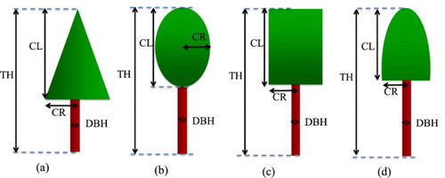
Tree architecture is defined by four parameters: TH, CL, CR, and DBH, as shown in Figure 1. The relationships among the TH, CL, CR, and DBH can be determined from allometric equations, which can be derived through forest inventories. In traditional forestry, the architectural parameters are related to an easily measurable primary variable, usually the DBH. Nevertheless, from the perspective of remote sensing, TH is a more easily available parameter than DBH from spaceborne or airborne observations. Therefore, we made re-calibrated models to estimate CL, CR, and DBH based on TH in this study.

3.2. Statistical distribution models of TH and tree location

The distribution of TH can usually be described by a two-parameter Weibull distribution (Siipilehto 2006), whose probability density function is as follows:(1) where x ≥ 0 is the random variable; k > 0 is the shape parameter; and λ > 0 is the scale parameter of the distribution. The cumulative distribution function for the Weibull distribution is a stretched exponential function as follows:(2) The parameters k and λ were determined by fitting with the real statistical distribution of TH through non-linear optimization. Heights of individual trees are determined by using a group of random numbers to make the distribution of TH values satisfy the above Weibull distribution.

To describe the spatial distribution of tree locations within a domain, we divided the domain into a number of quadrats. The number of trees within a quadrat is often assumed to be randomly distributed in a traditional 3-D RT simulation of forest stands (Wu and Strahler 1994). Accordingly, the possibility of finding x trees in a quadrat can be described using Poisson theory:(3) where m is the average number of trees within each quadrat. The value of m was calculated from the field data set in this study.

However, in some forests, tree locations are not randomly distributed, but rather grouped together in various ways. To model the non-randomness of tree distributions, a Neyman distribution has been used in previous studies (e.g. Franklin et al. 1985; Chen and Leblanc 1997). According to Neyman theory, the probability of having x trees within a quadrat is:(4) where m₁= m²/(ν − m) and m₂= (ν − m)/m; m and ν are the mean and variance of the distribution of tree numbers per quadrat, which were calculated from the field data set in this study. Same as the means to determine TH, the numbers of trees within each quadrat were determined using a group of random numbers to make them satisfy either a Poisson or Neyman distribution (depending on the forest type). The coordinates of individual trees were then randomly located within each quadrat by taking into consideration of reasonable crown overlaps.

3.3. Steps involved in generating simulation of forest stands

According to above-mentioned description, the major steps of the proposed approach for generating forest structures are summarized as follows (also shown in Figure 2):

Figure 2. Framework of the proposed Forest Structure Model (FSM) used to generate a simulated forest stand.

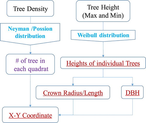
Step 1 is to input the TD within a domain, which will be divided into a number of quadrats. The size of the quadrat depends on the CR.

Step 2 is to determine the number of trees within each quadrat, according to either a Neyman or a Poisson distribution.

Step 3 is to input the maximum and minimum TH (TH_max and TH_min) of the simulated forest stand. Then, the TH for individual trees is determined according to the Weibull distribution.

Step 4 is to calculate the CL, CR, and DBH of individual trees using the predetermined TH and allometric equations derived from the forest inventories.

Step 5 is to determine the spatial positions of individual tress, which are randomly located within each quadrat satisfying a horizontal crown overlap value of 10%.

It should be noted that the forest structure parameters generated by the proposed approach cannot solely drive the running of MCRT models. Several other parameters like LAI, reflectance and transmittance coefficients are also needed, which can be obtained through either field or laboratory measurements.

3.4. Performance assessment

We conducted an RT computation using the FLiES (Kobayashi and Iwabuchi 2008) to evaluate the performance of generated forest structures by simulating the stand BRF for the Järvselja and PFRR sites in this study. FLiES is a 3-D MC ray-racing RT model that has been validated for computing the BRF of forest stands (Kobayashi et al. 2012) and assessed by comparing with other RT models (Widlowski et al. 2013).

Two evaluation experiments were conducted. The first one was to compare the BRF for the measured forest landscapes with the BRF for generated structures from our proposed method. The second one was to compare the simulated BRF using the generated forest structures with the corresponding MODIS reflectance products. The main parameters needed to run the FLiES model are listed in Table 2. The in situ measured LAI values were used in the FLiES simulation, that is, 2.21 and 0.73 for the Järvselja and PFRR sites, respectively. Optical properties consist of a needleleaf type leaf spectral reflectance and transmittance, woody reflectance (medium reflectivity) and floor reflectance (average reflectivity of moss and lichen) data sets. These optical data were compiled from existing literatures and publicly available data sets, provided by Kobayashi (2015). Regarding the observation geometry, the BRF within the principle plane was calculated in the first experiment with the solar zenith angles of 40° and 60°, and the view zenith angles ranging from 0° to 70°, with an interval of 10°; in the second experiment, observation geometry provided by MODIS products were used for each study site.

Table 2. Input parameter to the FLiES model.

Parameter	PFRR site	Järvselja site
LAI	0.73	2.21
Spherical average shoot silhouette to total area ratio^a	0.158	0.158
Needle reflectance	(0.058, 0.428, 0.052, 0.116, 0.387, 0.252, 0.235)^b	(0.058, 0.428, 0.052, 0.116, 0.387, 0.252, 0.235)^b
Needle transmittance	(0.037, 0.390, 0.021, 0.087, 0.372, 0.237, 0.000)^b	(0.037, 0.390, 0.021, 0.087, 0.372, 0.237, 0.000)^b
Stem reflectance	(0.225, 0.461, 0.147, 0.210, 0.606, 0.582, 0.264)^b	(0.225, 0.461, 0.147, 0.210, 0.606, 0.582, 0.264)^b
Floor reflectance	(0.124, 0.280, 0.062, 0.086, 0.376, 0.297, 0.178)^b	(0.124, 0.280, 0.062, 0.086, 0.376, 0.297, 0.178)^b
Forest landscape	Generated by the proposed approach of this study	Generated by the proposed approach of this study

^aFrom Kobayashi et al. (2010).

^bValues for MODIS bands 1–7.

Two indices, root mean square error (RMSE) and relative RMSE (rRMSE), were used to assess the performances of the proposed method. The indices are defined as follows:(5) (6) where X_mea,i and X_gen,i are the BRFs for the measured and simulated forest structures, respectively; and N is the number of the BRF samples. The correlation between the two types of BRFs was also calculated.

4. Results

4.1. Validation of the statistical distributions of TH and tree location

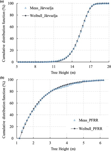
In this study, the Weibull distribution was applied to fit the real statistical distribution of TH for both the Järvselja and PFRR sites. Practically, the fitting was performed based on the cumulative probability through non-linear optimization. To make random variable x in Equation (1) range from zero, it was defined as x = TH − TH_min, where the TH_min is the minimum TH of a forest stand. Figure 3 shows a comparison between the statistical distribution of the measured TH and the fitted cumulative probability using the two-parameter Weibull distributions. It can be seen that the Weibull functions fit the real distributions very well for both sites. The shape and scale parameters (k and λ, respectively, in Equation (2)) were 8.56 and 10.48 for the Järvselja site, and 1.04 and 1.2 for PFRR site, respectively. These results demonstrate that the Weibull distribution is flexible enough to reproduce the statistical distribution of TH within a forest stand. Therefore, the fitted Weibull distributions were used in the generation of the forest structures.

Figure 3. Statistical distributions of TH at the (a) Järvselja and (b) PFRR sites, compared to the Weibull distributions.

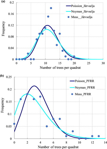
To describe the statistical distribution of tree locations at the two study sites, we divided the measurement plots into 100 quadrats. The quadrat sizes were 10 × 10 m and 3 × 3 m for the Järvselja and PFRR sites, respectively. The quadrat sizes were different because the areas of sampling plots were different for the two sites (100 × 100 m for Järvselja, and 30 × 30 m for PFRR). The frequencies for each value of tree numbers located within one quadrat were calculated. Then the Poisson and Neyman distributions were applied to fit the frequency values, using the parameters determined according to Equations (3) and (4), respectively. As shown in Figure 4(a), the Poisson distribution yielded slightly better agreements with the measured possibilities than the Neyman distribution for the Järvselja site. In contrast, for the PFRR site, the Neyman distribution noticeably outperformed the Poisson distribution in fitting the measured possibility values (Figure 4(b)). It indicates that the distribution of tree locations in the PFRR site was prone to a non-random distribution. Thus, the Poisson and Neyman distributions were utilized separately to generate the modeled forest landscapes for the Järvselja and PFRR sites.

Figure 4. Statistical distributions of tree locations at the (a) Järvselja and (b) PFRR sites, obtained by dividing the measurement plot into 100 quadrats, and then compared to the Poisson and Neyman distributions.

4.2. Comparison between the measured and simulated forest landscapes

Using the parameters determined above, we simulated two forest landscapes with the same TD values for the two study sites, respectively, as shown in Figure 5(a,c). Parallel comparisons of the measured landscapes were shown in Figure 5(b,d). The statistical descriptions of the landscape parameters are summarized in Table 3. For the Järvselja site, the average and standard deviation values of TH, CL, CR, and DBH of the modeled landscape were all slightly lower than those of the measured landscape. The underestimation of CR made the crown coverage of the modeled landscape was about 10% lower than that of the measured landscape. On the other hand, the crown coverage for the modeled PFRR site was close to that of the measured landscape with a difference of 2.9%.

Figure 5. Vertical view of (a) the modeled forest stand, and (b) the measured stand at the Järvselja site; (c) the modeled forest stand and (d) the measured stand at the PFRR site. CC, crown coverage.

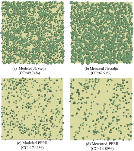
Table 3. Descriptive statistics of the structural parameters of the measured and modeled forest stands at the Järvselja and PFRR sites.

	TH (m)	CL (m)	CR (m)	DBH (cm)	TD (ha^−1)	CC (%)
Järvselja_measured	15.48 (1.51)	4.05 (1.01)	1.44 (0.47)	17.34 (4.44)	1121	62.91
Järvselja_modeled	14.85 (1.45)	3.57 (0.93)	1.22 (0.42)	15.39 (3.93)	1121	49.74
PFRR_measured	2.44 (1.07)	1.96 (1.07)	0.38 (0.04)	2.42 (1.59)	3967	14.89
PFRR_modeled	2.42 (1.33)	1.94 (0.76)	0.38 (0.04)	1.48 (0.76)	3967	17.11

Notes: TH, tree height; CL, crown length; CR, crown radius; DBH, diameter at breast height; TD, tree density; and CC, crown coverage. Values in brackets are standard deviations.

4.3. Comparisons of the computed BRF for generated and measured forest structures

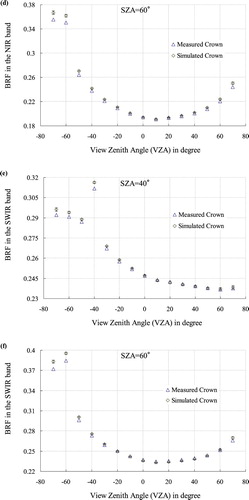
The BRF in the red, NIR, and SWIR bands were calculated using the FLiES model for the Järvselja and PFRR sites. To test the robustness of the proposed approach, 50 forest landscapes were generated for each site by repeating the random numbers for determining the THs and tree locations. Figure 6 shows the averages and standard deviations of the calculated BRF for the 50 generated forest landscapes at the Järvselja site, compared with the BRF for the measured landscape. Standard deviation values lower than 0.003 were derived, indicating that variations caused by using different random numbers were negligible. The average BRF for the modeled landscapes demonstrated high agreement with the BRF for the measured landscape with absolute differences lower than 0.01. Nevertheless, a slight underestimation (absolute error of lower than 0.01) of red BRF was observed (Figure 6(a,b)). This is because the modeled landscape had a lower crown coverage than the measured one. In the red band, photons are much more readily absorbed rather than scattered by the canopies. It should be noted that the absolute error of 0.01 is within the range of theoretical accuracy of atmospheric correction algorithm (with absolute error ranging 0.003∼0.014) for MODS reflectance product (Vermote and Vermeulen, 1999). In contrast, in the NIR and SWIR bands, scattering is much stronger than absorption. Therefore, the lower crown coverage did not yield noticeable discrepancies for the NIR and SWIR bands (Figure 6(c–f)). Table 4 summarizes the values of the evaluation indices for the comparisons. For all the spectral bands, the RMSE values were lower than 0.01. However, the rRMSE values for the red band were around 19%, higher than the values for the NIR and SWIR bands, which were around 3%. The large rRMSE values resulted from the fairly low magnitude of BRF in the red band, compared with the BRF in the NIR and SWIR bands.

Figure 6. Comparisons of computed BRF, based on the measured and simulated forest stands for the Järvselja site. The BRF computation was conducted in the principle plane, using the measured LAI of 2.21. The error bars indicate the standard deviation of the computed BRF corresponding to the 50 simulated stands using different random numbers.

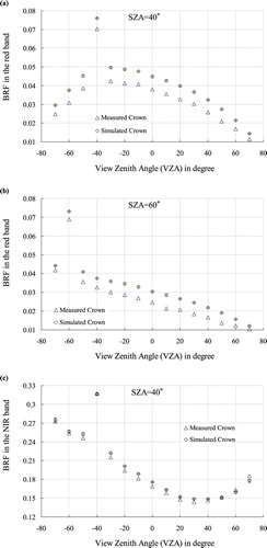
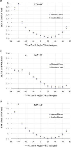
Table 4. Performance assessment of the proposed method for deriving RT simulations of BRF of forest stand.

		Järvselja		PFRR
		SZA = 40°	SZA = 60°	SZA = 40°	SZA = 60°
Red	R^2	0.99	0.99	0.99	0.99
	RMSE	0.006	0.005	0.002	0.002
	rRMSE (%)	19.02	19.82	2.24	2.63
NIR	R^2	0.99	0.99	0.99	0.99
	RMSE	0.005	0.008	0.002	0.005
	rRMSE (%)	2.72	3.32	0.81	2.16
SWIR	R^2	0.99	0.99	0.99	0.99
	RMSE	0.006	0.006	0.002	0.004
	rRMSE (%)	2.69	2.49	0.74	1.6

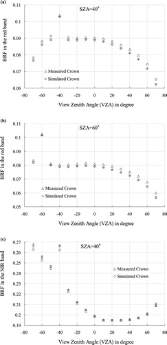
It was not surprising to see a high agreement between the BRF for the modeled and measured landscapes at the PFRR site (Figure 7), because the statistical properties of the landscape parameters were very similar (as summarized in Table 3). Specifically, the difference of the BRF in the red band was lower than 0.003 (Figure 7(a,b)), which was noticeably smaller than at the Järvselja site (Figure 6(a,b)). Quantitatively, the RMSE values for the red, NIR, and SWIR bands were not higher than 0.006, and the rRMSE values were all lower than 3%. All of the results demonstrated a high consistency between the modeled and measured landscapes when simulating the BRF of forest stands with the relative errors for red, NIR, and SWIR bands lower than the theoretic errors for atmospheric correction algorithm of MODIS reflectance product (Vermote and Vermeulen, 1999). Moreover, standard deviation of the computed BRF for the 50 generated forest landscapes were also very low for the PFRR site.

Figure 7. Same as Figure 6 but for the PFRR site. The LAI used in the BRF simulation was 0.73, that is, the measured value at the site.

4.4. Sensitivity analysis

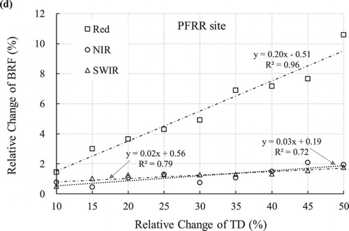
Simulation experiments were conducted to test the sensitivity of BRF variations to TH and TD by changing one factor at a time. That is, in each simulation experiment, only one factor (either TH or TD in this study) was changed, while the other parameters were kept as their baseline values. For example, in the sensitivity experiment of TH, only the TH values of individual trees were changed, but the other parameters, like LAI, TD, and optical properties, were kept as the field measured constants. Specifically, the TD values were changed from 357 to 643 ha⁻¹ and from 564 to 1003 ha⁻¹ for the PFRR and Järvselja sites, respectively; the average TH values were changed from 2.42 to 5.02 m and from 8.97 to 14.31 m for the PFRR and Järvselja sites, respectively. The variation of input and output parameters was quantified by relative change, which is defined as the percentage ratio of absolute change to baseline value.

Figure 8 shows the regression analysis results between the relative changes of BRF in red, NIR, and SWIR bands versus the relative changes of mean TH and TD of the generated forest stands for the Järvselja and PFRR sites. Significant correlations were derived with coefficient of determinations ranging from 0.72 to 0.98, indicating that the changes of TH and TD may cause the variations of BRF simulations. The BRF in red band showed higher sensitivity to changes of TH and TD than the BRF in NIR and SWIR bands, with the regression slopes ranging from 0.20 to 1.16. In contrast, the slopes for NIR and SWIR bands ranged from 0.03 to 0.20 and from 0.02 to 0.17, respectively. This is caused by the noticeably lower magnitudes of BRF in the red band than in the NIR and SWIR bands (see Figures 6–7). The Järvselja site yielded higher sensitivity to changes of TH and TD than the PFRR site. This is because the Järvselja site was much denser than the PFRR site with threetimes higher overstory LAI. For the PFRR site, a relative change of around 50% for TH or TD only caused a relative change of less than 10% for BRF, which was mainly due to the sparse TD with a low overstory LAI of 0.73 and a crown coverage of 17%.

Figure 8. Relative changes of BRF vs. relative changes of TH for (a) the Järvselja site and (c) the PFRR site; and vs. relative changes of TD for (b) the Järvselja site and (d) the PFRR site.

4.5. Comparison with the MODIS reflectance

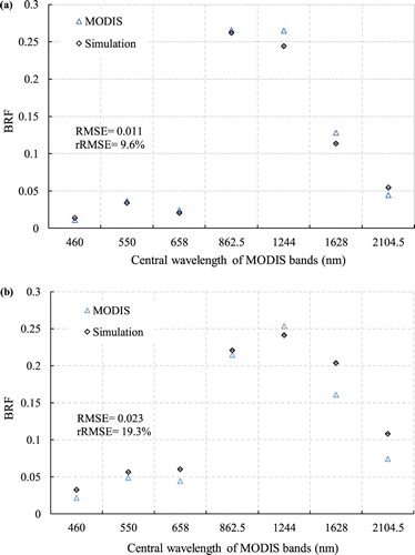
The computed BRF using the generated forest landscapes and in situ measured LAI was then compared with the corresponding MODIS reflectance data for the two study sites. As shown in Figure 9, the computed spectra of BRF showed high agreements with the MODIS spectra. Specifically, RMSE and rRMSE for the Järvselja site were around 0.01 and lower than 10%, respectively, compared with those around 0.02 and lower than 20% for the PFRR site. These results demonstrate the potential of our proposed method for generating forest structures to develop estimation algorithms of ECVs based on satellite observations.

Figure 9. Comparison of MODIS and simulated BRF for (a) the Järvselja site and (b) the PFRR site.

5. Discussion and conclusions

In this study, we developed a statistical approach to generate forest structures of intermediate complexities for driving the 3-D MCRT simulations of BRF. The proposed approach is essentially based on the statistical distribution models of THs and tree locations; and the tree architectures are determined according to allometric equations. It should be noted that the objective of the proposed approach is not to generate the forest structures same as the field measured structures, but aims at facilitating applications of MCRT models to develop remote sensing retrieval algorithms. Therefore, it was validated by comparing the computed stand-level BRF based on the field measured forest structures and the generated structures from our proposed approach for two boreal forest sites. Validation results demonstrated that the computed BRF from a MCRT model utilizing the measured forest stands agreed well with the computed BRF utilizing the generated forest stands from our proposed approach. Comparison of the computed BRF with corresponding MODIS reflectance data also yielded high agreements for the two study forest sites with RMSE and rRMSE lower than 0.03 and 20%, respectively. These results showed that the proposed approach can generate forest stand structures to drive the 3-D MCRT models with simulation accuracies of BRF higher than the theoretical accuracy of atmospheric correction algorithm for MODIS reflectance product (Vermote and Vermeulen, 1999).

Compared to the existing Disney-model (Disney et al. 2006), which can generate very detailed 3-D forest structures, the main merit of our approach is that it can be simply implemented to generate forest structures with intermediate complexities. In the Disney-model, the so-called Treegrow model (Leersnijder 1992) was adopted to generate detailed tree architectures. However, it is a hard task to apply the Treegrow model to variable forest biomes because more than 40 parameters must be empirically tuned for different forest types. In contrast, our proposed approach generates the tree architectures in a simpler way by treating the canopy crowns as abstract geometry objects (see Figure 1). Existing validation results for RT models have indicated that the abstraction scheme of tree architectures is an effective method for simulating stand reflectance and radiation fluxes, with no loss of simulation accuracy (e.g. Kobayashi and Iwabuchi 2008; Kobayashi et al. 2010, 2012). In our proposed approach, the descriptive parameters of canopy crowns are determined according to the allometric equations. Practically, the heights of individual trees are first determined following a Weibull distribution, with the descriptive parameters, including CL, CR, and DBH, then estimated accordingly. Therefore, even if we take a statistical approach to generate forest structure, it has more complexities of explicit information of diverse THs and crown structures than the classical GO-RT models (e.g. Li et al. 1995).

Although our approach has only been validated at two boreal forest stands in this study, the widely published allometric equations for a variety of forest biomes make it possible to be applied to different forest types. For example, Kato et al. (1978), Buba (2013), and Ishihara et al. (2015) presented the allometric equations for tropical forests, Savannas, and temperate forests, respectively.

Besides the above-mentioned allometric equations, the inputs of THs and TDs as well as the distribution parameters are also needed to generate typical stand structures for global forests. Fortunately, the public availability of a global wall-to-wall TH product (spatial resolution of 1 km, Simard et al. 2011) and a global TD product (spatial resolution of 1 km, Crowther et al. 2015) makes the inputs of our proposed approach obtainable at the global scale. Moreover, spaceborne/airborne LiDAR and tree census measurements can provide tree size distributions (e.g. Stark et al. 2015), which helps to parameterize the statistical distributions of TH and tree locations. Thus, our proposed approach is currently the only feasible technique for studying the forest structures at continental to global scales. Nevertheless, more validations in difference biome types are still needed because of the limited validations in this study.

By using more realistic forest structures generated by our approach, it consequently provides an opportunity to develop novel retrieval algorithms of ECVs based on the MCRT models. It may reduce the uncertainties of existing satellite products of ECVs, such as the LAI in sparsely vegetated and savanna areas (Fang et al. 2013). Therefore, generation of typical stand structures for global forest biomes and assessment of their applications to develop retrieval algorithms will be the focus of future studies.

Acknowledgements

The forest census data at Järvselja were provided by Dr Andres Kuusk. The forest census data at Poker Flat Research Range were obtained by a JAMSTEC and IARC-UAF collaboration study. This study was conducted under the JAXA GCOM Research Announcement (the 4th RA102 and the 6th RA 111).

Disclosure statement

No potential conflict of interest was reported by the authors.

References

- Buba, T. 2013. “Relationships Between Stem Diameter at Breast Height (DBH), Tree Height, Crown Length, and Crown Ratio of Vitellaria paradoxa C.F. Gaertn in the Nigerian Guinea Savanna.” African Journal of Biotechnology 12: 3441–3446.
- Chen, J. M., and S. G. Leblanc. 1997. “A Four-scale Bidirectional Reflectance Model Based on Canopy Architecture.” IEEE Transactions on Geoscience and Remote Sensing 35: 1316–1337. doi: 10.1109/36.628798
- Crowther, T. W., H. B. Glick, K. R. Covey, C. Bettigole, D. S. Maynard, S. M. Thomas, J. R. Smith, et al. 2015. “Mapping Tree Density at a Global Scale.” Nature 525: 201–205. doi: 10.1038/nature14967
- Deng, F., J. M. Chen, S. Plummer, S. Mingzhen Chen, and J. Pisek. 2006. “Algorithm for Global Leaf Area Index Retrieval Using Satellite Imagery.” IEEE Transactions on Geoscience and Remote Sensing 44: 2219–2229. doi: 10.1109/TGRS.2006.872100
- Disney, M., P. Lewis, and P. Saich. 2006. “3D Modelling of Forest Canopy Structure for Remote Sensing Simulations in the Optical and Microwave Domains.” Remote Sensing of Environment 100: 114–132. doi: 10.1016/j.rse.2005.10.003
- Fang, H., C. Jiang, W. Li, S. Wei, F. Baret, J. M. Chen, J. Garcia-Haro, et al. 2013. “Characterization and Intercomparison of Global Moderate Resolution Leaf Area Index (LAI) Products: Analysis of Climatologies and Theoretical Uncertainties.” Journal of Geophysical Research 118: 529–548.
- Franklin, J., J. Michaelsen, and A. H. Strahler. 1985. “Spatial Analysis of Density Dependent Pattern in Coniferous Forest Stands.” Vegetatio 64: 29–36. doi: 10.1007/BF00033451
- GCOS. 2011. Systematic Observation Requirements for Satellite-Based Products for Climate, 2011 Update, Supplemental Details to the Satellite-Based Component of the Implementation Plan for the Global Observing System for Climate in Support of the UNFCCC (Reference Number GCOS-154), 138. http://www.wmo.int/pages/prog/gcos/Publications/gcos-154.pdf.
- Ishihara, M. I., H. Utsugi, H. Tanouchi, M., Aiba, M., Kurokawa, H., Onoda, Y., M. Nagano, et al. 2015. “Efficacy of Generic Allometric Equations for Estimating Biomass: A Test in Japanese Natural Forests.” Ecological Applications 25: 1433–1446. doi: 10.1890/14-0175.1
- Kato, R., Y. Tadaki, and F. Ogawa. 1978. “Plant Biomass and Growth Increment Studies in Pasoh Forest.” Malayan Nature Journal 30: 211–224.
- Knyazikhin, Y., J. V. Martonchik, R. B. Myneni, D. J. Diner, and S. W. Running. 1998. “Synergistic Algorithm for Estimating Vegetation Canopy Leaf Area Index and Fraction of Absorbed Photosynthetically Active Radiation from MODIS and MISR Data.” Journal of Geophysical Research: Atmospheres 103: 32257–32275. doi: 10.1029/98JD02462
- Kobayashi, H. 2015. “ Leaf, Woody and Background Optical Data for GCOM-C LAI/FAPAR Retrieval.” JAXA GCOM-C RA4 #102 Project Documents. Available from the author upon the request.
- Kobayashi, H., D. Baldocchi, Y. Ryu, Q. Chen, S. Ma, J. L. Osuna, and S. L. Ustin. 2012. “Modeling Energy and Carbon Fluxes in a Heterogeneous Oak Woodland: A Three-Dimensional Approach.” Agricultural and Forest Meteorology 152: 83–100. doi: 10.1016/j.agrformet.2011.09.008
- Kobayashi, H., H. Delbert, R. Suzuki, and K. Kushida. 2010. “A Satellite-based Method for Monitoring Seasonality in the Overstory Leaf Area Index of Siberian Larch Forest.” Journal of Geophysical Research 115. doi:10.1029/2009JG000939.
- Kobayashi, H., and H. Iwabuchi. 2008. “A Coupled 1-D Atmosphere and 3-D Canopy Radiative Transfer Model for Canopy Reflectance, Light Environment, and Photosynthesis Simulation in a Heterogeneous Landscape.” Remote Sensing of Environment 112: 173–185. doi: 10.1016/j.rse.2007.04.010
- Kobayashi, H., R. Suzuki, S. Nagai, T. Nakai, and Y. Kim. 2014. “Spatial Scale and Landscape Heterogeneity Effects on FAPAR in an Open-Canopy Black Spruce Forest in Interior Alaska.” IEEE Geoscience and Remote Sensing Letters 11: 564–568. doi: 10.1109/LGRS.2013.2278426
- Kuusk, A., M. Lang, J. Kuusk, T. Lukk, T. Nilson, M. Mottus, M. Rautiainen, and A. Eenmae. 2012. “ Database of Optical and Structural Data for the Validation of Radiative Transfer Models.” Tartu Observatory.
- Leblanc, S. G., and J. M. Chen. 2000. “A Windows Graphic User Interface (GUI) for the Five-scale Model for Fast BRDF Simulations.” Remote Sensing Reviews 19: 293–305. doi: 10.1080/02757250009532423
- Leersnijder, R. P. 1992. “ PINOGRAM: A Pine Growth Area Model.” WAU Dissertation 1499. Wageningen Agricultural University, The Netherlands.
- Li, X. W., A. H. Strahler, and C. E. Woodcock. 1995. “A Hybrid Geometric Optical Radiative Transfer Approach for Modeling Albedo and Directional Reflectance of Discontinuous Canopies.” IEEE Transactions on Geoscience and Remote Sensing 33: 466–480. doi: 10.1109/36.377947
- Lovell, J. L., D. L. B. Jupp, D. S. Culvenor, and N. C. Coops. 2003. “Using Airborne and Ground-based Ranging Lidar to Measure Canopy Structure in Australian Forests.” Canadian Journal of Remote Sensing 29: 607–622. doi: 10.5589/m03-026
- Morton, D. C., J. Nagal, C. C. Carabajal, J. Rosette, M. Palace, B. D. Cook, E. F. Vermote, D. J. Harding, and P. R. J. North. 2014. “Amazon Forests Maintain Consistent Canopy Structure and Greenness During the Dry Season.” Nature 506: 221–224. doi: 10.1038/nature13006
- North, P. R. J. 1996. “Three-dimensional Forest Light Interaction Model Using a Monte Carlo Method.” IEEE Transactions on Geoscience and Remote Sensing 34: 946–956. doi: 10.1109/36.508411
- Pinty, B., T. Lavergne, R. E. Dickinson, J. L. Widlowski, N. Gobron, and M. M. Verstraete. 2006. “Simplifying the Interaction of Land Surfaces with Radiation for Relating Remote Sensing Products to Climate Models.” Journal of Geophysical Research 111. doi:10.1029/2005JD005952.
- Pisek, J., and J. M. Chen. 2009. “Mapping Forest Background Reflectivity Over North America with Multi-angle Imaging SpectroRadiometer (MISR) Data.” Remote Sensing of Environment 113: 2412–2423. doi: 10.1016/j.rse.2009.07.003
- Siipilehto, J. 2006. “Height Distributions of Scots Pine Sapling Stands Affected by Retained Tree and Edge Stand Competition.” Silva Fennica 40: 473–486.
- Simard, M., N. Pinto, J. B. Fisher, and A. Baccini. 2011. “Mapping Forest Canopy Height Globally with Spaceborne Lidar.” Journal of Geophysical Research 116. doi:10.1029/2011JG001708.
- Stark, S. C., B. J. Enquist, S. R. Saleska, V. Leitold, J. Schietti, M. Longo, L. F. Alves, P. B. Camargo, R. C. Oliveira, and M. Uriarte. 2015. “Linking Canopy Leaf Area and Light Environments with Tree Size Distributions to Explain Amazon Forest Demography.” Ecology Letters 18: 636–645. doi: 10.1111/ele.12440
- Verhoef, W., and H. Bach. 2003. “Simulation of Hyperspectral and Directional Radiance Images Using Coupled Biophysical and Atmospheric Radiative Transfer Models.” Remote Sensing of Environment 87: 23–41. doi: 10.1016/S0034-4257(03)00143-3
- Vermote, E. F., and A. Vermeulen. 1999. “ Atmospheric Correction Algorithm: Spectral Reflectances (MOD09).” MODIS Algorithm Technical Background Document, NASA.
- Widlowski, J. L., B. Pinty, M. L. Lopatka, C. Atzberger, D. Buzica, M. Chelle, M. Disney, et al. 2013. “The Fourth Radiation Transfer Model Intercomparison (RAMI-IV): Proficiency Testing of Canopy Reflectance Models with ISO-13528.” Journal of Geophysical Research: Atmospheres 118: 6869–6890.
- Widlowski, J. L., M. Taberner, B. Pinty, V. Bruniquel-Pinel, M. Disney, R. Fernandes, J.-P. Gastellu-Etchegorry, et al. 2007. “Third Radiation Transfer Model Intercomparison (RAMI) Exercise: Documenting Progress in Canopy Reflectance Models.” Journal of Geophysical Research 112. doi:10.1029/2006JD007821.
- Wu, Y., and A. H. Strahler. 1994. “Remote Estimation of Crown Size, Stand Density, and Biomass on the Oregon Transect.” Ecological Applications 4: 299–312. doi: 10.2307/1941935
- Yao, T., X. Y. Yang, F. Zhao, Z. S. Wang, Q. L. Zhang, D. Jupp, J. Lovell, et al. 2011. “Measuring Forest Structure and Biomass in New England Forest Stands Using Echidna Ground-Based Lidar.” Remote Sensing of Environment 115: 2965–2974. doi: 10.1016/j.rse.2010.03.019