Assessing the potential for satellite image monitoring of seagrass thermal dynamics: for inter- and shallow sub-tidal seagrasses in the inshore Great Barrier Reef World Heritage Area, Australia

ABSTRACT

Seagrass meadows are at increasing risk of thermal stress and recent work has shown that water temperature around seagrass meadows could be used as an indicator for seagrass condition. Satellite thermal data have not been linked to the thermal properties of seagrass meadows. This work assessed the covariation between 20 in situ average daily temperature logger measurement sites in tropical seagrass meadows and satellite derived daytime SST (sea surface temperature) from the daytime MODIS and Landsat sensors along the Great Barrier Reef coast in Australia. Statistically significant (R² = 0.787–0.939) positive covariations were found between in situ seagrass logger temperatures and MODIS SST temperature and Landsat sensor temperatures at all sites along the reef. The MODIS SST were consistently higher than in situ temperature at the majority of the sites, possibly due to the sensor’s larger pixel size and location offset from field sites. Landsat thermal data were lower than field-measured SST, due to differences in measurement scales and times. When refined significantly and tested over larger areas, this approach could be used to monitor seagrass health over large (10⁶ km²) areas in a similar manner to using satellite SST for predicting thermal stress for corals.

KEYWORDS:

• Seagrass
• temperature
• thermal tolerance
• satellite sea surface temperature
• Landsat
• MODIS
• Great Barrier Reef

1. Introduction

Monitoring and managing seagrasses relies significantly on understanding their spatial and temporal dynamics in relation to environmental conditions. These conditions, including light availability and temperature, have been established as the main factors controlling seagrass health and extent, Figure 1 (Collier, Waycott, and McKenzie 2012; Petus et al. 2014; Campbell, McKenzie, and Kerville 2006; Collier et al. 2016). Seagrasses exhibit latitudinal gradients in spatial distribution in response to sea surface temperature (SST) gradients (McKenzie 2013), and seasonal variability in growth is strongly affected by SST (McKenzie 1994).

Figure 1. (a) Conceptual summary of seagrass attributes (growth, connectivity and species composition) and their relationship to climate change factors. These attributes are affected by ocean acidification and warming through the key indicator photosynthesis: respiration ratio (P:R) (Waycott 2007) and (b) theoretical model of stress response by seagrass populations and communities adapted from Collier, Waycott, and McKenzie (2012).

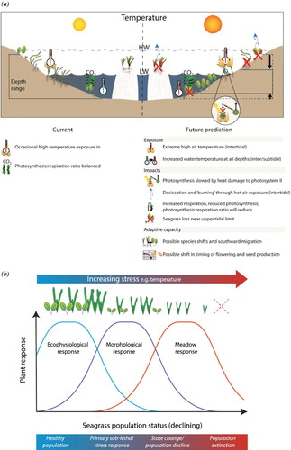
Seagrass meadows are at increasing risk of thermal stress from climate change, particularly those living at their thermal limits (Pedersen et al. 2016) and this will structure futures changes in seagrass distribution (Hendricks, Olsen, and Duarte 2017). Temperature extremes have already contributed to significant seagrass mortality (Thomson et al. 2015; Marba and Duarte 2010). Extensive measurements have shown species-specific thermal optima for seagrass species common in Australia, including Halodule uninervis, Zostera muelleri ssp capricorni, Thalassia hemprichii, and Halophila ovalis (Collier, Uthicke, and Waycott 2011; Pedersen et al. 2016; Adams et al. 2017). Frequent exposure to extreme temperatures above their optima affects seagrass photosystems, reducing and eventually halting photosynthesis, which, combined with increasing respiration rates, results in mortality at seagrass meadow scales (km²), Figure 1, (Collier, Waycott, and McKenzie 2012; Campbell, McKenzie, and Kerville 2006; Collier and Waycott 2014; Pedersen et al. 2016; Olsen et al., forthcoming). As a result, spatial variations in SST produce changes in seagrass plant condition, species diversity and genetic diversity (Reynolds et al. 2016).

At least 34,841 km² of seagrass has been mapped within the boundaries of the Great Barrier Reef World Heritage Area (GBRWHA) (McKenzie et al. 2014, 2010; Coles et al. 2015). The seagrass species in these areas range from smaller growth form grasses and oval leaves of Zostera spp., Syringodium spp. and Halophilla spp. in the south, to more diverse species and growth forms in the north, such as Thalassia spp. (Carruthers et al. 2002; Kirkman 1997; Waycott, Longstaff, and Mellors 2005). Seagrass meadows extend across the GBRWHA mid-shelf reef, lagoon and adjacent coastline, from highly turbid coastal intertidal regions, to shallow coral reefs, and down to 61 m in in lagoonal areas between offshore reefs (Coles et al. 2015; Coles et al. 2009). The Great Barrier Reef (GBR) also includes large areas of seagrass that are difficult and costly to access for routine monitoring. This ecosystem is managed by the GBR Marine Park Authority and the State of Queensland as a significant natural resource underpinning matters of national environmental, cultural and economic significance. Similar extensive seagrass areas, but with different species composition occur on Australia’s western and southern coastlines, throughout Asia, the Pacific Islands, and in North, Central and South America, Europe and Africa (Green and Short 2003). Mapping the presence and condition of seagrasses across the GBR by satellite or airborne remote sensing alone is not possible due to the range of depths and water clarities, and the often sparse cover levels at which seagrasses occur. However, risk to seagrass from known environmental stressors over these large spatial scales could be determined using environmental indicators, such as water temperature.

Seagrass management agencies need effective measures of the spatial and temporal variation in SST, and its extremes, in seagrass meadows. This information, when combined with biologically and location-relevant SST thresholds for seagrass species, can be used to monitor thermal stresses in a manner similar to that used for coral reefs – i.e. degree heating weeks (Heron et al. 2016). We note that seagrasses occur over a wider range of latitudes than corals; hence they will have a greater range of thresholds. There are significant predicted and observed changes in SST associated with global climate change and its more local impacts on the environmental processes that control SST, such as oceanic circulation patterns, tropical cyclones and rainfall patterns (Waycott et al. 2007). While in situ measured temperature has been shown to affect the condition of seagrasses at local scales (1–10² km²), more attention is required to understanding its extremes and their dynamics, and along with recognising substantive latitudinal variation in seagrass forms and thermal tolerances, this needs to be translated to larger areas (10⁶km²) to monitor and assess seagrass response to SST variations. This requires new approaches that build from local scale studies to regional and continental scales. This paper represents a preliminary step towards addressing this problem.

Operational mapping of SST from satellites is a well-developed field with standardised and accurately calibrated and validated global SST data sets produced at least twice daily by satellite imaging systems. These systems have been used extensively to study SST dynamics in and around Australia’s GBRWHA (Heron et al. 2016; Macdonald et al. 2016). Developing an understanding of satellite SST and its relationship to in situ temperatures in seagrass meadows could enable it to be used as an indicator of seagrass condition.

In this paper, we assess the potential for satellite image data to predict water temperature in shallow (above 10 m), and intertidal tropical seagrass meadows throughout the GBRWHA. This would enable us to predict water temperature where logger data are not available. Our first objective was to determine if there was a covariation between in situ average daily temperature logger measurements in seagrass meadows and coincident satellite derived daytime SST from the MODIS (moderate resolution imaging spectrometer) and Landsat enhanced thematic mapper and operational land imager (OLI) thermal sensors. The second objective was to assess the possible impact of tidal variations on in situ temperature and satellite SST measurements to explain systematic differences observed between the two data sets. Addressing both objectives is one of the first preliminary steps that will enable development of satellite SST-based seagrass thermal stress products to potentially assist monitoring and managing seagrass ecosystems. The questions to be addressed relate to the nature of covariation between these data sets and the satellite SST. Given that the MODIS satellite SST is for a 1 km × 1 km window within 3–5 km of the in situ logger locations, and is measuring skin temperature as opposed to air or water column, there should be some differences. Analysing the Landsat sensor’s thermal data and associated water levels over the intertidal areas at image acquisition associated with each logger site should also help to understand some of the dynamics. At a basic level, this will help scientific and management activities focused on seagrass establish the types of variations in thermal properties occurring within intertidal areas where seagrass occurs, although much more detailed work will be required after this initial study.

2. Materials and methodology

Several stages were used to determine if satellite SST could be related to in situ temperature measurements in seagrass meadows along the GBRWHA coast (Figure 3) using freely accessible satellite SST data sets with global coverage. The first two stages assessed the degree of covariation between in situ temperature logger data and satellite SST data derived from the at-surface thermal radiance as measured by the TERRA-MODIS and Landsat 5–8 instruments for the period 2003–2013. Observed differences between field and satellite data were explained by differences in how each of the temperature values was measured. The third stage assessed the impact of tidal variations on in situ temperature and satellite SST to explain systematic differences observed between the two data sets. In the final stage, findings from these initial analyses were used to determine the suitability of satellite SST to provide a regularly updated and spatially extensive tool for monitoring seagrass thermal stress and condition (Figures 2 and 3).

Figure 2. Satellite SST and in situ sensor data processing stream; the dashed boxes indicate objectives 1 and 2.

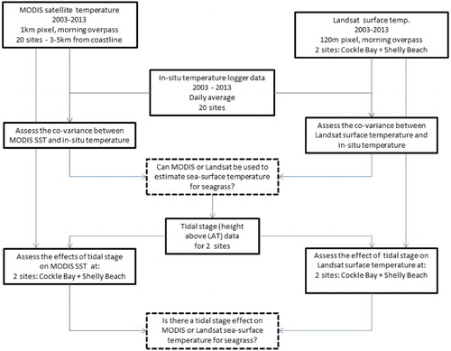
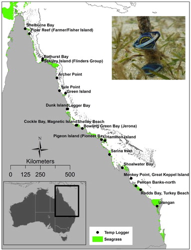
Figure 3. Location of the 20 in situ temperature logging sites in the Great Barrier Reef World Heritage Area (McKenzie et al. 2014). Inset shows an in situ temperature logger (photograph courtesy of Seagrass-Watch).

2.1. Data

2.1.1. In situ seagrass environment temperature measurement

In situ measurements of temperatures in seagrass meadows were collected as part of the GBR Marine Monitoring Program (MMP) at 20 sites from 12° to 24°S along the coast of Queensland for varying periods between September 2003 and July 2013 (McKenzie et al. 2015) (Figure 3). We acknowledge that seagrasses occur over a wider latitudinal range. Autonomous iBTag™ or iBCod™ submersible temperature loggers were deployed at all 20 sites in both shallow subtidal and intertidal meadows. The loggers recorded temperature (accuracy 0.0625°C) within the seagrass canopy every 30–90 minutes (time interval depended on deployment duration and logger storage capacity). Duplicate loggers were attached just above the sediment–water interface to permanent site markers. These ensured sensors were not exposed to air unless the intertidal meadow was completely drained. Average daily temperature was the only parameter available for this analysis and limited our ability to examine hourly and daily variations, especially the occurrence and persistence of extremes at each site. To analyse tidal effects, we conducted more detailed analyses of in situ temperature and satellite SST’s at two sites, Shelley Beach (Townsville, 19° 47′S, 146° 47′E) and Cockle Bay (Magnetic Island, 19° 10′S 146° 49′E). These sites were selected as they are within one Landsat scene and have intertidal seagrass meadows.

2.1.2. Satellite-measured SST

Two of the most common and freely available global archives of satellite-measured surface temperature were accessed: NASA’s MODIS global SST time series and the NASA/USGS series of Landsat satellites’ thermal band. These sensors have different image pixel sizes, 1 km for MODIS (10.78–11.28 µm) and Landsat 5 and 7 (10.40–12.50 µm) and 8 (10.60–11.19 µm) were resampled to 120 m (from 30 m for Landsat 7 and 8) for their thermal bands. The temporal resolution of their collections are also different, with TERRA-MODIS providing a daily daytime collections at 1030hrs local time, while Landsat sensor data were collected every 16 days at approximately 0945hrs local time.

The thermal radiance values derived from atmospheric correction of the satellite image data were converted to brightness temperature using pre-launch calibration coefficients (Wan 1999; USGS 2016; Chander, Markham, and Helder 2009; Markham et al. 2014). Skin temperature is not depth integrated or bulk temperature and only represents the ground or water surface temperature to a depth of several centimetres (Schowengerdt 1997). The MODIS TERRA SST products were derived by M.Canto (Biophysical Ocean Group, University of Queensland) from the NASA OBGP image archive, which had been corrected to surface SST using methods outlined in (Brown and Minnett 1999; NASA 2014; Wan et al. 2002). MODIS SST was extracted for each of the 20 field logger sites using the approach outlined in Section 2.2.1 on a daily basis from 1 January 2003 to 31 December 2013. As not all dates contained a valid SST measurement, this produced sample sizes from n = ∼365–3650. The Landsat TIR data were obtained from two seagrass logger sites (Cockle Bay and Shelley Beach), which fell within one Landsat TM and ETM scene centred on Townsville area. For the time period studied, 2003–2013, 76 cloud-free scenes were located and at-sensor digital number values were converted to at-surface temperature using relevant Landsat 5 and 7 calibration coefficients and ENVI’s FLAASH module with locally derived atmospheric constituent information. These data covered all tidal stages; so in some cases were water surface temperature and in others ground surface temperature.

Match-ups in time to in situ temperature data were provided by: (1) daily cloud-screened MODIS SST data from the 1030 hrs local (0030 GMT) overpass were provided for the period 2003–2013; (2) cloud-screened Landsat 5 (43 images) and 7 (55 images) (2 images) thermal data for 2003–2013 (n = 76 scenes) from the USGS Earth Explorer archive.

2.1.3. Additional data used included

1. tidal height for the two selected intertidal study sites in the Townsville area (Shelley Beach, Townsville) and Cockle Bay, Magnetic Island, adjusted for distance from Townsville Port tidal station (Pers. Comm. Mike Davis, Australian Bureau of Meteorology) and (2) delineation of the intertidal zone (area between mean high and low water marks derived from a full archive Landsat image analysis by Dhanjal-Adams et al. 2016).

2.2. Methodology

2.2.1. Assessing covariance between MODIS and Landsat SST and in situ measurements

Our first stage assessed the degree of covariation between satellite-measured temperatures and the closest in situ field measurement site. This was done to determine if satellite-measured SST could be used to assess the thermal condition of coastal seagrass environments.

Completing this task first required the locations of field measurements to be matched to a suitable image pixel. For MODIS data, this also required that the image pixel contained purely water and was not mixed with areas of land due to the 1 km × 1 km pixel size. To implement this approach, pixels were located at an offset, typically 3–5 pixels or 3–5 km from the coast, either to the north or east of each field measurement location. Landsat thermal data with 120 m pixels were matched directly to in situ field measurement sites.

Average daily temperatures were extracted from field logger data sets at each of the n = 20 sites and 1030hrs temperatures were extracted from the MODIS SST product for the corresponding sites using the approach outlined above. The MODIS image data had missing SST values if the pixel was covered by cloud at the time of acquisition or the viewing geometry was considered too steep. For each of the 20 sites, the field-measured temperatures were matched to corresponding days of MODIS satellite-measured temperature for part or all the period 2003–2013.

In the second stage of the work, a similar approach was completed to match field logger data to suitable cloud-free Landsat 5 and 7 at-surface temperature thermal data using two of the field logger sites in the Townsville area (Shelly Beach and Cockle Bay). This location had two intertidal sites which were able to be located on a map of intertidal extents (Dhanjal-Adams et al. 2016). Landsat image data were acquired at approximately 0945hrs. Due to the smaller pixel size of the Landsat TM, ETM, OLI thermal sensors (resampled to 120 m) compared to MODIS sensor (1 km × 1 km) the field and image data locations could be more closely matched.

2.2.2. Assessing tidal stage effects on satellite SST and seagrass in situ temperature measurements

The final stage of the work used the MODIS and Landsat thermal data sets with field logger data for two of the sites around the city of Townsville (19° 15′S, 146° 49′E) to analyse satellite and field derived temperatures in relation to tidal stage and the amount of water covering each sample site. This was assessed by extracting MODIS SST and Landsat at-surface temperature image data from intertidal areas at two study sites using an intertidal zone map derived from a full archive Landsat image analysis by (Dhanjal-Adams et al. 2016) and analysing these data in relation to tidal stage information at Cockle Bay (Magnetic Island) and Shelly Beach (Townsville). The intertidal zone map shows the area between a selected lowest and highest astronomic tides (Dhanjal-Adams et al. 2016). These locations have a semi-diurnal tides with spring tidal range between 0.9 and 3.8 m low and high water, allowing satellite data collected over a range of tidal stages to be assessed. The 120 m pixels also enabled spatial variations in surface temperature to be assessed at each site. Temperature data were grouped into three classes according to tidal height (height in metres above the lowest astronomical tide) at the time that temperature was recorded: low-tide class (<1.5 m); mid-tide class (1.5–2.5 m) or high-tide class (>2.5 m). Both the Cockle Bay and Shelley Beach sites were considered to be exposed to air at tidal levels <1.5 m as the in situ loggers were exposed to air at 0.7–0.8 m. The ‘low-tide’ category would not necessarily mean that the sites were exposed, but they would have been very shallow, and subject to more temperature variations than the mid- and high-tide classes, which when the temperature were under at least 0.5 m of water.

The approach used has several limitations in relation to the spatial and temporal scales of satellite and field measurements and the actual variable measured: (1) field data are measured at a specific point, either below the water surface or in air (at low tide for some locations) and are a measure of kinetic temperature of the water column or air averaged over a 24 hour period; (2) satellite-measured temperatures are for the time of satellite overpass (1030 or 0945 hrs), collected over a 1 km × 1 km or 120 m × 120 m area and represent the skin temperature of the water surface or intertidal surface, with temperature being brightness temperature and (3) although the field loggers were placed in well-established seagrass meadows covering >100 m², these will vary in size and cover and may not cover an entire Landsat TM, ETM, OLI or MODIS pixel.

3. Results

3.1. Assessing covariation between MODIS SST and in situ measurements – all GBR sites

Assessing each of the 20 in situ seagrass temperature measurement sites against MODIS SST (Figure 4) showed statistically significant positive correlations for all sites in estuarine, coastal, inshore, lagoon islands and reef areas, between field-measured water temperature at seagrass meadows and satellite-measured SST from 1 km × 1 km MODIS data. A latitudinal gradient from north to south is evident from the scatterplots, showing the mean temperature decreasing and range of temperatures increasing as lower minimum temperatures are encountered at southern latitudes. This supports previous findings on the same data set, which showed a significant grouping of seagrass environment temperatures either side of 21°S, with an annual mean temperature of 26.3°C for the northern group and 23.8°C for the southern group (McKenzie et al. 2016).

Figure 4. Daily average field-measured temperature compared to satellite SST from MODIS-TERRA for the closest all ocean pixel at selected sites from north to south along the Great Barrier Reef: (a) Sarina Inlet and (b) Urangan for the period September 2003–July 2013. Due to field logger data gaps and cloud cover in satellite image data the matched data points do not cover every day in this period. Inset maps from Google Earth show the location of field logger sites. The full set of sites is shown in the Appendix.

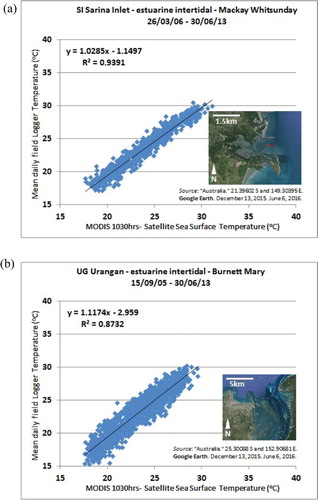
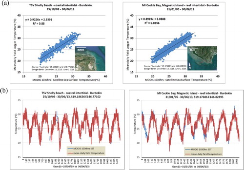
For two selected sites, in addition to the scatterplot of MODIS SST versus in situ temperature (Shelley Beach (Townsville) and Cockle Bay (Magnetic Island) (Figure 5(a)), a time series trace was also produced (Figure 5(b)), which showed the consistency of the positive covariation of the dense in situ logger time series and incomplete MODIS time series across all sites over the 10-year study period. Not all sites covered the full 10-year sample period, with coverage ranging from 12 months to the full 10 years (Appendix). However, a consistent annual pattern was observed with a summer (January–February) maximum and winter (July–August) minimum across all sites in in situ logger temperatures and MODIS SST. Higher frequency temporal variations appear on a scale of 5–7 days, possibly due to local scale (weather, cloud cover and winds) and regional scale (oceanic and tidal currents) effects on water temperature. The slope of the line of best fit between satellite-measured SST and field-measured in situ temperature was typically <1 for all sites, indicating that satellite-measured SST were usually 1–3°C higher than field-measured temperatures. In general, the equations were providing better estimates at 30–32°C, which is the range of temperatures seagrass management agencies and scientists are most interested in. Estimates were more inaccurate at cooler temps (<20°C), or when using them to estimate at higher temperatures (e.g. 40°C). Satellite SST ranged from 1.85°C lower than logged data to 1.76°C more than logged data. There was variability among sites, with coastal–estuarine sites that had larger tidal ranges, and typically more turbid waters, e.g. Pelican Banks, Cockle Bay, Urangan and Shoalwater Bay, experiencing greater variability between in situ an satellite measurements (Blondeau-Patissier et al. 2014). One way of improving the models to adjust for this offset could be to force the equation through the origin point.

Figure 5. Shelley Beach and Cockle Bay, daily average field-measured temperature compared to satellite sea surface temperature from MODIS-TERRA for the closest all ocean pixel, as a scatter plot (a) and time series plot (b) for the period October 2003–June 2013. Due to field logger data gaps and cloud cover in satellite image data the matched data points do not cover every day in this period. Inset map from Google Earth shows the location of the field logger site.

In addition to habitat variability, the differences from field to satellite data may be explained by a number of factors: (1) point based field logger measurement versus a 1 km × 1 km satellite measurement; (2) field measurement in water or air if exposed at low tide and satellite measurement of water surface or exposed intertidal areas at low tide, along with variation in their slope and aspect and (3) locational shift of satellite temperature measurements to sites that were at least 3 km from shore and away from the field sites for the MODIS data to ensure that the pixels sampled consisted of water alone and were not a mixture of water and land (non-intertidal) This last point assumed that the water thermal properties measured would be similar and co-vary with the water thermal properties over the logger site.

3.2. Assessing covariation between Landsat SST and in situ measurements – Townsville area case study

The Landsat 5, 7 and 8 sensor at-surface brightness temperatures extracted for the Cockle Bay and Shelly Beach sites and corresponding field logger site’s in situ temperatures exhibited statistically significant positive covariation over the period of data match-ups obtained from 2003 to 2013 (Figure 6). The Landsat 5, 7 and 8 thermal data exhibited a positive bias in comparison to the in situ logger data over the majority of this period, i.e. consistently recording 1–5°C below the in situ measurements, resulting in a greater range of variation in the fit between satellite and field data. These variations are due to a number of factors addressed in more detail in the Discussion section, including: (1) differences in the measured quantity, (2) differences in area and time between in situ and satellite data, (3) variable water depth and exposure effects and (4) local conditions at the time of image acquisition. It is expected similar variations would be observed at other intertidal sites due to differences in the thermal capacity of substrate and oceanic/tidal waters.

Figure 6. (a) Scatterplots of Landsat 5, 7 and 8 thermal image at-surface brightness temperatures for the Shelley Beach (TSV) and Cockle Bay (MI) study areas (n = 78 and 68, respectively) for 2003–2013 plotted against in situ temperature logger data for the same date, time and location and (b) as a time series plot.

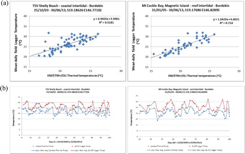
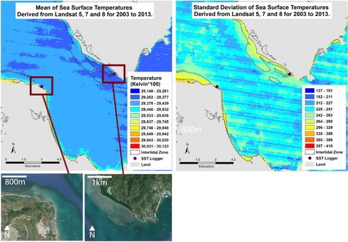
The Cockle Bay and Shelley Beach sites were selected for further investigation as they are intertidal seagrass meadows and exposed for several hours either side of low spring tides, as shown in Figure 7. The Shelley Beach site has low (<20%) seagrass cover, while the Cockle Bay site has areas of 50–100% cover (McKenzie et al. 2016). Examination of the Landsat thermal data within the intertidal polygon showed limited spatial variation (Figure 7 – mean and standard deviation images) in temperature (1–5°C), with greater variation occurring over time at different times of year (Figure 6). Although the Landsat thermal temperatures were lower than the in situ loggers, both showed a similar range in temperatures (10–12°C), 14–26°C for Landsat and 20–32°C for field loggers, over the entire intertidal area and time period sampled. Seasonal variations in SST associated with forcing meteorological and oceanographic conditions may be one factor driving these variations, while tidal stage and degree of exposure are another. The latter is examined in the following section.

Figure 7. Mean and standard deviation of Landsat 5, 7 and 8 thermal images (at-surface brightness temperature) calculated on a per-pixel basis for the Shelley Beach (Townsville; n = 78) and Cockle Bay (Magnetic Island; n = 68) study areas from 2003 to 2013. The areas highlighted within the black polygons are intertidal, as determined from Dhanjal-Adams et al. (2016).

3.3. Assessing tidal stage effects on satellite SST and seagrass in situ temperature measurements

Both in situ logger and Landsat thermal data for the two intertidal sites showed similar trends (Figure 8), with low-tide temperatures appearing higher than temperatures measured at other times. The in situ logger data have temporally consistent differences in temperature, with higher low-tide values, which ranged from 4°C to 8°C higher than high-tide temperatures recorded within the same month (Figure 8(a)). The Landsat thermal data exhibited less consistent differences, in temperature, with higher low-tide values, that ranged from 4°C to 12°C higher than high-tide temperatures recorded within the same month (Figure 8(b)). The observed differences may be due to differences other than tidal stage, as will be discussed in the following section. Statistically significant differences were observed between each different tidal height for MODIS SST measurements in both locations (Figure 9(a)), as determined by unpaired T-tests (p < .05), but not for Landsat temperatures and tidal height (p > .05) (Figure 9(b), Figure 10). The observed differences between low and high-tide conditions may partly be due to low-tide periods resulting in greater areas of substrate and benthos exposed during daylight hours, each of which has a lower thermal capacity than sea-water; so it may heat more quickly than areas covered at mid and high tides. Separating out this effect is covered in the discussion.

Figure 8. (a,b) in situ logger temperatures for the Townsville (Shelley Beach; n = 70) and Magnetic Island (Cockle Bay; n = 49) study areas for 2003–2013 plotted with tidal stage for the same date, time and location. (c,d) Landsat 5, 7 and 8 thermal image at-surface brightness temperatures for the Townsville (Shelley Beach; n = 78) and Magnetic Island (Cockle Bay; n = 68) study areas for 2003–2013 plotted with tidal stage for the same date, time and location. (e,f) MODIS SST for the Townsville (Shelley Beach; n = 808) and Magnetic Island (Cockle Bay; n = 2013) study areas for 2003–2013 plotted with tidal stage for the same date, time and location.

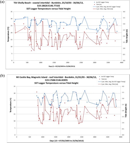
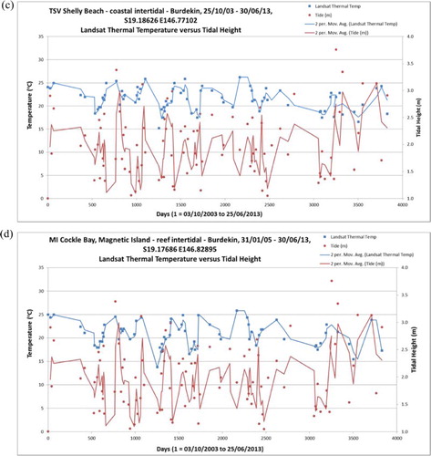
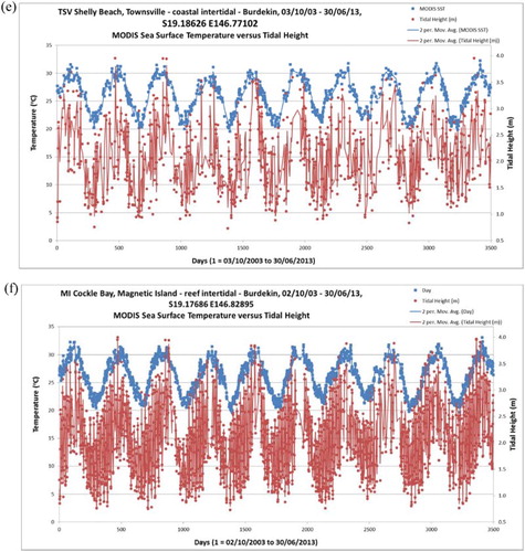
Figure 9. (a,b) Landsat 5, 7 and 8 thermal image at-surface brightness temperature and MODIS SST, for Townsville and Magnetic Island study area aggregated by tidal stage (error bars indicate standard deviation). The number of sites used to assess each tidal stage was low <1.5 m n = 26; mid 1.5–2.5 m n = 38 and high >2.5 m n = 17.

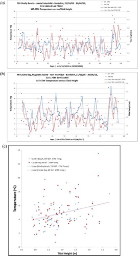
Figure 10. (a,b) Landsat 5, 7 and 8 thermal image at-surface brightness temperature difference with in situ temperature loggers for Townsville and Magnetic Island study area versus tidal stage, and (c) scatterplot of the difference between in situ logger data and Landsat thermal image at-surface brightness temperature versus tidal stage.

4. Discussion

4.1. Assessing covariance between MODIS sensor SST and Landsat surface temperature data with in situ seagrass temperature measurements

The magnitude and timing of temporal variations in both MODIS SST and Landsat surface temperature matched the temporal variations recorded by in situ loggers along the GBR lagoon and coastal sites sampled by this work. The matches were more stable at temperatures of 30–32°C and at sites that were not coastal/estuarine and dominated by turbid waters. The timing of variations able to be detected in these time series extended from daily, weekly, monthly, seasonally and over years in the MODIS SST data due to its daily collection period. Landsat’s 16-day revisit period limited the temporal trends evident in its time series to monthly, seasonally and annually. Both data sets were subject to data gaps due to poor-data collection or cloud cover in the Austral wet-season months of November–April. The loss of data was only significant during extended periods of cloudiness, which were also associated with tropical cyclone occurrences. The dense MODIS time series enabled several trends to be identified. However, quantitative analysis to determine the magnitude and periodicity of temperature variations and power-spectrum analysis was beyond the scope of this work, and represents the next step in building a more detailed understanding of the time scales of variations in SST and the processes driving variations in temperature of the seagrass environment.

The most notable trends in seagrass temperature variations observed from the in situ logger and MODIS SST data that match with known forcing meteorological, oceanographic and climatic conditions were:

• – A relatively stable mean temperature and summer –winter seasonal variation over the sampled period at all sites (Figure 4, Supplementary material – Logger versus MODIS time series);

• – Possible impacts from significant disturbance events, such as tropical cyclones (Larry 2006 and Yasi 2011) and floods from coastal river systems, which appear to reduce temperatures in areas affected by the cyclone path and river flood plume (Supplementary material – Logger versus MODIS time series);

• – Well defined and consistent Austral summer (November–April) temperature maxima to winter (June–September) minima, with a range of 15–17°C and 12–15°C to the south and north of 23°S respectively (Collier et al. 2014). (Supplementary material – Logger versus MODIS time series);

• – Weekly to monthly variations in water temperature may be due to variation in the strength, direction and path of the East Australian Current as it moves southwards along the GBR and interacts with lagoonal and coastal waters, although this effect was not visible in the data and

• – Shorter term, weekly to daily fluctuations, due to local scale (1–100 km²) controls on surface energy exchange, and resultant ground and water surface temperatures; these include meteorological (local wind, irradiance and cloud), water residence time over seagrass meadows due to tidal interactions with local winds and river/creek outflows, and local and non-local swell events. These effects control the area and duration of intertidal areas being exposed and underwater, and are covered in more detail in the next section.

Although there was statistically significant positive covariation measured across all sites between the in situ and satellite measurements, it is important to assess if the data sets being compared are measuring the same physical quantities. There are several differences with respect to what, where, when and how, the in situ and satellite measurements of temperature were made. These need to be established as our underlying assumption is that the physical quantity, measurement techniques, time and location are comparable and can be matched for comparison (Wan 1999; Emery et al. 2001). Figures 4–8 show that this match-up is possible and realistic. The factors required to ensure match-ups are valid, and their known variations are outlined below:

• – Measurement of the same temperature parameter: The in situ loggers are direct contact thermal sensors (iButton© digital thermochron reinforced with solid titanium plates and moulded in a polyurethane casing) and measure kinetic temperature via contact with the water or air they sit in. The MODIS and Landsat TM and ETM thermal sensors measure emitted thermal radiance from set areas on the oceans’ surface or skin (top centimetres) in the 10–11 µm portion of the spectrum. The emitted thermal radiance values are converted to a measurement of surface brightness temperature using a standard calibration equation (Wan 1999; USGS 2016). The difference between measured kinetic versus brightness temperature is that kinetic temperature is the correct internal temperature of a body, while brightness temperature is the apparent temperature, or that measured form longer wavelength energy emitted from the object.

• – Measured area and locations need to match: The in situ loggers record the temperature of the immediate surrounding water or air, effectively within metres and their positions were measured using a standard hand-held GPS unit with positional accuracy of ±3 m (McKenzie et al. 2015). Satellite data were measured within the effective ground resolution element of each sensor, which for MODIS thermal data is 1 km × 1 km and Landsat TM/ETM is 120 m × 120 m. Both data set products used report positional accuracies of approximately 0.5 pixel (Wan 1999). For the MODIS data the sampled pixel was offset from the field logger site to ensure a whole water covered pixel was selected. The Landsat data pixel locations were selected to overlay the field logger sites.

• – Measurement times need to match: The in situ loggers collected data on an hourly basis and for the purposes of this work, the data were aggregated to average daily values (McKenzie et al. 2016). Satellite SST and thermal data were not composited temporally in any way and were obtained at 1030hrs and 0945hrs local time for the MODIS and Landsat data, respectively. The daily range of in situ logger temperature values reached maxima between 1200 and 1400hrs and minima between 0400 and 0600hrs, with values ranging from 15°C to 35°C. The averaging of these data over each 24-hour period would have reduced covariation with satellite-measured SST and surface temperature.

The challenges outlined above are common for validating satellite SST, which is done more typically in the open ocean. However, we have noted the magnitude of these and regard our data sets as comparable, which is supported by similar work (Heron et al. 2016).

4.2. Assessing tidal stage effects on satellite SST and seagrass in situ temperature measurements

Assessing possible tidal stage effects on measured temperatures was challenging. It required separating out variations in measured temperature from day to day cycles in in situ logger temperatures and MODIS SST, and assessing this at a reduced scale for Landsat thermal data. The daily averaged in situ logger data would have reduced the tidal variation effects within the semi-diurnal tidal cycle with any effects being averaged out. MODIS and Landsat measurements will always be at a set point in the tidal cycle due to their consistent morning overpass times. Although the time series plots of Landsat thermal and MODIS SST with tidal stage show almost positive covariation, with low tides often being associated with low temperatures (Figures 8(a,–c), the only statistically significant difference observed was for MODIS SST data between low and high tidal stages. As both MODIS and Landsat over-passes and image-acquisitions are mid-morning, exposed intertidal areas may only have had three to four hours of direct exposure. In warmer months, this may result in heating of the areas measured by temperature loggers and Landsat image pixel values. However, in cooler months, lower temperatures and wind may cool the exposed surfaces and there are greater tidal ranges during the day. Both effects are assumed to occur due to the lower thermal capacity of the substrate in comparison to the water body, i.e. it heats and cools more rapidly than water. Our results show that there may be some form of tidal signal; however, separating this from local scale (1–100 km²) meteorological and oceanographic effects was not possible with the data used in this work. The higher spatial resolution Landsat thermal image data offered some insight into the spatial and temporal dynamics of intertidal seagrass meadows; however, analysis of more frequently collected thermal data would be ideal. This type of assessment requires examination of hourly logger data over intertidal and non-intertidal sites and ideally high spatial resolution thermal images acquired at the same time to examine spatial variation.

4.3. Inferring and monitoring seagrass condition from satellite thermal measurements

One of our initial aims was to address the question of whether we can infer seagrass habitat thermal properties, as typically measured by in situ thermal loggers, from MODIS and Landsat TM/ETM/OLI globally accessible satellite data sets. Our preliminary analyses have shown that, there are indeed statistically significant positive covariations between in situ and satellite-measured temperatures of tropical seagrass meadows of the GBRWHA. However, these relationships within tropical seagrass meadows require further assessment to understand hourly variations in in situ temperature at sites and the extent and persistence of extreme temperatures in in situ and satellite SST. Their usefulness to assess seagrass conditions will need to take into account species and latitudinal variations in seagrass thermal tolerance (Collier et al. 2016; Collier and Waycott 2014; Collier, Waycott, and McKenzie 2012). There are a number of factors likely to cause differences between in situ and satellite measurements, due to measurement extents, approaches and environmental conditions; however, this relationship does appear stable over time and space for the conditions we assessed. Therefore, satellite thermal measurements provide a method for assessing the thermal exposure history of seagrass meadows over weeks to months.

In addition to the more detailed assessments of extremes and seagrass thermal tolerance variability, the following are a number of solutions to address the primary limitations of using satellite-based temperature measurements for assessing seagrass condition and to establish a better understanding of the spatial and temporal scale of their variations. Addressing these limitations will provide a basis for further investigations to directly measure and monitor the thermal environments affecting seagrass over local to regional scales and establish more effective monitoring and management programmes.

• – Develop more precise locational matching between field sample sites and coincident satellite temperature pixels, reducing the offset of satellite pixels away from land to avoid mixed land-water pixels.

• – Develop more effective means to link across in situ and satellite measurement scales, across differences in the spatial scale of sampling units, with field sample sites at points representing temperature within a 1-m² area, and matched satellite temperature pixels collected over 1-km² area.

• – Match the source of temperature measurement, with satellite image data representing sea (subtidal) or substrate (exposed intertidal) surfaces, while field measurements represent seagrass canopy water temperature (subtidal) or air temperature (exposed intertidal).

• – Match the satellite and field logger data temporally, so they both are from the same 30–60 minutes and not daily averages.

• – Develop thermal stress indicators from existing biological response thresholds that can be pragmatically applied to thermal data from remote sensing, i.e. chronic temperature stress, such as degree heating days used for coral reefs.

A major requirement is to develop an understanding of the hourly to daily temporal scale and spatial variations and extremes, in seagrass environment temperatures in the shallow and sometimes exposed intertidal meadows. This is essential to place satellite-measured SST in a context where it can be linked to the in situ scale. Addressing this will require several intensively monitored sites with hourly data from in situ loggers and very high spatial resolution thermal images derived from a fixed thermal camera system. Similar set-ups with relatively low cost approaches have been used at terrestrial sites to understand the thermal and physiological responses of different vegetation communities (e.g. www.supersites.net.au).

Once stable in situ to satellite thermal data relationships are established consideration should also be given to the most suitable form of satellite image data. While Landsat is an operational programme, with an archive extending back to 1972 and forward planning and funding through to 2025, MODIS is a research grade instrument on a NASA research satellite and is well beyond its design life. Ideally, a thermal imaging system with daily overpass, similar to MODIS but with an improved pixel size would be highly suitable. Prediction and forecasting of coral bleaching is operational, and as this is driven by thermal stress, it could be replicated for seagrasses, with a latitudinal varying seagrass thermal exposure satellite image product being calculated from satellite daily SST products (Heron et al. 2016).

Thermal exposure history when combined with thermal stress indicators can be used to identify meadows at risk of thermal stress in a manner similar to degree heating weeks for corals. Temperature thresholds and thermal optima have been identified for a number of the species occurring in the GBR (Pedersen et al. 2016; Adams et al. 2017) and these can be used to develop thermal stress indicators from acute rises in water temperature during heat waves and from water pooling at low tide. Thermal exposure history can also be used to predict and explain changes in species distribution (Collier, Uthicke, and Waycott 2011).

5. Conclusions

Our aim was to determine whether there was significant covariation between in situ average daily temperature logger measurements in tropical seagrass meadows and satellite derived daytime SST from the MODIS and Landsat ETM and OLI thermal sensors. There was statistically significant positive co-variation between the satellite-measured temperatures and the in situ field loggers for all 20 sites examined across the full latitudinal gradient of the GBR (Figure 11). The in situ logger data and daily MODIS SST detected weekly, monthly, seasonal and annual variations in SST. Despite significant differences in the spatial scales and temporal aggregation of the in situ and satellite measurements of temperature, the covariations evident indicate that satellite data can be used to measure and map in situ (with 100 m’s) conditions of seagrass meadows over areas of 10⁶km² on a daily basis. There were significant variations in temperature measurements at different tidal stages evident across field logger and satellite data sets. Only the daily MODIS SST exhibited a statistically significant difference in temperature at intertidal seagrass sites measured between low- and high-tide stages. Lower tidal stages exhibited higher temperatures on average in comparison to mid- and high-tide stages for both Landsat thermal SST and MODIS SST. Significant further work is required with hourly in situ logger data, and possibly drone-based thermal imaging systems, in association with satellite-measured SST, to develop a better understanding of daily seagrass meadow thermal dynamics and extremes in intertidal areas. Investigating the effects of exposure duration and frequency at intertidal sites should also be considered to improve our ability to use temperature data to assess seagrass condition. The knowledge outlined above, along with an assured access to suitable satellite SST time series with pixel sizes of 100 m–1 km, and seagrass species’ thermal tolerance limits, would enable the development of a highly effective seagrass condition assessment tool, as water temperature is a critical factor for seagrass condition and growth.

Figure 11. MODIS SST data mean and standard deviation for their data recording periods for each of the in situ temperature logger locations mapped in Figure 1, progressing from north to south.

Acknowledgements

We thank Dr Scarla Weeks and Marites Canto for the MODIS SST time series and N. Murray, R. Yoshida, N. Smith and L. Langlois for other contributions.

Disclosure statement

No potential conflict of interest was reported by the author(s).

ORCID

S. R. Phinn http://orcid.org/0000-0002-2605-6104

Additional information

Funding

This project is funded by the Great Barrier Reef Foundation’s Resilient Coral Reefs successfully adapting to climate change research and development programme in collaboration with the Australian Government.

References

- Adams, M. P., C. Collier, S. Uthicke, Y. X. Ow, L. Langlois, and K. R. O’Brien. 2017. “Model Fit versus Biological Relevance: Evaluating Photosynthesis-temperature Models for Three Tropical Seagrass Species.” Scientific Reports 7: 39930. doi: 10.1038/srep39930
- Blondeau-Patissier, D., T. Schroeder, V. E. Brando, S. Maier, A. G. Dekker, and S. R. Phinn. 2014. “ESA-MERIS 10-Year Mission Reveals Contrasting Phytoplankton Bloom Dynamics in Two Tropical Regions of Northern Australia.” Remote Sensing 6 (4): 2963–2988. doi:10.3390/rs6042963.
- Brown, O. B., and P. J. Minnett. 1999. “MODIS Infrared Sea Surface Temperature Algorithm – Algorithm Theoretical Basis Document.” University of Miami.
- Campbell, Stuart J., Len J. McKenzie, and Simon P. Kerville. 2006. “Photosynthetic Responses of Seven Tropical Seagrasses to Elevated Seawater Temperature.” Journal of Experimental Marine Biology and Ecology 330: 455–468. doi: 10.1016/j.jembe.2005.09.017
- Carruthers, T. J. B., W. C. Dennison, B. J. Longstaff, M. Waycott, E. G. Abal, L. J. McKenzie, and W. J. Long. 2002. “Seagrass Habitats of Northeast Australia: Models of Key Processes and Controls.” Bulletin of Marine Science 71 (3): 1153–1169.
- Chander, G., B. Markham, and D. Helder. 2009. “Summary of Current Radiometric Calibration Coefficients for Landsat MSS, TM, ETM+ and EO-1 ALI Sensors.” Remote Sensing of Environment 113: 893–903. doi: 10.1016/j.rse.2009.01.007
- Coles, Robert, Len J. McKenzie, Glenn De’ath, Anthony Roelofs, and Warren J. Lee Long. 2009. “Spatial Distribution of Deepwater Seagrass in the Inter-reef Lagoon of the Great Barrier Reef World Heritage Area.” Marine Ecology Progress Series 392: 57–68. doi:10.3354/meps08197.
- Coles, Robert G., Michael A. Rasheed, Len J. McKenzie, Alana Grech, Paul H. York, Marcus Sheaves, Skye McKenna, and Catherine Bryant. 2015. “The Great Barrier Reef World Heritage Area Seagrasses: Managing this Iconic Australian Ecosystem Resource for the Future.” Estuarine, Coastal and Shelf Science 153: A1–A12. doi:10.1016/j.ecss.2014.07.020.
- Collier, C. J., M. P. Adams, L. Langlois, M. Waycott, K. R. O’Brien, P. S. Maxwell, and L. McKenzie. 2016. “Thresholds for Morphological Response to Light Reduction for Four Tropical Seagrass Species.” Ecological Indicators 67: 358–366. doi: 10.1016/j.ecolind.2016.02.050
- Collier, Catherine, Matthew Adams, Paul Maxwell, Len McKenzie, Kate O’Brien, Stuart Phinn, Chris Roelfsema, Sven Uthicke, Kor-Jent van Dijk, and Michelle Waycott. 2014. Seagrass Connectivity, Community Composition and Growth: Attributes of a Resilient GBR. Annual Report 2014 to the Great Barrier Reef Foundation. Brisbane: Great Barrier Reef Foundation.
- Collier, Catherine J., Sven Uthicke, and Michelle Waycott. 2011. “Thermal Tolerance of Two Seagrass Species at Contrasting Light Levels: Implications for Future Distribution in the Great Barrier Reef.” Limnology and Oceanography 56 (6): 2200–2210. doi:10.4319/lo.2011.56.6.2200.
- Collier, C. J., and M. Waycott. 2014. “Temperature Extremes Reduce Seagrass Growth and Induce Mortality.” Marine Pollution Bulletin 83 (2): 483–490. doi:10.1016/j.marpolbul.2014.03.050.
- Collier, C. J., M. Waycott, and L. J. McKenzie. 2012. “Light Thresholds Derived from Seagrass Loss in the Coastal Zone of the Northern Great Barrier Reef, Australia.” Ecological Indicators 23: 211–219. doi: 10.1016/j.ecolind.2012.04.005
- Dhanjal-Adams, K. L., J. O. Hanson, N. J. Murray, S. R. Phinn, V. R. Wingate, K. Mustin, J. R. Lee, J. R. Allan, J. L. Cappadonna, and C. E. Studds. 2016. “The Distribution and Protection of Intertidal Habitats in Australia.” Emu 116 (2): 208–214. doi: 10.1071/MU15046
- Emery, W. J., Sandra Castro, G. A. Wick, Peter Schluessel, and Craig Donlon. 2001. “Estimating Sea Surface Temperature from Infrared Satellite and In situ Temperature Data.” Bulletin of the American Meteorological Society 82 (12): 2773. doi:10.1175/1520-0477(2001)082<2773:ESSTFI>2.3.CO;2.
- Green, E. P., and F. T. Short. 2003. World Atlas of Seagrasses, 298. Berkeley: University of California Press.
- Hendricks, I. E., Y. S. Olsen, and C. M. Duarte. 2017. “Light Availability and Temperature, Not Increased CO2, Will Structure Future Meadows of Posidonia Oceania.” Aquatic Botany 139: 32–36. doi: 10.1016/j.aquabot.2017.02.004
- Heron, Scott F., Lyza Johnston, Gang Liu, Erick F. Geiger, Jeffrey A. Maynard, Jacqueline L. De La Cour, Steven Johnson, Ryan Okano, David Benavente, and Timothy F. R. Burgess. 2016. “Validation of Reef-scale Thermal Stress Satellite Products for Coral Bleaching Monitoring.” Remote Sensing 8 (1): 59. doi: 10.3390/rs8010059
- Kirkman, H. 1997. Seagrasses of Australia. State of the Environment Technical Paper Series (Estuaries and the Sea), 36. Canberra: Department of the Environment.
- Macdonald, H. S., M. Roughan, M. E. Baird, and J. Wilkin. 2016. “The Formation of a Cold-core Eddy in the East Australian Current.” Continental Shelf Research 15: 72–84. doi: 10.1016/j.csr.2016.01.002
- Marba, Nuria, and Carlos M. Duarte. 2010. “Mediterranean Warming Triggers Seagrass (Posidonia Oceanica) Shoot Mortality.” Global Change Biology 16 (8): 2366–2375. doi: 10.1111/j.1365-2486.2009.02130.x
- Markham, B., J. Barsi, G. Kvaran, L. Ong, E. Kaita, S. Biggar, J. Czapla-Myers, N. Mishra, and D. Helder. 2014. “Landsat-8 Operational Land Imager Radiometric Calibration and Stability.” Remote Sensing 6 (12): 12275–12308. doi: 10.3390/rs61212275
- McKenzie, L. J. 1994. “Seasonal Changes in Biomass and Shoot Characteristics of a Zostera Capricorni Aschers. Dominant Meadow in Cairns Harbour, Northern Queensland.” Australian Journal of Marine and Freshwater Research, no. 45: 1337–1352. doi:10.1071/MF9941337.
- McKenzie, Len J. 2013. “Long-term In situ Temperature Monitoring within Inshore GBR Seagrass Meadows.” In Community Compositional Changes and Temperature Thresholds Workshop, Conducted for the Great Barrier Reef Foundation Project ‘Seagrass Connectivity, Community Composition and Growth: Attributes of a Resilient GBR’. St Lucia: Global Change Institute, University of Queensland. 8th October. http://bit.ly/2aVzBjc.
- McKenzie, L. J., C. J. Collier, L. A. Langlois, R. L. Yoshida, N. Smith, M. Takahashi, and M. Waycott. 2016. Marine Monitoring Program: Inshore Seagrass, Annual Report for the Sampling Period 1st June 2014–31st May 2015. Townsville: Great Barrier Reef Marine Park Authority.
- McKenzie, Len J., Catherine Collier, Lucas Langlois, Rudi Yoshida, Naomi Smith, and Michelle Waycott. 2015. Reef Rescue Marine Monitoring Program – Inshore Seagrass, Annual Report for the Sampling Period 1st June 2013–31st May 2014. Cairns: TropWATER, James Cook University.
- McKenzie, Len J., Rudolf L. Yoshida, Alana Grech, and Robert Coles. 2010. Queensland Seagrasses. Status 2010 – Torres Strait and East Coast. Cairns: Fisheries Queensland (DEEDI).
- McKenzie, Len J., Rudolf L. Yoshida, Alana Grech, and Robert Coles. 2014. “Composite of Coastal Seagrass Meadows in Queensland, Australia – November 1984 to June 2010.” PANGAEA. doi:10.1594/PANGAEA.826368.
- NASA 2014. “MODIS-Terra Ocean Color Data.” NASA Goddard Space Flight Center, Ocean Ecology Laboratory, Ocean Biology Processing Group.
- Olsen, Y. S., C. J. Collier, Y. X. Ow, and G. A. Kendrick. Forthcoming. “Global Warming and Ocean Acidification: Effects on Australian Seagrass Ecosystems.” In Seagrasses of Australia, edited by A. W. D. Larkum, G. A Kendrick and P. J. Ralph.
- Pedersen, O., T. D. Colmer, J. Borum, A. Zavala-Perez, and G. A. Kendrick. 2016. “Heat Stress of Two Tropical Seagrass Species During Low Tides – Impact on Underwater Net Photosynthesis, Dark Respiration and Diel In situ Internal Aeration.” New Phytologist 210 (4): 1207–1218. doi:10.1111/nph.13900.
- Petus, Caroline, Catherine Collier, Michelle Devlin, Michael Rasheed, and Skye McKenna. 2014. “Using MODIS Data for Understanding Changes in Seagrass Meadow Health: A Case Study in the Great Barrier Reef (Australia).” Marine Environmental Research 98: 68–85. doi: 10.1016/j.marenvres.2014.03.006
- Reynolds, Laura K., Katherine DuBois, Jessica M. Abbott, Susan L. Williams, and John J. Stachowicz. 2016. “Response of a Habitat-forming Marine Plant to a Simulated Warming Event Is Delayed, Genotype Specific, and Varies with Phenology.” PloS One 11 (6): e0154532. doi:10.1371/journal.pone.0154532.
- Schowengerdt, R. A. 1997. Remote Sensing. Models and Methods for Image Processing. 2nd ed. New York: Academic Press.
- Thomson, Jordan A., Derek A. Burkholder, Michael R. Heithaus, James W. Fourqurean, Matthew W. Fraser, John Statton, and Gary A. Kendrick. 2015. “Extreme Temperatures, Foundation Species, and Abrupt Ecosystem Change: An Example from an Iconic Seagrass Ecosystem.” Global Change Biology 21 (4): 1463–1474. doi:10.1111/gcb.12694.
- USGS 2016. “Landsat 8 (L8) Data Users Handbook.” https://landsat.usgs.gov/sites/default/files/documents/Landsat8DataUsersHandbook.pdf.
- Wan, Zhengming. 1999. MODIS Land-surface Temperature Algorithm Theoretical Basis Document (LST ATBD), 75. Santa Barbara: Institute for Computational Earth System Science.
- Wan, Z., Y. Zhang, Q. Zhang, and Z. Li. 2002. “Validation of the Landsurface Temperature Products Retrieved from Terra Moderate Resolution Imaging Spectroradiometer Data.” Remote Sensing of Environment 83: 163–180. doi: 10.1016/S0034-4257(02)00093-7
- Waycott, M., 2007. The Vulnerability of Seagrasses of the Great Barrier Reef to Climate Change, in Climate Change and the Great Barrier Reef: A Vulnerability Assessment. Townsville: Great Barrier Reef Marine Park Authority.
- Waycott, Michelle, Catherine Collier, Kathryn McMahon, Peter Ralph, Len McKenzie, James Udy, and Alana Grech. 2007. “Vulnerability of Seagrasses in the Great Barrier Reef to Climate Change.” In Climate Change and the Great Barrier Reef: A Vulnerability Assessment, edited by Johnson, Johanna E. and Marshall, Paul A., 193–236. Townsville: Great Barrier Reef Marine Park Authority and Australian Greenhouse Office.
- Waycott, Michelle, Ben J. Longstaff, and Jane Mellors. 2005. “Seagrass Population Dynamics and Water Quality in the Great Barrier Reef Region: A Review and Future Research Directions.” Marine Pollution Bulletin 51 (1): 343–350. doi: 10.1016/j.marpolbul.2005.01.017