Analyzing CO₂ concentration changes and their influencing factors in Indonesia by OCO-2 and other multi-sensor remote-sensing data

ABSTRACT

We used OCO-2 products and considered three factors that potentially affect CO₂ concentration in Indonesia: sea surface temperature (SST), forest fires and vegetation. From 2014 to 2016, CO₂ concentration in Indonesia showed a trend of increase, which is consistent with the global increase reported by the Greenhouse Gases Observing Satellite (GOSAT) Project. As an archipelago country, the results indicate that SST has a direct effect on the CO₂ concentration in Indonesia. Their changing exhibits similar fluctuations; meanwhile, CO₂ concentration and SST also presented positive correlation. In 2015, the number of fire hotspots suddenly increased to 140,699, because of occurrence of the worst forest fire. Due to special geographic conditions, forest fires did not induce CO₂ concentration changes in Indonesia, but CO₂ concentration in the corresponding islands showed a trend of increase. CO₂ concentration increased in Kalimantan during the occurrence of forest fire in September–October 2014, and CO₂ concentration increased in Kalimantan and Sumatra during the occurrence of forest fire in September–October 2015. Vegetation indices were stable and presented no correlation with CO₂ concentration. This study demonstrated that OCO-2 is capable of monitoring CO₂ concentration at a regional scale; additionally, an effective method for using OCO-2 Level 2 products is proposed.

KEYWORDS:

• GOSAT
• Kalimantan
• SST
• Sumatra
• X_CO2

1. Introduction

The rate of change of atmospheric CO₂ reflects the balance between anthropogenic carbon emissions and the dynamics of a number of terrestrial and ocean processes that remove or emit CO₂ (Canadell et al. 2007; Poulter et al. 2011). Since the beginning of the industrial period in the late eighteenth century, humankind has emitted large amounts of CO₂ into the atmosphere, primarily in the form of fossil-fuel burning; additionally, land-use changes, such as deforestation, urbanization and desertification, are also an important factor that affect global CO₂ concentration (Lubowski, Plantinga, and Stavins 2006; Stocker, Strassmann, and Joos 2010). The increase in CO₂ and possible concomitant climate change could affect the ecology of most living things, including production agriculture (Kimball et al. 1993). CO₂, coupled with the continued accumulation of other greenhouse gases in the atmosphere, is expected to cause the average temperature for last decade of twenty-first century rising 4.0°C (2.4–6.4°C), if the high economic growth is achieved by recognizing fossil fuel as the important source of energy (Solomon et al. 2014). Therefore, monitoring the changes of CO₂ concentration on the earth is critical to relieving the global warming.

With the development of remote-sensing technology, satellite measurement is becoming one of the most effective approaches to high spatio-temporal resolution monitoring of global greenhouse gas distribution (Oguma et al. 2011). In this study, two greenhouse gas monitoring satellites have been compared. One is the Greenhouse Gases Observing Satellite (GOSAT), which was launched successfully from Japan on 23 January 2009; it is a special spacecraft to measure the concentrations of carbon dioxide and methane, the two major greenhouse gases, from space (Yoshida et al. 2010). After the launch failure of the Orbiting Carbon Observatory (OCO) in 2009 (Crisp et al. 2004), the National Aeronautics and Space Administration (NASA) authorized the development of OCO-2, which was successfully launched on 2 July 2014 (Frankenberg et al. 2014). Because these two satellites have different advantages, they will be able to provide sufficient data and information to ascertain the distribution of greenhouse gases and enhance scientific understanding of concentration changes of CO₂. GOSAT returns to the same location in 3-day periods and utilizes 44 orbits to cover the whole Earth (Basu et al. 2013). We can obtain the results of CO₂ and CH₄ column-averaged dry air mole fraction (X_CO2 and X_CH4) from the GOSAT project. Although OCO-2 has a longer cycle (16 days) to return to the same location, it uses 233 orbits to cover the Earth (Taylor et al. 2016). Comparing with GOSAT (which can provide data of two kinds of greenhouse gas (CO₂ and CH₄)), OCO-2 only provides data of CO₂ column-averaged dry air mole fraction (X_CO2). Because of the lower spatial resolution, a large proportion of the research using GOSAT is applied on a global or continental, rather than a regional, scale (Guo et al., “Examining the Relationships,” 2013; Prasad, Rastogi, and Singh 2014). However, since OCO-2 data are only available in recent years, there is almost no research about using OCO-2 to analyze the change of CO₂ concentration. Therefore, whether the greenhouse gas monitoring satellite is suitable for regional studies remains unknown. We will use the advantage of the greater number of Earth orbits by OCO-2 to apply the research on a regional scale. Indonesia is the world’s largest island country, with more than 17,000 islands (Salazar 2014). In addition, a devastating forest fire occurred in Indonesia in 2015, which represents a significant source of carbon emitted to the atmosphere. Hence, Indonesia is selected as the study area and CO₂ concentration changes during the period of the forest fire have been analyzed specifically. In this study, three important factors that affect CO₂ concentration have been considered: sea surface temperature (SST), fires and vegetation. The objective of this study is to fill in the gap that no research exists on using the greenhouse gas monitoring satellite to analyze CO₂ concentration changes on a regional scale and investigate the relationships between CO₂ concentration changes and other environment factors.

2. Data and methodology

2.1. Datasets

2.1.1. CO₂ concentration data

Both GOSAT and OCO-2 can provide CO₂ concentration data. The primary product delivered by the two satellites consists of spatially resolved estimates of the column-averaged dry air mole fraction. This quantity, called X_CO2 by members of the atmospheric carbon science community, quantifies the average concentration of carbon dioxide in a column of dry air extending from the Earth’s surface to the top of the atmosphere (Saito et al. 2012). Estimates of X_CO2 are derived by taking the ratio of the column-integrated number densities of carbon dioxide and molecular oxygen along the optical path between the Sun, the surface footprint and the instrument, and then multiplying these results by the column-averaged oxygen concentration (Kawasaki et al. 2012). These carbon dioxide and oxygen number densities are estimated from high-resolution spectra of reflected sunlight, collected by the Observatory’s instruments at wavelengths (colors) within the 0.765 nanometer molecular oxygen A band and two carbon dioxide bands centered at wavelengths near 1.61 and 2.06 microns (OCO-2 Data Product User’s Guide 2015).

In this section, both TANSO-FTS SWIR Level 2 products of GOSAT and Level 2 standard products of OCO-2 over Indonesia were collected. We observed that the GOSAT data were not feasible to perform research on Indonesia because there are few data to cover the country, and even we cannot obtain the annual CO₂ distribution of Indonesia. However, Level 2 standard products of OCO-2 provide sufficient data to cover Indonesia. Therefore, only OCO-2 data were eventually used in this study. OCO-2 Level 2 standard products are available from 6 September 2014, and the products from that date to December 2016 have all been collected.

2.1.2. SST data

Fossil-fuel combustion and other human activities are now emitting almost 40 billion tons of CO₂ into the atmosphere every year (Crisp 2014). Atmospheric CO₂ measurements indicate that less than half of the CO₂ is accumulating in the atmosphere (Siegenthaler and Sarmiento 1993). The remainder is apparently being absorbed by CO₂ sinks in the ocean and the terrestrial biosphere (Quéré et al. 2009). Since the ocean represents an important carbon sink (Landschützer et al. 2014), changes in SST could significantly affect the CO₂ concentration of the Earth, especially as related to an island country, such as Indonesia. Therefore, Optimum Interpolation Sea Surface Temperature (OISST) from the National Oceanic and Atmospheric Administration (NOAA) has been used in this study. The OISST uses both in situ and satellite-derived SST data to produce a weekly and monthly analysis (Yoshimi et al. 2006). The in situ SST data are obtained from the US National Meteorological Center (NMC) file of surface marine observation. These data consist of all ship and buoy observations available to NMC. The satellite observations are obtained from the Advanced Very High Resolution Radiometer (AVHRR) onboard polar orbiting satellite of NOAA (Reynolds and Smith 1994). Bias adjustments of satellite and ship observation (referenced to buoys) have been conducted to compensate for platform differences and sensor biases (Reynolds and Marsico 1993).

2.1.3. Fire hotspots data

Wildfires occurring either naturally or ignited by humans strongly affect the atmospheric composition and thermal balance on both global and regional scales by providing major sources of greenhouse gases and aerosols (Konovalov et al. 2014). The impact of fires on the carbon cycle can become especially important in the face of continuing climate change, as global warming is expected to change fire regimes and may accelerate the accumulation of carbon dioxide, methane and ozone precursors in the atmosphere, thus leading to further warming (Bond-Lamberty et al. 2007).

To obtain the wildfire data in Indonesia, MOD14A1, Thermal Anomalies/Fire products of MODerate-resolution Imaging Spectrometer (MODIS) have been collected. MODIS Thermal Anomalies/Fire products are primarily derived from MODIS bands at 4 and 11 micrometer radiances (Justice et al. 2002). The fire detection strategy is based on absolute detection of a fire (when the fire strength is sufficient to detect) and on detection relative to its background (to account for variability of the surface temperature and reflection by sunlight). Numerous tests are employed to reject typical false alarm sources, such as sun glint or an unmasked coastline (Giglio et al. 2003). MOD14A1 is produced every 8 days at a resolution of 1 kilometer as a gridded level-3 product in the Sinusoidal projection. This product is unique in that it has three dimensions: fire-mask (1D) and a maximum fire-radiative-power (2D) are provided for each day (3D) in the 8-day period. For example, the fire-mask contains eight, band sequential (day) 1200 × 1200 images of fire data representing consecutive days of data collection. By separating the eight bands of fire-masks, we were able to attain the daily Thermal Anomalies/Fire images.

2.1.4. Vegetation data

Plant respiration is an environmentally sensitive component of the ecosystem carbon balance, and net ecosystem carbon flux will change as the balance between photosynthesis and respiration changes (Ryan 1991). While photosynthesis and respiration respond differently to the environment, climate change may alter the balance between them, finally affecting carbon allocation within ecosystems and net carbon flux. Numerous experiments have recorded that plants generally exhibit faster growth when the CO₂ around their leaves is increased (Kimball et al. 1993). Therefore, MOD13A3 has been used to obtain the vegetation data. Global MODIS vegetation indices are designed to provide consistent spatial and temporal comparisons of vegetation conditions (Kim et al. 2014). Blue, red and near-infrared reflectance, centered at 469, 645 and 858 nm, respectively, are used to determine the MODIS daily vegetation indices (Lin et al. 2012). Due to vegetation indices’ simplicity, ease of application and widespread familiarity, these indices have a wide range of usages. We can acquire two important vegetation indices from MODIS, the Normalized Difference Vegetation Index (NDVI) and the Enhanced Vegetation Index (EVI). Compared with NDVI, EVI minimizes canopy background variations and maintains sensitivity over dense vegetation conditions (Fensholt and Sandholt 2005). The following equations are used to calculate NDVI and EVI:(1) (2) where ρ_NIR, ρ_RED and ρ_BLUE is the reflectance of near infrared, red and blue, respectively. Global MOD13A3 data are provided monthly at 1-kilometer spatial resolution as a gridded level-3 product in the Sinusoidal projection.

2.1.5. Other data

To conduct a specific analysis and understand the distribution features of CO₂, geographic information system (GIS) data for Indonesia were used. The GIS data were from the newest version of the Global ADMinistrative (GADM) areas, which is a spatial database of the location of the world's administrative areas (or administrative boundaries) for use in GIS and similar software. Indonesia is an island country, and, according to the geographic position, it has been divided into six main parts: Sumatra, Kalimantan, Java, Sulawesi, New Guinea and other islands. Meanwhile, the land cover of Indonesia was also used to characterize fire types. As shown in Table 1 (Land Process Distributed Active Archive Center listed on its website: lpdaac.usgs.gov/dataset_discovery/modis/modis_products_table/mcd12q1), MCD12Q1 is a MODIS Land Cover Type product and it provides data characterizing five global land cover classification systems (Cai et al. 2014). In addition, it provides a land cover type assessment and quality control information. The primary land cover scheme identifies 17 land cover classes defined by the International Geosphere Biosphere Programme (IGBP) (Loveland and Belward 1997), which includes 11 natural vegetation classes, 3 developed and mosaicked land classes, and 3 non-vegetated land classes.

Table 1. Land cover types description of MCD12Q1.

Class	IGBP	UMD	LAI/fPAR	NPP	PFT
1	Water	Water	Water	Water	Water
2	Evergreen Needleleaf forest	Evergreen Needleleaf forest	Grasses/Cereal crops	Evergreen Needleleaf vegetation	Evergreen Needleleaf trees
3	Evergreen Broadleaf forest	Evergreen Broadleaf forest	Shrubs	Evergreen Broadleaf vegetation	Evergreen Broadleaf trees
4	Deciduous Needleleaf forest	Deciduous Needleleaf forest	Broadleaf crops	Deciduous Needleleaf vegetation	Deciduous Needleleaf trees
5	Deciduous Broadleaf forest	Deciduous Broadleaf forest	Savanna	Deciduous Broadleaf vegetation	Deciduous Broadleaf trees
6	Mixed forest	Mixed forest	Evergreen Broadleaf forest	Annual Broadleaf vegetation	Shrub
7	Closed shrublands	Closed shrublands	Deciduous Broadleaf forest	Annual grass vegetation	Grass
8	Open shrublands	Open shrublands	Evergreen Needleleaf forest	Non-vegetated land	Cereal crops
9	Woody savannas	Woody savannas	Deciduous Needleleaf forest	Urban	Broad-leaf crops
10	Savannas	Savannas	Non-vegetated		Urban and built-up
11	Grasslands	Grasslands	Urban		Snow and ice
12	Permanent wetlands	Croplands			Barren or sparse vegetation
13	Croplands	Urban and built-up
14	Urban and built-up	Barren or sparsely vegetated
15	Cropland/Natural vegetation mosaic
16	Snow and ice
17	Barren or sparsely vegetated

2.2. Methodology

OCO-2 Level 2 products are full orbits or fractions of orbits of geographically located estimates of the column-averaged dry air mole fraction of carbon dioxide and several atmospheric and geophysical properties collected during each spacecraft orbit. All the Level 2 products are stored in HDF5 form, which is a unique technology suite that makes possible the management of extremely large and complex data collections (Manduchi 2010). Level 2 products cannot be used directly in the GIS platform; therefore, a database has been built to extract useful information from the original HDF5 products, such as X_CO2, retrieval latitude, retrieval longitude and retrieval time. Then, the related information has been converted into a point shapefile, which can be directly used in the ArcGIS platform. To perform the distribution of CO₂, natural neighbor interpolation has been applied to obtain the distribution map. Natural neighbor interpolation is a method of spatial interpolation, developed by Robin Sibson (Sibson 1981). The method is based on the Voronoi tessellation of a discrete set of spatial points (Viironen et al. 2012). In this section, the interpolation is only used to present the spatial distribution characteristics of CO₂ and the regional and period CO₂ concentrations are calculated with the original values from OCO-2 Level 2 products.

Global SST from NOAA covers all areas of the earth; even the land area is included. To make results more accurate, the land area has to be removed by using a land-sea mask. Indonesia lies between latitudes 11°S and 6°N and longitudes 95°E and 141°E (Figure 3). According to this boundary of the country, two rectangles have been created in the ArcGIS platform. Figure 3 shows that the first one marked with red dash line (SST1) is extended 5° of Indonesia (16°S–11°N, 90°E–146°E), and the other one marked with black dash line (SST2) is extended 10° (21°S–16°N, 85°E–151°E). Then, the rectangles have been used to clip SST around Indonesia and eventually obtain the monthly average SST in this area.

After collecting MOD14A1 images from 2014 and 2015 in Indonesia, we obtained daily Thermal Anomalies/Fire images by separating the eight fire-masks. Then, the daily fire hotspots were extracted from these images and we also acquired monthly fire hotspots using the raster calculator in the ArcGIS platform. Afterwards, the daily and monthly hotspots were vectorized separately. Finally, we created a fishnet of squares measuring 0.2° × 0.2° to cover all of Indonesia, and, by joining the crop residue burning spots with this fishnet, we finally obtained the daily and monthly distribution map. In the meantime, by joining the fire hotspots with the GIS data and land cover for Indonesia, we calculated statistics for hotspots in different regions and land covers.

Vegetation data MOD13A3 was used for two main reasons: first, to analyze the relationship between CO₂ concentrations and vegetation indices and, second, to observe how the vegetation indices changed when wildfires occurred in Indonesia. The NDVI and EVI indices can be directly extracted from MOD13A3 and the indices were also combined with the GIS data of Indonesia to perform the specific analysis and statistics.

3. Results and discussion

3.1. SST and CO₂ concentration

The average CO₂ concentration of Indonesia in 2014 (only September to December because OCO-2 Level 2 products are available from September, 2014), 2015 (whole year) and 2016 (whole year) was 396.5, 398.8 and 402.6 ppm, respectively. SST1 (16°S–11°N, 90°E–146°E) of corresponding period was 28.71°C, 28.82°C and 29.27 °C, respectively, while, SST2 (21°S–16°N, 85°E–151°E) was 28.44°C, 28.58°C and 28.90 °C, separately. Figure 1(a) indicates that CO₂ concentration and SST1, SST2 exhibit almost identical fluctuations during the study period. SST1 is always higher than SST2 because it is closer to the equator. In August, SST is the annually lowest, and CO₂ concentration of this month is also much lower. By comparing the CO₂ concentration during the period September-to-December in 2014, 2015 and 2016, we observed that the CO₂ concentration increased dramatically from 396.5 ppm (2014) to 399.6 ppm (2015) and 402.8 ppm (2016) in Indonesia; that finding is consistent with the discoveries of global increase from GOSAT project (Figure 1(b)). From 2009 to 2016, global CO₂ has been growing from 385.2 to 401.5 ppm according to the data of this project. For the same period from September to December in 2014, 2015 and 2016, GOSAT revealed an increase from 395.9 ppm (2014) to 398.7 ppm (2015) and 402.1 ppm (2016) on the global scale, which is closer to the increase of CO₂ concentration in Indonesia.

Figure 1. Monthly CO₂ concentration and SST1, SST2 of Indonesia (a); monthly CO₂ concentration and CO₂ trend on the earth from GOSAT data (b).

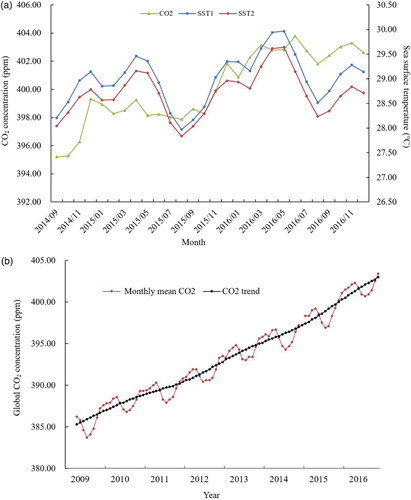
Meanwhile, SST1, SST2 and global SST during the period September-to-December also show a trend of increase from 2014 to 2016. SST1 increased from 28.71°C (2014) to 28.74°C (2015) and 29.07°C (2016); SST2 increased from 28.44°C (2014) to 28.51°C (2015) and 28.64°C (2016); global SST increased from 13.76°C (2014) to 13.90°C (2015) and 13.95°C (2016). In Figure 2, correlation analysis has been conducted between CO₂ concentration and SST1, SST2; the correlation coefficient r for the 30 months of this study is 0.61 for SST1 and 0.54 for SST2 (Figure 2(a,b)). Although the monthly fluctuations and change trends in CO₂ concentration were relatively similar to SST, the annual increase of CO₂ concentration is much more obvious than the increase of SST, which would affect the results of the correlation analysis and caused the correlation coefficient r to not be as high as expected. Both Figure 1(a,b) shows that an intact annual cycle of the wave for the change of CO₂ concentration and SST is from August to next July. Therefore, to alleviate the effect of fast annual increase of CO₂ concentration, the study period has been divided into three parts in August 2015, 2016 and correlation analysis for each annual cycle has been separately conducted. From September 2014 to July 2015, the correlation coefficient r rose to 0.65 for SST1-CO₂ and 0.64 for SST2-CO₂ (Figure 2(c,d)). From August 2015 to July 2016, the correlation coefficient r rose to 0.87 for SST1-CO₂ and 0.85 for SST2-CO₂ (Figure 2(e,f)). From August 2016 to December 2016, the correlation coefficient r rose to 0.94 for SST1-CO₂ and 0.91 for SST2-CO₂ (Figure 2(g,h)). The results show that all the correlations between CO₂ concentration and SST are positive and the correlations between CO₂ and SST1 are always higher than correlations between CO₂ and SST2, which indicate that the SST of the inshore area would affect CO₂ concentration in Indonesia more than the SST of the offshore area.

Figure 2. The correlation between CO₂ concentrations and SST in Indonesia: 2014.09–2016.12, with SST1 (a); 2014.09–2016.12, with SST2 (b); 2014.09–2015.07, with SST1 (c); 2014.09–2015.07, with SST2 (d); 2015.08–2016.07, with SST1 (e); 2015.08–2016.07, with SST2 (f); 2016.08–2016.12, with SST1 (g) and 2016.08–2016.12, with SST2 (h).

Regarding the spatial distribution, Figure 3 shows that the annual SST around Sumatra is always higher than other parts of Indonesia. Meanwhile, the average CO₂ concentration of Sumatra was 399.8 ppm in 2015 and 403.5 ppm in 2016, which was also the highest of the six parts (Table 2). For the data in Table 2, the boundaries of the six regions have been used as masks to obtain CO₂ concentration in these areas. By contrast, the average CO₂ concentration in Java was low, with only 397.8 ppm in 2015 and 401.7 ppm in 2016 (Table 2). Because Java is far away from the equator, Figure 3 shows that the annual SST around Java is also low. The population of Indonesia according to the 2010 national census was 237.64 million (Akbar, Wicaksono, and Dachlan 2012). Fifty-eight percent of the population lives on the island of Java, the world’s most populous island (Afsah and Vincent 2000). Theoretically, the CO₂ concentration in Java should be higher than other regions because of the dense population and active anthropogenic activities. The transportation sector, as one of the most important anthropogenic activities and prolific emitters of Greenhouse Gases (GHGs), accounted for about 28% of US GHG emissions (Morrow et al. 2010). All of the results indicate that the SST as an important factor has a significant impact on the CO₂ concentration in the archipelagic country of Indonesia. Moreover, its annual increase in CO₂ concentration is in accordance with the global concentration increase.

Figure 3. SST around Indonesia in September–December 2014 (a), 2015 all year (b) and 2016 all year (c). Small rectangular with dash line is the boundary of SST1 and big rectangular with dash line is the boundary of SST2.

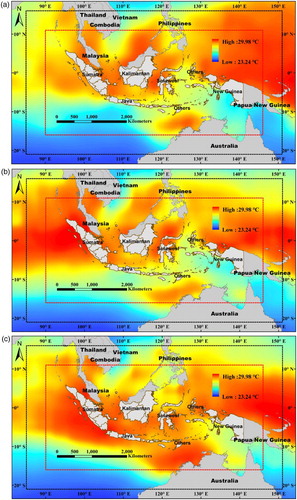
Table 2. Monthly CO₂ concentration in six different parts.

Month	CO2 Concentration (ppm)
	Sumatra	Sulawesi	New Guinea	Java	Kalimantan	Others
2014/09	395.6	395.3	396.5	394.7	394.9	395.2
2014/10	395.1	395.2	396.0	393.8	396.3	395.0
2014/11	398.5	395.6	396.3	394.3	397.8	395.3
2014/12	398.6	399.7	399.8	398.3	400.6	397.1
2015/01	401.0	397.3	399.1	396.9	400.4	396.6
2015/02	398.5	397.1	399.5	397.2	400.1	397.6
2015/03	399.5	397.8	398.6	396.7	398.8	398.3
2015/04	399.3	398.4	399.1	397.0	400.4	398.5
2015/05	398.6	396.7	397.8	397.5	399.1	397.9
2015/06	398.9	396.2	398.5	397.7	398.9	397.4
2015/07	398.4	398.6	398.6	397.3	397.8	398.0
2015/08	399.1	397.7	398.2	396.7	398.4	398.3
2015/09	399.5	398.5	398.6	398.0	398.9	398.8
2015/10	400.4	397.6	397.2	397.8	399.8	398.6
2015/11	400.6	399.4	401.1	399.6	401.1	399.2
2015/12	404.1	400.8	403.1	401.7	403.4	401.1
2016/01	402.0	400.4	400.2	401.3	403.0	398.4
2016/02	403.5	401.0	402.2	401.6	402.5	399.6
2016/03	403.2	403.5	405.6	401.2	403.1	403.1
2016/04	403.9	402.6	403.5	403.0	404.2	400.5
2016/05	404.0	401.4	403.3	400.7	405.0	401.0
2016/06	404.3	403.6	402.4	403.0	404.2	402.3
2016/07	403.8	401.7	400.2	400.7	403.8	401.7
2016/08	405.1	400.0	401.6	402.3	402.7	400.8
2016/09	402.8	403.1	403.3	401.4	403.8	401.1
2016/10	402.8	405.0	402.3	404.1	404.0	402.4
2016/11	404.1	403.5	406.4	401.0	401.5	401.6
2016/12	402.3	398.1	406.6	402.9	404.9	401.6

3.2. Fire hotspots and CO₂ concentration

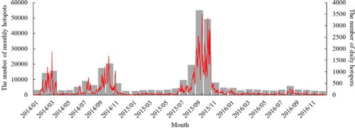
From Thermal Anomalies/Fire images, 83,083 fire hotspots were detected in Indonesia in 2014 and this number increased from 69.35% to 140,699 in 2015. This sudden growth of fire hotspots was caused by the worst forest fire since 1997, burning approximately 261,000 hectares of forests and peatland. While after devastating forest fire there were only 16,454 fire hotspots detected in 2016, which was much lower than  those in other two years. Figure 4 shows that the number of hotspots was greatest in September 2015, at 52,903, and the second largest occurred in October 2015, at 47,094. The number of hotspots detectable in these two months account for 71.05% of all hotspots detected in 2015. On 23 September 2015, the number of hotspots was 3497, the highest daily totals for the three years in the study period. According to Figure 4, three main fires occurred in Indonesia, the first in February–March 2014, the second in September–October 2014 and the last one in September–October 2015. The daily and monthly number of fire hotspots in 2016 showed no evident fluctuation and they were always less than the other two years.

Figure 4. Daily (full line) and monthly (gray column) number of fire hotspots in Indonesia from 2014 to 2016.

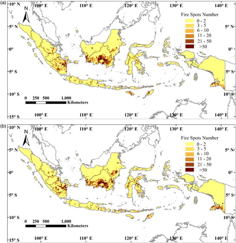
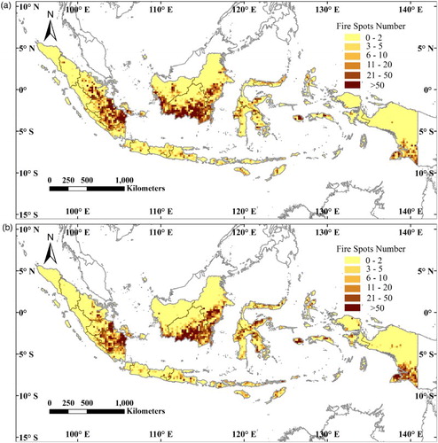
In February–March 2014, Table 3 and results show that most of hotspots were distributed in Sumatra’s middle-east portion (Riau). Fire hotspots in Sumatra accounted for 85.93% of all of the hotspots in February and 91.07% in March. In September–October 2014, Figure 5(a,b) presents most of the hotspots were distributed in the south of Kalimantan (Kalimantan Tengah). Fire hotspots in Kalimantan accounted for 47.96% of all hotspots in September and 47.30% in October. In September–October 2015, most of the hotspots were distributed in south of Kalimantan (Kalimantan Tengah) and southeast of Sumatra (Sumatera Selatan). Fire hotspots in these two islands accounted for 82.92% of all hotspots in September and 73.84% in October. Combining fire hotspots with the land cover of Indonesia, the results indicate that most of the hotspots were distributed in two land cover types, Evergreen Broadleaf Forest and Crop and Natural Vegetation Mosaic. In 2014, hotspots in Evergreen Broadleaf Forest accounted for 63.11% of all hotspots and 19.43% in Crop and Natural Vegetation Mosaic. In 2015, hotspots in Evergreen Broadleaf Forest accounted for 70.51% of all hotspots and in Crop and Natural Vegetation Mosaic accounted for 16.05%. In 2016, hotspots in Evergreen Broadleaf Forest accounted for 51.63% of all hotspots and in Crop and Natural Vegetation Mosaic accounted for 20.69%. This finding demonstrates that a large proportion of hotspots in Indonesia are from forest fire, while crop residue burning also accounts for a certain percentage of hotspots.

Figure 5. Spatial distribution of fire hotspots in Indonesia: September 2014 (a); October 2014 (b); September 2015 (c) and October 2015 (d).

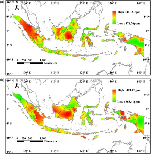
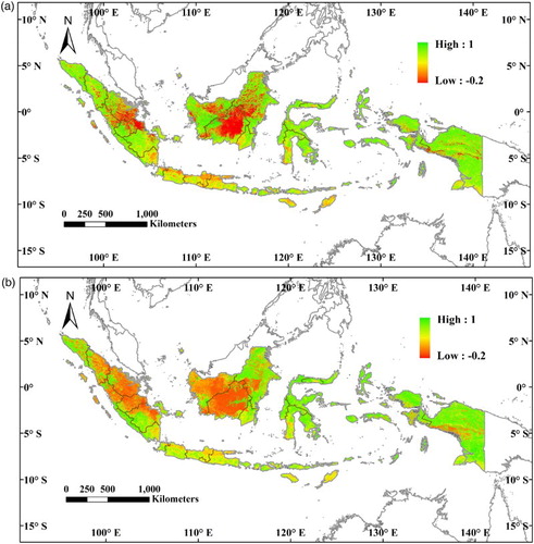
During the most severe forest fire in September and October 2015, the CO₂ concentration in Indonesia only exhibited an obvious rise in September. By contrast, in October it exhibits a sudden decline. Regarding the spatial distribution, Figure 5 shows that in September and October the CO₂ concentration of Kalimantan and Sumatra was higher than in other areas. Meanwhile, via Figures 5(e,f) and 6(c,d), we found that hotspots and CO₂ concentration showed a higher spatial consistency. Although the average CO₂ concentration of Indonesia decreased from 398.6 to 398.3 ppm in October 2015, the CO₂ concentration in Kalimantan and Sumatra increased dramatically in this month. In Kalimantan, CO₂ concentration increased from 399.5 to 400.4 ppm and in Sumatra the CO₂ concentration increased from 398.9 to 399.8 ppm (Table 2), which is totally different from the left four parts of Indonesia and the left four parts presented a trend of decrease. The still ongoing forest fire is assumed to be the main reason for the CO₂ concentration increase in Kalimantan and Sumatra in October 2015. Table 3 shows that in this month there were still 16,388 fire hotspots on Sumatra and 18,385 on Kalimantan.

Table 3. Number of fire hotspots in different islands.

Islands	2014/02	2014/03	2014/09	2014/10	2015/09	2015/10
Sumatra	10,475	12,325	4110	4627	19,914	16,388
Sulawesi	98	165	822	1489	2509	3415
New Guinea	29	25	904	1452	2853	4680
Java	28	106	674	493	758	808
Kalimantan	1386	708	7400	8662	23,923	18,385
Others	174	205	1519	1590	2946	3418
All	12,190	13,534	15,429	18,313	52,903	47,094

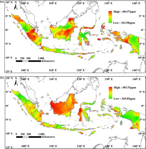
Since the CO₂ data after September 2014 are available, the CO₂ concentration change during the forest fires in September and October 2014 has also been analyzed. Regarding the spatial distribution, the distribution map in Figure 6(b) shows that in October the CO₂ concentration in Kalimantan was much higher than in other areas. Unlike 2015, the CO₂ concentration in Indonesia did not exhibit a decreasing trend from September to October; instead, the concentration increased very slightly from 395.2 to 395.3 ppm, while the CO₂ concentration in Kalimantan rose steeply from 394.9 to 396.3 ppm. By contrast, CO₂ concentration in the left five parts of Indonesia clearly decreased, including in Sumatra, where it declined from 395.6 to 395.1 ppm. As previously mentioned, hotspots were mainly distributed in Kalimantan during the forest fire in September–October 2014, and the CO₂ emissions from forest fires are regarded as an important factor in the CO₂ concentration increase in Kalimantan.

Figure 6. Spatial distribution of CO₂ concentration in Indonesia: September 2014 (a); October 2014 (b); September 2015 (c) and October, 2015 (d).

By analyzing the CO₂ concentration change during the two forest fires in 2014 and 2015, we concluded that unlike SST, forest fires cannot induce an obvious CO₂ increase over the whole country because the six parts of Indonesia are separated by the ocean and their geographical locations are relatively independent. However, CO₂ concentration presented a trend of rise in corresponding islands during the occurrence of forest fire, and CO₂ concentration increased in Kalimantan during the forest fire in 2014 and CO₂ concentration increased on Kalimantan and Sumatra during the forest fire in 2015.

3.3. Vegetation and CO₂ concentration

The vegetation found in Indonesia is typical of the tropics, and forests cover approximately 60% of the country. Figure 7(a) shows that vegetation indices were very stable and smooth during the study period except in October 2015. Because of the high forest coverage rate, the average NDVI and EVI in 2014–2016 were relatively higher than in other countries, with values of 0.77 and 0.49, respectively. Figure 7(a) shows that the wave of vegetation indices is entirely different from CO₂ concentration. Our analysis did not uncover any correlations between vegetation indices and CO₂ concentration; by contrast, the correlation coefficient r between NDVI and EVI is 0.83 (Figure 7(b)). Guo et al. (“Spatial Distribution of Greenhouse Gas,” 2013) have found that in East Asia’s arid and semi-arid regions, the correlation coefficient between annual CO₂ concentration and annual NDVI can reach up to 0.87. CO₂ concentration data of their research were obtained from Scanning Imaging Absorption spectroMeter for Atmospheric CHartographY (SCIAMACHY) and GOSAT. We assume that the following reasons explain why there is no correlation between vegetation indices and CO₂ concentration. Firstly, Indonesia is an archipelago country, and, hence, SST plays a crucial role in CO₂ concentration; second, the location of Indonesia is around the equator and there are not four distinctive seasons in this country. Lastly, the vegetation is mainly evergreen broadleaf and the vegetation indices of this kind vegetation are stable throughout the entire year. Unlike the vegetation cover on frigid zone and temperate zone, the photosynthesis and respiration of the vegetation in Indonesia are more steady all through the year.

Figure 7. Monthly CO₂ concentration and vegetation indices, NDVI and EVI (a); correlation between NDVI and EVI (b).

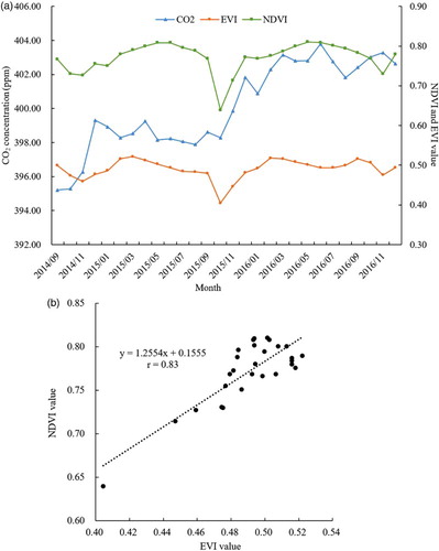
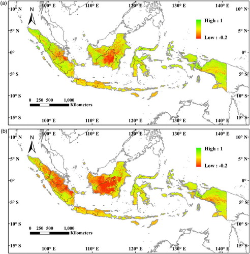
In October 2015, forest fire caused a sudden decrease of NDVI in Indonesia from 0.77 to 0.64 and a decrease of EVI from 0.48 to 0.40. Comparing the six parts of the country, NDVI and EVI in Kalimantan and Sumatra decreased even more clearly. NDVI decreased from 0.81 to 0.64 in Kalimantan and from 0.78 to 0.52 in Sumatra. EVI decreased from 0.50 to 0.40 in Kalimantan and from 0.50 to 0.35 in Sumatra. Figure 8 also indicates that the forest fire induced a decline in vegetation indices in Kalimantan and Sumatra. Vegetation indices in the other four parts did not exhibit any abnormal changes, but the vegetation indices in Java were always lower, and the monthly fluctuations were more evident than on other islands. This finding is observed because some 60% of the country’s cultivated land is in Java. The vegetation indices of farmland are much lower than in tropic forests and the farming activities could also affect the fluctuations of vegetation indices in Java.

Figure 8. NDVI of Indonesia in September (a) and October (b) 2015; EVI of Indonesia in September (c) and October (d) 2015.

4. Conclusions

CO₂ concentration changes in Indonesia from September 2014 to December 2016 have been analyzed using OCO-2 Level 2 products. Via other remote-sensing data, the relationship between CO₂ concentration changes and three influencing factors (SST, forest fire and vegetation) is also presented in this study. As an archipelago country, SST directly affects the CO₂ concentration in Indonesia and its effect is more crucial than the other factors. CO₂ concentration in Indonesia showed an annual increase that is consistent with the global increase discovered by GOSAT project (Figure 1). At the same time, global SST and SST around Indonesia also show an increasing trend. Although the forest fires in September–October 2014 and 2015 did not induce an obvious rising of CO₂ over the whole country, both CO₂ concentration in corresponded islands show a trend of increases during the forest fires. CO₂ concentration increased in Kalimantan during the occurrence of forest fire in September–October 2014 and CO₂ concentration increased in Kalimantan and Sumatra during occurrence of forest fire in September–October 2015. MODIS hotspots also prove that forest fires in September–October 2014 were mainly distributed in Kalimantan, and forest fires in September–October 2015 were primarily distributed in Kalimantan and Sumatra. We assume that the greenhouse gas emitted from forest fire is an important source to lead to CO₂ increase in these regions. Since only two fires have been studied in this research and in the future more fire cases in Indonesia need to be analyzed to obtain the final conclusion. The vegetation indices in Indonesia are stable and show no correlation with CO₂ changes because of the special geographic location, climate conditions and vegetation types in Indonesia. Meanwhile, the vegetation index declined rapidly during the devastating forest fire in September–October 2015. This study shows that unlike GOSAT, which provides limited data on Indonesia, OCO-2 can effectively facilitate CO₂ concentration research at a regional scale, such as Indonesia and even smaller areas.

Meanwhile, this study also fills in the gap that no research exists on using greenhouse gas monitoring satellites to analyze CO₂ concentration changes at a regional scale. The results and influencing factors of this study are only applicable for island countries around the equator. Other studies should consider different factors according to the conditions in the study area. Before NASA releases OCO-2 Level 3 products (Global X_CO2), this study proposes an effective method to use Level 2 products (Orbit granules of geolocated X_CO2 products) to analyze CO₂ concentration changes. The data of OCO-2 are only available from September 2014, and CO₂ concentration changes are a long, slow and complicated process; therefore, we hope that in the future more researches will be carried out by greenhouse gas monitoring satellites. And combining OCO-2 with GOSAT, greenhouse gas monitoring satellites will also become powerful tools to improve predictions of future atmospheric CO₂ increases and their impact on the Earth's climate.

Acknowledgements

We are grateful to OCO-2 project at the Jet Propulsion Laboratory, California Institute of Technology, and obtained from the OCO-2 data archive maintained at the NASA Goddard Earth Science Data and Information Services Center. We also thank the GOSAT Project, NASA and NOAA for the use of their data in this study.

Disclosure statement

No potential conflict of interest was reported by the authors.

References

- Afsah, S., and J. R. Vincent. 2000. Asia's Clean Revolution: Industry, Growth and the Environment. Yorkshire: Greenleaf Publishing in association with GSE Research.
- Akbar, A., B. Wicaksono, and E. G. Dachlan. 2012. “Maternal Mortality and Its Mainly Possible Causepre-Eclampsia/Eclampsia in Developing Country (Surabaya-Indonesia as Themodel).” Pregnancy Hypertension 2 (3): 184. doi: 10.1016/j.preghy.2012.04.019
- Basu, S., S. Guerlet, A. Butz, S. Houweling, O. Hasekamp, I. Aben, P. Krummel, et al. 2013. “Global CO2 Fluxes Estimated from GOSAT Retrievals of Total Column CO2.” Atmospheric Chemistry and Physics 13 (17): 8695–8717. doi: 10.5194/acp-13-8695-2013
- Bond-Lamberty, B., S. D. Peckham, D. E. Ahl, and S. T. Gower. 2007. “Fire as the Dominant Driver of Central Canadian Boreal Forest Carbon Balance.” Nature 450 (7166): 89–92. doi: 10.1038/nature06272
- Cai, S., D. Liu, D. Sulla-Menash, and M. A. Friedl. 2014. “Enhancing MODIS Land Cover Product with a Spatial-Temporal Modeling Algorithm.” Remote Sensing of Environment 147 (18): 243–255. doi: 10.1016/j.rse.2014.03.012
- Canadell, J. G., C. Le Quéré, M. R. Raupach, C. B. Field, E. T. Buitenhuis, P. Ciais, T. J. Conway, N. P. Gillett, R. A. Houghton, and G. Marland. 2007. “Contributions to Accelerating Atmospheric CO2 Growth from Economic Activity, Carbon Intensity, and Efficiency of Natural Sinks.” Proceedings of the National Academy of Sciences of the United States of America 104(47): 18866–18870. doi: 10.1073/pnas.0702737104
- Crisp, D. 2014. “Retrieving CO2 from Orbiting Carbon Observatory-2 (OCO-2) Spectra.” Paper presented at the 13th International HITRAN Conference, Cambridge, MA, June 23–25.
- Crisp, D., R. M. Atlas, F. M. Breon, L. R. Brown, J. P. Burrows, P. Ciais, B. J. Connor, et al. 2004. “The Orbiting Carbon Observatory (OCO) Mission.” Advances in Space Research 34 (4): 700–709. doi: 10.1016/j.asr.2003.08.062
- Fensholt, R., and I. Sandholt. 2005. “Evaluation of MODIS and NOAA AVHRR Vegetation Indices with in Situ Measurements in a Semi-arid Environment.” International Journal of Remote Sensing 26: 2561–2594. doi: 10.1080/01431160500033724
- Frankenberg, C., R. Pollock, R. A. M. Lee, R. Rosenberg, J. F. Blavier, D. Crisp, C. W. O’Dell, et al. 2014. “The Orbiting Carbon Observatory (OCO-2): Spectrometer Performance Evaluation Using Pre-launch Direct Sun Measurements.” Atmospheric Measurement Techniques Discussions 7 (1): 7641–7670. doi: 10.5194/amtd-7-7641-2014
- Giglio, L., J. Descloitres, C. O. Justice, and Y. J. Kaufman. 2003. “An Enhanced Contextual Fire Detection Algorithm for MODIS.” Remote Sensing of Environment 87 (2-3): 273–282. doi: 10.1016/S0034-4257(03)00184-6
- Guo, M., X. F. Wang, J. Li, H. Wang, and H. Tani. 2013. “Examining the Relationships Between Land Cover and Greenhouse Gas Concentrations Using Remote-Sensing Data in East Asia.” International Journal of Remote Sensing 34: 4281–4303. doi: 10.1080/01431161.2013.775535
- Guo, M., X. F. Wang, J. Li, K. P. Yi, G. S. Zhong, H. M. Wang, H. Tani, O. Schneising, and M. Reuter. 2013. “Spatial Distribution of Greenhouse Gas Concentrations in Arid and Semi-Arid Regions: A Case Study in East Asia.” Journal of Arid Environments 91 (4): 119–128. doi: 10.1016/j.jaridenv.2013.01.001
- Justice, C. O., L. Giglio, S. Korontzi, J. Owens, J. T. Morisette, D. Roy, J. Descloitres, S. Alleaume, F. Petitcolin, and Y. Kaufman. 2002. “The MODIS Fire Products.” Remote Sensing of Environment 83: 244–262. doi: 10.1016/S0034-4257(02)00076-7
- Kawasaki, M., H. Yoshioka, N. B. Jones, R. Macatangay, D. W. T. Griffith, S. Kawakami, H. Ohyama, et al. 2012. “Usability of Optical spectrum Analyzer in Measuring Atmospheric CO2 and CH4 Column Densities: Substantiation with FTS and Aircraft Profiles In Situ.” Atmospheric Measurement Techniques Discussions 5: 4099–4121. doi: 10.5194/amtd-5-4099-2012
- Kim, Y., J. S. Kimball, K. Didan, and G. M. Henebry. 2014. “Response of Vegetation Growth and Productivity to Spring Climate Indicators in the Conterminous United States Derived from Satellite Remote Sensing Data Fusion.” Agricultural and Forest Meteorology 194: 132–143. doi: 10.1016/j.agrformet.2014.04.001
- Kimball, B. A., J. R. Mauney, F. S. Nakayama, and S. B. Idso. 1993. “Effects of Increasing Atmospheric CO2 on Vegetation.” Vegetatio 104-105: 65–75. doi: 10.1007/BF00048145
- Konovalov, I. B., E. V. Berezin, P. Ciais, G. Broquet, M. Beekmann, J. Hadji-Lazaro, C. Clerbaux, M. O. Andreae, J. W. Kaise, and E. D. Schulze. 2014. “Constraining CO2 Emissions from Open Biomass Burning by Satellite Observations of Co-emitted species: A Method and Its Application to Wildfires in Siberia.” Atmospheric Chemistry and Physics Discussions 14: 3099–3168. doi: 10.5194/acpd-14-3099-2014
- Landschützer, P., N. Gruber, D. C. E. Bakker, and U. Schuster. 2014. “Recent Variability of the Global Ocean Carbon Sink.” Global Biogeochemical Cycles 28: 927–949. doi: 10.1002/2014GB004853
- Lin, S., N. J. Moore, J. P. Messina, M. H. Devisser, and J. Wu. 2012. “Evaluation of Estimating Daily Maximum and Minimum Air Temperature with MODIS Data in East Africa.” International Journal of Applied Earth Observation and Geoinformation 18 (1): 128–140. doi: 10.1016/j.jag.2012.01.004
- Loveland, T. R., and A. S. Belward. 1997. “The International Geosphere Biosphere Programme Data and Information System Global Land Cover Data Set (DISCover).” Acta Astronautica 41: 681–689. doi: 10.1016/S0094-5765(98)00050-2
- Lubowski, R. N., A. J. Plantinga, and R. N. Stavins. 2006. “Land-use Change and Carbon Sinks: Econometric Estimation of the Carbon Sequestration Supply Function.” Journal of Environmental Economics and Management 51 (2): 135–152. doi: 10.1016/j.jeem.2005.08.001
- Manduchi, G. 2010. “Commonalities and Differences Between MDSplus and HDF5 Data Systems.” Fusion Engineering and Design 85: 583–590. doi: 10.1016/j.fusengdes.2010.03.055
- Morrow, W. R., K. S. Gallagher, G. Collantes, and H. Lee. 2010. “Analysis of Policies to Reduce Oil Consumption and Greenhouse-gas Emissions from the US Transportation Sector.” Energy Policy 38 (3): 1305–1320. doi: 10.1016/j.enpol.2009.11.006
- OCO-2 Data Product User’s Guide. 2015. “Operational L1 and L2 Data Versions 7 and 7R.” National Aeronautics and Space Administration, Jet Propulsion Laboratory California Institute of Technology Pasadena, California.
- Oguma, H., I. Morino, H. Suto, Y. Yoshida, N. Eguchi, A. Kuze, and T. Yokota. 2011. “First Observations of CO2 Absorption spectra Recorded in 2005 Using an Airship-Borne FTS (GOSAT TANSO-FTS BBM) in the SWIR Spectral Region.” International Journal of Remote Sensing 32 (24): 9033–9049. doi: 10.1080/01431161.2010.535864
- Poulter, B., D. C. Frank, E. L. Hodson, and N. E. Zimmermann. 2011. “Impacts of Land Cover and Climate Data Selection on Understanding Terrestrial Carbon Dynamics and the CO2 Airborne Fraction.” Biogeosciences (Online) 8: 2027–2036. doi: 10.5194/bg-8-2027-2011
- Prasad, P., S. Rastogi, and R. P. Singh. 2014. “Study of Satellite Retrieved CO2 and CH4 Concentration Over India.” Advances in Space Research 54 (9): 1933–1940. doi: 10.1016/j.asr.2014.07.021
- Quéré, C. L., M. R. Raupach, J. G. Canadel, and G. Marland. 2009. “Trends in the Sources and Sinks of Carbon Dioxide.” Nature Geoscience 2 (12): 831–836. doi: 10.1038/ngeo689
- Reynolds, R. W., and D. C. Marsico. 1993. “An Improved Real-time Global Sea Surface Temperature Analysis.” Journal of Climate 6 (1): 114–119. doi: 10.1175/1520-0442(1993)006<0114:AIRTGS>2.0.CO;2
- Reynolds, R. W., and T. M. Smith. 1994. “Improved Global Sea Surface Temperature Analyses Using Optimum Interpolation.” Journal of Climate 7 (6): 929–948. doi: 10.1175/1520-0442(1994)007<0929:IGSSTA>2.0.CO;2
- Ryan, M. G. 1991. “Effects of Climate Change on Plant Respiration.” Ecological Applications 1 (2): 157–167. doi: 10.2307/1941808
- Saito, R., P. K. Patra, N. Deutscher, D. Wunch, K. Ishijima, V. Sherlock, T. Blumenstock, et al. 2012. “Latitude-time Variations of Atmospheric Column-Average dry air Mole Fractions of CO2, CH4 and N2O.” Atmospheric Chemistry and Physics Discussions 12: 5679–5704. doi: 10.5194/acpd-12-5679-2012
- Salazar, N. B. 2014. Encyclopedia of Global Archaeology. Berlin: Springer.
- Sibson, R. 1981. Interpreting Multivariate Data. Hoboken, NJ: Wiley Press.
- Siegenthaler, U., and J. L. Sarmiento. 1993. “Atmospheric Carbon Dioxide and the Ocean.” Nature 365: 119–125. doi: 10.1038/365119a0
- Solomon, S., D. Qin, M. Manning, Z. Chen, M. Marquis, K. B. Averyt, M. Tignor, and H. L. Miller. 2014. Contribution of Working Group I to the Fourth Assessment Report of the Intergovernmental Panel on Climate Change, 2007. Cambridge: Cambridge University Press.
- Stocker, B. D., K. Strassmann, and F. Joos. 2010. “Sensitivity of Holocene Atmospheric CO2 and the Modern Carbon Budget to Early Human Land Use: Analyses with a Process-based Model.” Biogeosciences Discussions 7 (1): 921–952. doi: 10.5194/bgd-7-921-2010
- Taylor, T. E., C. W. O’Dell, C. Frankenberg, P. T. Partain, H. Q. Cronk, A. Savtchenko, R. R. Nelson, et al. 2016. “Orbiting Carbon Observatory-2 (OCO-2) Cloud Screening Algorithms: Validation Against Collocated MODIS and CALIOP Data.” Atmospheric Measurement Techniques 9: 973–989. doi: 10.5194/amt-9-973-2016
- Viironen, K., S. F. Sánchez, E. Marmol-Queraltó, J. Iglesias-Páramo, D. Mast, R. A. Marino, D. Cristóbal-Hornillos, et al. 2012. “Spatially Resolved Properties of the Grand-Design Spiral Galaxy UGC 9837: A Case for High-Redshift 2-D Observations.” Astronomy and Astrophysics 538: A144. doi: 10.1051/0004-6361/201016347
- Yoshida, Y., Y. Ota, N. Eguchi, N. Kikuchi, K. Nobuta, H. Tran, I. Morino, and T. Yokota. 2010. “Retrieval Algorithm for CO2 and CH4 Column Abundances from Short-wavelength Infrared Spectral Observations by the Greenhouse Gases Observing Satellite.” Atmospheric Measurement Techniques Discussions 3 (6): 4791–4833. doi: 10.5194/amtd-3-4791-2010
- Yoshimi, K., K. Hiroshi, T. Shin, H. Kohtaro, M. Hiroshi, K. Misako, and G. Lei. 2006. “Satellite-based High-Resolution Global optimum Interpolation Sea Surface Temperature Data.” Journal of Geophysical Research Atmospheres 111: 285–293.