The spatiotemporal patterns of sea ice in the Bohai Sea during the winter seasons of 2000–2016

ABSTRACT

In this study, sea ice thickness (SIT) and sea ice extent (SIE) in the Bohai Sea from 2000 to 2016 were investigated. A surface heat balance equation was applied to calculate SIT using ice surface temperatures estimated from the Moderate Resolution Imaging Spectroradiometer (MODIS) data with input from air temperature and wind speed from reanalyzing weather data. No trend was found in SIT during 2000–2016. The mean SIT and SIE during this period were 5.58±0.86 cm and 23×10³±8×10³ km², respectively. The largest SIT and SIE periods were observed during the second half of January and the first half of February, respectively. The Spearman correlation coefficient between mean ice thickness and average air temperature from 21 automatic weather stations around the Bohai Sea was –0.94 (P < .005), and the coefficient between median ice extent and negative accumulated temperature was –0.503 (P < .001). The rate of increase in air temperature around the Bohai Sea is 0.271°C per decade in winter for 1979–2016 (P < .05), which is much lower than that in northern polar area (0.648°C per decade). This rate has not resulted in a decreasing trend in SIT and SIE for the past 16 years in the Bohai Sea.

KEYWORDS:

• Sea ice
• the Bohai Sea
• global warming
• ice thickness
• ice extent

1. Introduction

Sea ice is an important component of the climate system. It can greatly influence the exchange of heat, energy, mass, and momentum between the atmosphere and ocean (Dieckmann and Hellmer 2010). Satellite observations have played a pivotal role in sea ice studies. Sea ice thickness (SIT) is crucial for the quantitative understanding of key physical processes in ice-covered waters. For example, it is important for understanding the heat flux between ocean and atmosphere, the mass balance of sea ice, as well as ocean circulation in Polar Regions. SIT is usually obtained from in situ measurements, ship-based observations, and submarine or moored upward-looking sonar measurement. However, these observations are time consuming and spatially limited.

Satellite remote sensing is a powerful tool for monitoring ice thickness over larger areas. A commonly used sensor for estimating thickness of relatively thick ice is satellite altimeter. Observations are augmented with sea ice freeboard (i.e. the part of the ice above water level) and snow layer thickness to calculate SIT based on Archimedes’ law. Sources of satellite altimeter data include the laser altimeter onboard the Ice, Cloud, and land Elevation Satellite (ICESat) and a few radar altimeters onboard the European Remote Sensing (ERS-1/2) satellites (Laxon, Peacock, and Smith 2003), Envisat satellite altimeter (Giles, Laxon, and Ridout 2008), and CryoSat-2 (Kurtz, Galin, and Studinger 2014; Laxon et al. 2013). However, errors in freeboard estimates by altimeters may induce large uncertainties when ice thickness is less than 1 m (Laxon et al. 2013; Zwally et al. 2008). Therefore, satellite altimeter data are more suitable for detection of thick ice (greater than 40 cm). Synthetic aperture radar (SAR) data from dual frequency or dual polarization have been employed to estimate SIT of different ice types (Kim, Kim, and Hwang 2012; Nakamura et al. 2005). However, SAR does not provide the sufficiently wide swath and the high revisit frequency required for operational monitoring.

Thin ice thickness (less than 0.5 m) can be estimated by optical and thermal infrared (TIR) imagery. The approach involves using a heat balance equation with input parameters such as surface temperature and albedo that can be obtained from different channels on the same platform (Yu and Rothrock 1996). Another approach, adopted in the RADARSAT Geophysical Processor System (RGPS) at the Alaska SAR Facility, involves tracking the area changes of Lagrangian cells over time. From this product, SIT is estimated on the basis of freezing degree days, area change history, and ridging observations (Yu and Lindsay 2003). Passive microwave data from 37 GHz channels have also been used to retrieve SIT of less than approximately 0.5 m using empirical relations between thickness and a radiometric measurement such as the polarization ratio (Martin et al. 2004). The passive L-band radiometer (1.4 GHz) onboard the Soil Moisture and Ocean Salinity mission (SMOS) satellite is used to retrieve thickness between a few centimeters to approximately 1 m, depending on ice temperature and salinity (Huntemann et al. 2014; Kaleschke et al. 2016; Tian-Kunze et al. 2014). Uncertainty of the SIT retrieval from passive microwave data is linked to tuning coefficients in empirical equations, the heterogeneity of the contents of the footprint of the satellite observations, the geolocations’ accuracy of the data, and relevant meteorological conditions. For instance, SMOS-based SIT retrieval is only used in cold periods, with high (almost 100%) sea ice concentration, and is heavily impeded by the presence of clouds.

The Bohai Sea (37°-41°N, 117°-123°E), located off the northeast coast of China, is the southernmost region in the Northern Hemisphere where seasonal sea ice occurs annually from December to February with possible duration into March. The ice thickness is usually less than 50 cm (Li and Wang 2001). Historically, the Bohai sea ice has caused serious damage to marine transportation, offshore oil platforms, the fishing industry, and coastal construction (Yang 2000). Operational sea ice monitoring and forecasting have both been carried out by the National Marine Environment Forecasting Center (Bai and Wu 1998; Guo et al. 2006). Different tools have been used to monitor SIT and SIE in the Bohai Sea, including the Advanced Very High Resolution Radiometer (AVHRR) satellite, the Moderate Resolution Imaging Spectroradiometer (MODIS) satellite, the Thermal Mapper (TM), the Geostationary Ocean Color Imager (GOCI) data, the Huanjing 1 (HJ-1) charge coupled device (CCD) data, and the Haiyang 1A (HY-1A) CCD imagery (Karvonen et al. 2017; Liu et al. 2000; Liu et al. 2015; Liu, Sheng, and Zhang 2016; Luo et al. 2004; Ning et al. 2009; Shi et al. 2016; Su et al. 2015; Su and Wang 2012; Su, Wang, and Yang 2012; Zeng et al. 2016). These studies have contributed to the understanding of sea ice processes and air–sea interactions, especially for the purpose of disaster reduction and emergency management caused by sea ice.

So far, there have been no long-term studies on the spatiotemporal distributions and variations of sea ice in the Bohai Sea. Therefore, the objective of this study is twofold. First is to examine the spatiotemporal patterns of sea ice (i.e. SIT and SIE) from 2000 to 2016 using surface heat balance equation with input from MODIS data. Second is to analyze the relationship between SIT and SIE and air temperature recorded by automatic weather stations (AWS). This is performed to explore the impact of global warming trends in the Bohai Sea region (mid-latitude region) on SIT and SIE.

2. Study area

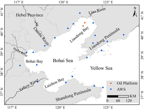
The Bohai Sea is a shallow inland sea within the larger China Sea with an average depth of only 18 m, and connected with the Yellow Sea through the Bohai Strait (Figure 1). It is surrounded by the Liaodong and Shandong Peninsula and contains four major water bodies: Liaodong Bay in the north, Bohai Bay in the west, Laizhou Bay in the south, and the Central Area in the center. More than 40 rivers flow into the Bohai Sea, among which four major are the Yellow River, Haihe River, Luanhe River, and Liaohe River. The Bohai Sea is seasonally covered by ice from late December to the end of March. The thickness of undeformed sea ice can reach 50 cm in a severely cold winter (Li and Wang 2001), and the ice extent appears to reach its maximum extent in early February (Bai et al. 1999). The surface salinity in the Bohai Sea, especially in the coastal regions, varies between 26‰ and 33‰ with great spatiotemporal variations due to river discharge, precipitation, evaporation, and currents (Song et al. 2013; Wu et al. 2004). Spatial variation of surface salinity induces different freezing temperatures, which results in different sea ice physical properties.

Figure 1. Location of the Bohai Sea and distribution of automatic weather stations.

3. Dataset

Night-acquired MODIS data and ERA-Interim reanalysis data from the European Centre for Medium-Range Weather Forecasts (ECMWF) from 2000 to 2016 are used for ice thickness calculations. Meteorological data observed by AWS are used for the analysis of relationship between SIE and SIT and air temperature. Ice thickness data from in situ observations at two offshore oil platforms (JZ9–3 and JZ20–2) in Liaodong Bay were obtained from published studies for ice thickness validation (Shi et al. 2016; Zeng et al. 2016). All data were transformed into the Universal Transverse Mercator (UTM) projection. The map projection is referenced to the WGS-84 ellipsoid datum with zone 51N.

3.1. MODIS data

MODIS is a key instrument aboard both Terra satellite (launched in December 1999) with observations from February 2000 to the present and Aqua satellite (launched in May 2002) with observations from June 2002 to the present. The sensor can achieve global coverage every 1–2 days. It has 36 spectral bands, which covers the visible and infrared wavelengths from approximately 0.4 to 14.4 µm. Two bands are imaged at a nominal spatial resolution of 250 m at nadir, five bands at 500 m, and the remaining bands at 1000 m.

MODIS TIR band data are mainly used to retrieve land surface temperature, which can be used to estimate surface energy and ice sheet balance at local and global scales. These data are used in the present study to retrieve sea ice surface temperature (IST) which is required for ice thickness estimation. The daily MODIS level 1 radiance data from the TIR bands 31 (centered at 11.03 μm) and 32 (centered at 12.02 μm), along with Geolocation data with land/sea mask and solar and view angle information (MOD03 and MYD03) were downloaded from NASA’s Atmosphere Archive and Distribution System (LAADS) (http://ladsweb.nascom.nasa.gov/data/search.html). The spatial resolution of all data is 1000 m. The MOD021 data from the Terra satellite and MYD021KM data from the Aqua satellite were acquired from 2000 to 2016 and from 2003 to 2016, respectively. Approximately 80 MODIS images from both satellites can completely cover the Bohai Sea in one month. Only cloud-free images were used (about one-quarter of the available images). For each winter (December, January, and February), approximately 40–60 MODIS images were used for ice thickness estimation. The number of MODIS images with minimum cloud cover in each winter is shown in Table 1. IST and ice thickness calculations are based on these images.

Table 1. The number of MODIS images in each winter.

Year	Numbers	Year	Numbers
2000–2001^a	13	2008–2009	54
2001–2002	19	2009–2010	50
2002–2003	49	2010–2011	52
2003–2004	52	2011–2012	46
2004–2005	46	2012–2013	40
2005–2006	46	2013–2014	44
2006–2007	59	2014–2015	51
2007–2008	52	2015–2016	49

^a2000–2001 denotes December 2000, January 2001, and February 2001. The remainder can be deduced by analogy. Before June 2003, only Terra MODIS data are available; after June 2003, MODIS data from both Terra and Aqua satellites are available.

3.2. Meteorological data

It is not possible to obtain gridded in situ observations of wind speed and air temperature data used for ice thickness estimates over the Bohai Sea. We can only get point data from AWS. Therefore, ERA-Interim reanalysis data were downloaded from ECMWF (http://apps.ecmwf.int/datasets/data/interim-full-daily/). The data included 2-m dewpoint temperature as well as air temperature and 10-m wind speed with a spatial resolution of 0.125°. The latter is corrected to a corresponding 2-m wind speed (Adams et al. 2013). The wind speed and air temperature are interpolated into raster data with a resolution of 1000 m, which is consistent with the spatial resolution of MODIS data.

Daily air temperature from 21 AWS around the Bohai Sea was downloaded from the Climatic Data Center of the National Meteorological Information Center at the China Meteorological Administration (http://data.cma.cn/). The locations of the 21 AWS are illustrated in Figure 1. The observation data were collected from 1951 to 2016. The air temperature is used to explore a possible global warming trend over a longer time series and to explore possible link between this trend and ice thickness and extent in the Bohai Sea.

3.3. Ice thickness data from in situ observations

Ice thickness estimates from sea ice surface heat balance equation should be validated when used for long-term analysis. However, it is difficult to obtain in situ observation data. In this study, data from two offshore oil platforms in Liaodong Bay in the winter season of 2009–2010 and 2012–2013 were obtained from published studies (Shi et al. 2016; Zeng et al. 2016) for validation. The locations of the two offshore oil platforms are shown in Figure 1. The in situ observations were made according to World Meteorological Organization standards and guidelines for sea ice. Detailed descriptions can be found in Zeng et al. (2016).

4. Methods

4.1. The sea ice surface heat balance equation

In cold quiescent conditions, the growth of level and undeformed sea ice is determined by the energy balance equation. A one-dimensional surface energy balance equation is used to derive the ice thickness distribution. The major assumptions in the model are that the heat flux through the ice is equal to the heat flux between the ice surface and atmosphere, and the ice temperature profile is linear in the vertical direction. The model was verified using in situ observations (Nakawo and Sinha 1981) and results from a theoretical study (Maykut 1982). In the absence of shortwave radiation, a simple linear approximation of this balance is described by the following equation (Yu and Rothrock 1996).(1) $(F_l^{\mathrm{u}\mathrm{p}}+F_l^{\mathrm{d}\mathrm{n}}+F_s+F_e)+F_c=F_t+F_c=0,$(1) where $F_l^{\mathrm{u}\mathrm{p}}$ and $F_l^{\mathrm{d}\mathrm{n}}$ are upward and downward longwave radiative fluxes, $F_s$ is the sensible heat flux and $F_e$ is the latent heat flux, and $F_c$ is the surface conductive heat flux. The five parameters can be estimated using the following equations.(2) $F_l^{\mathrm{u}\mathrm{p}}=\epsilon \sigma T_s^4,$(2) (3) $F_l^{\mathrm{d}\mathrm{n}}={\epsilon }^{\ast }\sigma T_a^4,$(3) (4) $F_s={\rho }_a{c}_p{C}_{s}u(T_a-T_s),$(4) (5) $F_e={\rho }_{a}L{C}_{e}u(f{e}_{sa}-e_{s0}),$(5) where $\epsilon$ is the sea ice thermal emissivity (assumed to be constant at 0.98), $\sigma$ is the Stefan–Boltzmann constant with the value of 5.67 × 10⁻⁸W m⁻² K⁻⁴, $T_s$ is IST (estimated from MODIS data), and ${\epsilon }^{\ast }$ is the effective emissivity for the atmosphere, estimated as ${\epsilon }^{\ast }=0.7855(1+0.2232C^{2.75})$, where $C$ is the fractional cloud cover. $T_a$ is air temperature at 2 m above the ice surface (estimated from ERA-Interim data), ${\rho }_a$ is air density with the value of 1.3 kg m⁻³, $c_p$ is specific heat of air at constant pressure with the value of 1006 J kg⁻¹ K⁻¹, $C_s$ and $C_e$ are bulk transfer coefficients for heat and evaporation with the values of 0.03 for thin ice, $L$ is latent heat of vaporization (2.49 × 10⁶ J kg⁻¹), $u$ is wind speed at 2 m above the ice surface (estimated from ERA-Interim data), $e_{sa}$ is saturation vapor pressure which depends on air temperature, $f$ is the relative humidity, assumed to be 90%, $f{e}_{sa}$ is surface water vapor pressure, and $e_{s0}$ is saturation vapor pressure at the surface.

It is assumed that temperature gradients in ice are linear, so the conductive heat flux can be estimated as(6) $F_c=\gamma (T_w-T_s)=\frac{k_i{k}_s}{k_s{h}_i+k_i{h}_s}(T_w-T_s),$(6) where $\gamma$is the thermal conductance of the snow/ ice sheet, $k_i$ and $k_s$ are the thermal conductivities of ice and snow, which are assumed to be 2.304 and 0.3097 W m⁻¹ K⁻¹, respectively, $h_i$ is SIT, $h_s$ is snow depth, $T_w$ is the freezing temperature of seawater, approximated as $T_w=-0.054S_w$, where $S_w$ is seawater salinity, which is assumed to be 30.0‰ for the Bohai Sea. The coefficients and parameters used in the equations are based on Zeng et al. (2016).

4.2. Ice surface temperature calculation

The split-window algorithm is used to estimate the IST. This has been a widely used technique to calculate land, sea and IST from satellite TIR observations under clear sky conditions. The accuracy of the IST product using MODIS data is reported to be within 1.2–1.3 K in both the Arctic and Antarctic regions (Hall et al. 2004). IST is estimated as follows:(7) $T_s=a+b{T}_{11}+c(T_{11}-T_{12})+d\left[\right(T_{11}-T_{12}\left)\right(Sec\theta -1\left)\right],$(7) where $T_s$ is IST, $T_{11}$ and $T_{12}$ are satellite-measured brightness temperatures (K) from MODIS Band 31 and Band 32, and $\theta$ is the sensor scan angle (obtained from MODIS Geolocation data). As shown in Table 2, a–d are regression coefficients, which are different for the two hemispheres and different temperature intervals (Riggs, Hall, and Salomonson 2006).

Table 2. Coefficients used in the calculation of IST in the Northern Hemisphere (Riggs, Hall, and Salomonson 2006).

Temperature intervals	a	b	c	d
<240 K	−1.571	1.005	1.853	−0.791
240–260 K	−2.373	1.009	1.695	−0.205
>260 K	−4.295	1.015	1.950	0.197

5. Validation

5.1. Ice thickness validation

Retrieved ice thickness in the winter of 2009–2010 was validated using in situ observations data available in Zeng et al. (2016), and for winter of 2012–2013 using data available in Shi et al. (2016). In both cases, the data were obtained at the two offshore oil platforms in Liaodong Bay (Figure 1). The mean ice thickness was averaged within a 7 × 7-pixel window (7 × 7 km) centered at the oil platform location. Results from both winter seasons are included in Tables 3 and 4.

Table 3. Estimated MODIS ice thickness (cm) results from this study, Zeng’s results, and in situ observations at the two offshore oil platforms in Liaodong Bay in the winter of 2009–2010.

			JZ9-3 Oil Platform			JZ20-2 Oil Platform
Index	Day of year (DOY)	Date	Our results	Zeng’s results	In situ data	Our results	Zeng’s results	In situ data
1	2009350	16-Dec-09	1.9	4	3.5	0	0	0
2	2009351	17-Dec-09	1.9	4	0	1.1	1	0
3	2009353	19-Dec-09	3.3	6	3.5	0	0	0
4	2009355	21-Dec-09	1.2	1	0	0	0	0
5	2009361	27-Dec-09	7.9	8	9.5	1.3	1	0
6	2010004	4-Jan-10	3.8	5	6	7.4	7	7.5
7	2010005	6-Jan-10	2.8	4	6	5.5	6	7.5
8	2010011	11-Jan-10	2.4	3	7	3.3	6	3
9	2010012	12-Jan-10	3.2	6	4.5	4.4	9	3
10	2010015	15-Jan-10	5	5	6	7.3	8	6.5
11	2010022	22-Jan-10	4.8	6	6.5	6.3	8	3
12	2010023	23-Jan-10	5.7	4	5	10.3	5	7.5
13	2010024	24-Jan-10	9	8	12.5	5.9	6	7.5
14	2010033	2-Feb-10	8.9	13	25	6.6	8	9
15	2010034	3-Feb-10	10.9	11	25	8.9	8	7.5
16	2010035	4-Feb-10	5.2	11	20	4.2	8	7.5
17	2010036	5-Feb-10	6	6	14	6	6	6
18	2010043	12-Feb-10	3.2	3	3.5	4.4	5	6
19	2010049	18-Feb-10	7.2	4	4	10.3	3	6
20	2010052	21-Feb-10	2.5	3	5.5	4.3	3	10

Table 4. Estimated MODIS ice thickness (in cm) results from this study, Shi’s results, and in situ observations at the two offshore oil platforms in Liaodong Bay in the winter of 2012–2013.

			JZ9-3 Oil Platform			JZ20-2 Oil Platform
Index	DOY	Date	Our results	Shi’s results	In situ data	Our results	Shi’s results	In situ data
1	2013003	3-Jan-13	5.3	5	4–7	6.9	8	8–15
2	2013007	7-Jan-13	8.7	4	5–9	16	11	15–25
3	2013009	9-Jan-13	8.5	7	5–9	10	13	15–30
4	2013018	18-Jan-13	4.6	2	4–9	4.8	2	8–20
5	2013025	25-Jan-13	5.6	3	3–7	7.8	5	3–8
6	2013035	4-Feb-13	2.0	7	15–30	1.3	5	5–10
7	2013043	15-Feb-13	13.0	4	12–15	6.4	5	8–15
8	2013047	19-Feb-13	6.9	7	3–22	9.8	9	8–15
9	2013050	22-Feb-13	/	/	/	13.2	2	8–15

Note: Slash represents no data on 22 February 2013 at JZ9-3 Oil Platform.

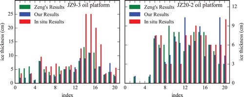
As shown in Table 3, retrieval results are similar to in situ observation data presented in Zeng et al. (2016) at the two oil platforms in the winter of 2009–2010. The bias at the JZ9-3 oil platform is much greater than that at the JZ20-2 oil platform (Figure 2). The root-mean-square error (RMSE) between our results and the in situ data are 6.42 and 2.26 cm at JZ9-3 and JZ20-2 oil platforms, respectively. The same values from the comparison between our results and Zeng’s are 2.16 and 2.57 cm. The greater bias at the location of the oil platform JZ9-3 is caused by the remarkable ice thickness (greater than 15 cm) during 2–4 February 2010. When data from these three days were excluded, the RMSE between our results and the in situ data and Zeng’s results decreased to 2.95 and 1.59 cm, respectively.

Figure 2. Retrieved ice thickness at the two oil platforms (JZ9-3 and JZ20-2) during the winter seasons of 2009–2010, based on Zeng’s result, our results (both are derived from MODIS data), and in situ observed ice thickness from Zeng et al. (2016). The index of the horizontal axis refers to time in Table 3.

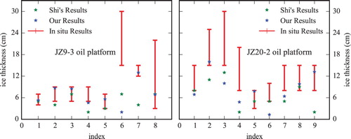
As shown in Table 4, in the winter of 2012–2013, our results are similar to the in situ observed data except for the results on 4 February 2013 at the JZ9-3 Oil Platform. The in situ ice thickness in Shi’s paper is presented as a range, not a specific value. Therefore, the RMSE cannot be calculated. On the other hand, only four values in Shi’s results are in the range of the in situ observed data (Figure 3). This suggests that the accuracy of our retrieval results is higher than that of Shi’s results. However, our results and Shi’s results at the JZ20-2 Oil Platform are not better than those at the JZ9-3 Oil Platform.

Figure 3. Retrieved ice thickness at the two oil platforms (JZ9-3 and JZ20-2) during the winter of 2012–2013, based on Shi’s result, our results (both are derived from MODIS data), and in situ observed ice thickness from Shi et al. (2016). Vertical bars represent the range of the in situ thickness measure.

In general, there are greater differences between estimated ice thicknesses from MODIS data and in situ observed data when ice thickness is greater than 15 cm. The ice thickness differences between our results and the in situ observed ice thickness or published results can be attributed to factors such as the ice movement during the time gap between MODIS acquisitions and in situ measurements. Spatial scale difference between in situ measurements and MODIS observations may also contribute to the differences. Moreover, errors may be caused by inaccuracy of IST estimation (RMSE approximately 1.2–1.3 K) and the use of the simplified sea ice surface heat balance equation (ice dynamics, including deformation and mechanical thickness growth due to rafting and ridging, are not considered in the equation). However, the retrieved ice thickness in this study was in reasonable agreement with the in situ observations and published results from the two offshore oil platforms over two winter seasons. This indicates that the ice thickness retrieved from MODIS data can be used for long-term analysis in the Bohai Sea.

5.2. Ice extent validation

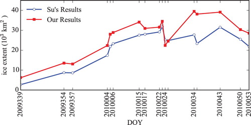
So far, only one study estimating ice extent in the Bohai Sea has been conducted. It was based on a threshold of band ratio from daytime MODIS data and results were available for the winter of 2009–2010 (Su, Wang, and Yang 2012). Comparison of SIE from our results against results from this study is presented in Figure 4. Although the same temporal trend is shown, our estimated SIE is usually larger. The difference may be due to the different methods used in obtaining the ice extent and the different resolution of data set. The RMSE of the difference between the two sets of results is 6440 km².

Figure 4. Retrieved ice extent of the Bohai Sea based on MODIS data and previously published results during the winter of 2009–2010.

6. Results

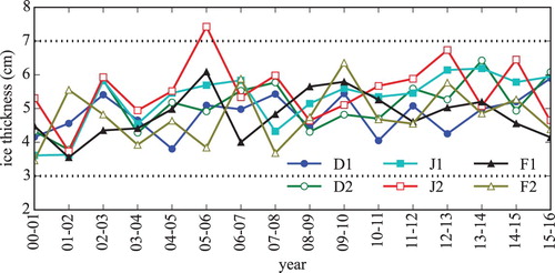
As shown in Table 1, there are 40–60 cloud-free MODIS images in most winter seasons during 2002–2016 except for the 13 images in the winter of 2000–2001 and 19 images in the winter of 2001–2002. The data are divided into six groups to mark the biweekly period during the three months of the investigation. The six groups are D1 (1–15 December), D2 (16–31 December), J1 (1–15 January), J2 (16– 31 January), F1 (1–15 February), and F2 (16– 28/29 February). In this study, ice thickness median is used in order to reduce the effect of anomalies on the statistics of the data.

6.1. The spatiotemporal patterns of SIT

As shown in Figure 5, the maximum ice thickness (mean value of all maximum ice thickness in each date group) in the Bohai Sea is usually found in J2. However, some exceptions occurred in the winter seasons of 2001–2002, 2006–2007, and 2009–2010 when ice thicknesses in F2 was significantly larger than in J2, and in the winter seasons of 2008–2009 and 2013–2014 when the maximum ice thickness occurred during other periods. The maximum ice thickness (around 5.58 cm) typically occurred in J2 as shown in Figure 5 and Table 4. This is the coldest period of the year with an average biweekly temperature of −5.4°C in contrast to −1.0°C in D1 and −1.9°C in F2. The median values of ice thickness ranged from 3 to 7 cm but it remained close to 5 cm during the most of the study period as shown in Figure 5. Annual variations of ice thickness fluctuate, but there is no identifiable increasing or decreasing trend between 2000 and 2016. No distinguished pattern can also be associated to any of the examined period. The mean values of ice thickness within each one of the six periods ranged between 4.7 and 5.6 cm. In D1 and F2, annual ice thickness was the thinnest. The Spearman correlation coefficients were calculated between mean ice thickness and average air temperature as −0.94 (P < .005), which suggests that air temperature is an important factor influencing the growth of ice thickness in the Bohai Sea.

Figure 5. Median values of SIT in the Bohai Sea for six periods from 2000 to 2016.

Table 6 includes the area of ice cover in square kilometers for ice with thickness ≥10 cm and <10 cm in the three bays connected to the Bohai Sea. The data showed that the thicker ice (≥10 cm thick) in Liaodong Bay had 1.2–1.6 times spatial coverage greater than the sum of coverage in Bohai Bay and Laizhou Bay. The area in Bohai Bay was 1.5 times larger than that in Laizhou Bay, which suggests that the thicker sea ice from 2000 to 2016 was mainly distributed in Liaodong Bay.

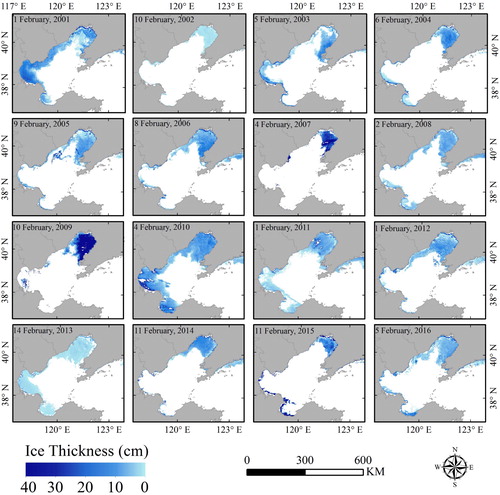
Ice thickness maps showing ice extent are presented in Figures 6 and 7. Results are consistent with findings from previous studies (Su and Wang 2012; Zeng et al. 2016). The figures show that SIT in Bohai Bay and Laizhou Bay was usually thinner than 5 cm and usually distributed in coastal regions. The area of mean ice thickness <10 cm in Liaodong Bay was also greater than that in Bohai Bay and Liaozhou Bay, and even larger than their sum. The area of mean SIT < 10 cm in Bohai Bay was at least twice as large as that in Laizhou Bay. Generally, the greatest sea ice condition was in Liaodong Bay (except for extreme cases in some years), then Bohai Bay, and the least was in Laizhou Bay. This is related to air temperature and geographic location. The mean air temperature from the AWS data in Liaodong Bay was −3.02°C in the 2000–2016 winter seasons, which was the lowest in the three bays (−1.83°C in Bohai Bay and −1.88°C in Laizhou Bay). Most of Liaodong Bay is north of 39°N, but Bohai Bay is located between 38°N and 39°N, and Laizhou Bay is south of 38°N.

Figure 6. SIT map of the Bohai Sea on the day when the maximum ice extent occurred in the six periods during the winter of 2009–2010.

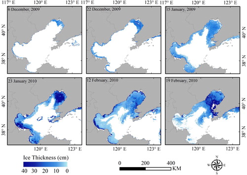
Figure 7. SIT map of the Bohai Sea on the day when the median ice extent occurred in each year during 2000–2016.

6.2. The spatiotemporal patterns of SIE

SIE in the Bohai Sea gradually increased from D1, reached its maximum value in F1, and then decreased as shown in Figure 8 and Table 5. The SIE in F1 was over four times larger than that in D1 when sea ice freeze-up began. The standard deviation values are relatively high, over 30% of the mean SIE for 2000–2016, and especially in F2 where it is approximately 60% of the mean SIE. In F1 in 2009–2010, the ice extent was the largest, nearly 40,000 km², which is double than that in F1 of 2001–2002, 2006–2007, 2013–2014, and 2014–2016. The winter of 2009–2010 was the coldest within the study period. The results show large annual variations in the mean SIE in the Bohai Sea with standard deviation (∼8000 km², over one-third of mean value) but with no temporal trend. Air temperature around the Bohai Sea gradually decreased from D1, and reached the mean minimum of −5.4°C in J2. Recall that the maximum SIE is observed in F1. There is no significant correlation between SIE and air temperature. However, the correlation coefficient between median SIE and negative accumulated temperature is −0.503 (P < .001) as shown in Figure 9.

Figure 8. SIE for six winter time periods during 2000–2016 in the Bohai Sea.

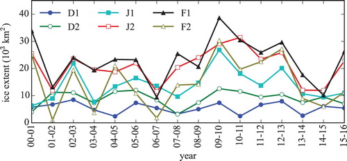
Figure 9. The evolution of negative accumulated temperature, SIE and SIT during 2000–2016.

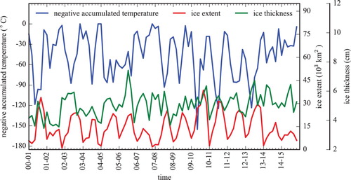
Table 5. Ice thickness, ice extent, and average temperature in the Bohai Sea during the in six winter periods, averaged over years 2000–2016.

		D1	D2	J1	J2	F1	F2
Mean value	Ice thickness (cm)	4.77 ± 0.52	5.04 ± 0.69	5.23 ± 0.80	5.58 ± 0.86	4.85 ± 0.66	4.80 ± 0.82
	Ice extent (km^2)	5491 ± 1969	9146 ± 2756	14,113 ± 5567	20,745 ± 6226	22,996 ± 8048	14,812 ± 8907
Range (median value)	Ice thickness (cm)	3.80–5.90 (4.98)	3.77–6.43 (5.06)	3.61–6.19 (5.28)	3.72–7.42 (5.42)	3.55–6.09 (4.72)	3.46–6.35 (4.71)
	Ice extent (km^2)	2396–8503 (5592)	3136–12,571 (9503)	6289–26,845 (13,488)	11,546–31,430 (22,378)	9404–38,635 (23,666)	1015–30,361 (14,058)
Mean air temperature (°C)		−1.0	−3.6	−5.3	−5.4	−3.9	−1.9

The negative accumulated temperature is the sum of the air temperature below −1.62°C (i.e. the freezing temperature of seawater with 30.0‰ salinity in the Bohai Sea) in each date group. The evolutions of the negative accumulated temperature, SIT, and SIE during each of the six periods for the entire study period (2000–2016) are shown in Figure 9. The correlation is lower than that between ice thickness and air temperature because SIE is influenced not only by air temperature but also by wind, ocean circulation, and snowfall. For example, snowfall increases the surface albedo (Grenfell and Perovich 2004), which leads to more solar radiation reflected back to the space. This results in colder ice surface and therefore accelerated ice growth and extent. In addition, snowfall increases in winter and can act as condensation nuclei for sea ice to formation.

As shown in Table 6 and Figure 10, the largest SIE occurred in Liaodong Bay, followed by Laizhou Bay, and then Bohai Bay. The area of Liaodong Bay is approximately 30,000 km², the area of Bohai Bay is approximately 15,900 km², and the area of Laizhou Bay is approximately 7000 km². In the past 16 years, the ratio of SIE to the total area of Liaodong Bay usually ranged approximately from 40% to 60%, and the maximum ratio was approximately 80% in the winter of 2009–2010 (Figure 10). The ratios of SIE in Bohai Bay and Laizhou Bay were similar and often lower than 40%, except during the winter seasons of 2009–2010 and 2010–2011, when the ratio was approximately 70%. According to Figures 6 and 7, sea ice in Liaodong Bay was the most expansive and consistent from year to year among the three bays. In Liaodong Bay, the frequency of sea ice decreased from the northeast coast to southwest open sea, and the sea ice edge was approximately 60–80 nautical miles away from the north coast. However, in Bohai Bay and Laizhou Bay, the frequency of sea ice decreased gradually from seashore to open sea, and the sea ice edge was approximately 20–30 and 15–25 nautical miles away from the northern coast, respectively.

Figure 10. Ratio of median SIE to area of each bay in F1 during 2000–2016.

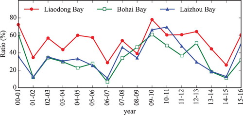
Table 6. Area of sea ice cover (km²) with mean ice thickness ≥10 cm and <10 cm in the three bays connected to the Bohai Sea, for each one of the six periods within the winter season, averaged over the study period (from 2000 to 2016).

	Mean ice thickness ≥ 10 cm			Mean ice thickness < 10 cm
	Liaodong Bay	Bohai Bay	Laizhou Bay	Liaodong Bay	Bohai Bay	Laizhou Bay
D1	435	165	101	2372	1691	674
D2	687	343	207	4224	2454	1057
J1	1229	540	339	6986	3388	1579
J2	1866	791	369	11,272	4639	2159
F1	1570	638	354	13,777	4763	2171
F2	1001	442	230	10,016	2643	994

6.3. The variations of air temperature around the Bohai Sea

Monthly air temperature from 21 AWS from 1951 to 2016 was obtained to explore the warming trend in the Bohai Sea. Surface air temperature trends in the northern polar area (NPA, the area north of 60°N) were obtained for comparison with the warming trend in the Bohai Sea. A simple moving average with a span of 5 years was employed to smoothen the data, reduce random fluctuations, and show the trend more clearly. Trends were achieved by linear regression using a least squares method. As indicated in Table 7, the trends in the three bays within the Bohai Sea are different, but all are positive, which indicates warming in recent decades for the Bohai Sea region. The trend in the Bohai Sea over the last 65 years (1951–2016) reveals an increase in temperature at a rate of 0.345°C per decade, but this rate has been reduced to 0.277°C per decade since 1979. A similar result is found for both Liaodong Bay and Laizhou Bay. The season with the highest increase is winter, followed by spring and autumn, while summer demonstrates the smallest rate of temperature warming. However, the warming rate in the Bohai Sea and the three bays became inconsistent since 1979. This may be related to geographic location, industrial development, and regional and global climate changes. Trends in Bohai Bay, which is adjacent to the Jing-Jin-Ji Area in the third economic circle, are the largest during 1979–2016. The economic growth, triggered mainly by industrial development, around the Bohai Sea may have contributed to the warming.

Table 7. Trends of air temperature increases (°C per decade) in the Bohai Sea, the three bays, and the NPA.

	1951–2016					1979–2016
	Winter	Spring	Summer	Autumn	annual	Winter	Spring	Summer	Autumn	annual
Bohai Sea	0.497	0.403	0.189	0.314	0.345	0.271*	0.324	0.209	0.341	0.277
Liaodong Bay	0.541	0.400	0.155	0.345	0.354	0.279	0.308	0.177	0.343	0.267
Bohai Bay	0.394	0.319	0.118	0.232	0.262	0.403	0.322	0.179	0.400	0.317
Laizhou Bay	0.382	0.351	0.201	0.243	0.287	0.192*	0.292	0.207	0.287	0.237
NPA	0.381	0.467	0.234	0.361	0.364	0.648	0.707	0.437	0.754	0.639

Note: Winter refers to December, January, and February; spring refers to March, April, and May; summer refers to June, July, and August; and autumn refers to September, October, and November.

*P < .05, for other data P < .001, P values of the trend values in NPA were not provided in Bekryaev’s paper but it has been stated that the trends are statistically significant.

For 1951–2016, the trends in NPA are consistent with those in the Bohai Sea and the three bays, and the differences are small. However, for 1979–2016, the trends in NPA are greater than those in the Bohai Sea and the three bays, and the increasing warming rates are often twice as large as those in the Bohai region. Variations in SIE and SIT in the Bohai Sea for 2000–2016 fluctuate, yet with no observed trend. SIE does not decrease with warming, and SIT is responsive to the temperature but not a confirming longer-term trend.

7. Discussion

Ice thickness growth is affected by many factors, such as salinity, wind, air temperature, and water temperature. SIT estimation using the surface heat balance equation is sensitive to temperature and wind speed, especially the difference between air temperature and ice temperature (Zeng et al. 2016). In this study, the errors in estimated SIT may be caused by inaccuracies in estimated air temperature and wind speed, both obtained from ERA-Interim reanalysis data. There are differences between the reanalysis data and AWS observation data despite their general agreement, which can result in uncertainties in SIT estimation. There are significant spatial variations in salinity in the Bohai Sea, ranging between 26‰ and 33‰, which suggests that freezing temperatures vary from −1.40°C to −1.78°C. However, in this study, a salinity of 30‰ was employed in the SIT calculation, which indicates that the freezing temperature was approximately −1.62°C. This can be another source of error in the calculations of the SIT. The accuracy of IST estimation using the split-window technique is approximately 1.2–1.3 K, which also leads to errors in the estimated SIT. The IST, also called the skin temperature, is retrieved from TIR radiation emitted only from the top few millimeters of the ice cover. This may constitute another source of error. The ice thickness differences between our results and in situ observations and published results can be attributed to ice movement during the time delay between MODIS acquisitions and the in situ measurements, that is in addition to the spatial scale difference between in situ measurements and MODIS data. In the heat balance equation of the sea ice surface, ice dynamics are not considered, which likely induces unexpected errors. However, the retrieved ice thickness in this study was in reasonable agreement with in situ observations and published results from two offshore oil platforms in two winter seasons, which indicates that the ice thickness retrieved from MODIS data can be used for long-term analysis in the Bohai Sea.

SIE is obtained from SIT when it is greater than 0. In this study, if the IST of a pixel is lower than −1.62°C, the retrieved SIT of the pixel may be larger than 0, and then the pixel would be included in the SIE calculations. The difference between our results and the results published in Su and Wang (2012) can be attributed to the different methods and different resolution of data set for obtaining SIE. In general, results show that the ice extent retrieved from MODIS data is reliable.

The air temperature in the Bohai Sea and the three bays connected to it shows increasing trends during 1951–2016 and 1979–2016, but the rate of increase is much less than that in the NPA. This suggests that the mid-latitude monsoon climate zone is warming at a rate less than the NPA. Observation data from more sites should be collected for further analysis of warming in the mid-latitude monsoon climate zone.

8. Conclusion

In this study, SIT in the Bohai Sea from 2000 to 2016 was achieved using MODIS L1B data and ECMWF reanalysis data based on a split-window technique and the surface heat balance equation. The results show that the retrieved SIT and SIE are in good agreement with in situ observations and published results and can be used for long-term analysis. To explore the temporal variation of sea ice, we divided the results into six date intervals (on a biweekly basis). The period with the greatest ice thickness was J2 (second half of January), while the period with the greatest ice extent was F1 (first half of February). The mean SIT and SIE from 2000 to 2016 were 5.58 ± 0.86 cm and 22,996 ± 8048 km², respectively. The variation in mean ice thickness was slight, within the range of 3–7 cm between the different periods. However, SIE varied to a larger degree. The SIE maximum during F1 was approximately 38,000 km² in 2010. Prior to 2010, the ice extent was generally in the range of 2000–3000 km², except in 2007 when it was approximately 9400 km². Since 2010, SIE has gradually decreased except in 2012 when it was 13,000 km².

Among the three bays, sea ice in Liaodong Bay is the most extensive and consistent from year to year. It extended from the northeast coast to the southwest open sea, and the sea ice edge was approximately 60–80 nautical miles away from the north coast. However, in Bohai Bay and Laizhou Bay, sea ice decreased gradually from seashore to open sea, and the sea ice edge was approximately 20–30 and 15–25 nautical miles away from the respective north coasts.

The air temperature warming rate has increased in the Bohai Sea over the last 65 years (1951–2016) at 0.345°C per decade, but has decreased to 0.277°C per decade since 1979, which is lower than the rate in NPA. In particular, the increasing warming rate in NPA is slightly more than twice the rate in the Bohai Sea since 1979. However, given the existing warming trend in the Bohai Sea, no parallel trend in SIT or SIE is found during the study period (from 2000 to 2016). The ice conditions are related to local climate, especially severe weather events. This also implies that sea ice in the Bohai Sea, as a natural hazard causing economic damage, should be subject to better monitoring and forecasting.

Acknowledgements

The authors are grateful to NASA’s Level-1 and Atmosphere Archive & Distribution System (LAADS) Distributed Active Archive Center (DAAC) for providing daily MODIS imagery of the Bohai Sea, the European Centre for Medium-Range Weather Forecasts (ECMWF) for providing ERA-Interim reanalysis data including wind speed and air temperature, and the Climatic Data Center of the National Meteorological Information Center at the China Meteorological Administration for providing daily air temperature from 21 automatic weather stations around the Bohai Sea. Last but not least, the authors wish to thank the anonymous reviewers who did a thorough critical review of the manuscript and provided valuable suggestions to improve it.

Disclosure statement

No potential conflict of interest was reported by the authors.

Additional information

Funding

This work was supported by the Chinese Arctic and Antarctic Administration, National Natural Science Foundation of China (Grant Nos. 41676176, 41676182 and 41428603), and Chinese Polar Environment Comprehensive Investigation and Assessment Program.

References

- Adams, S., S. Willmes, D. Schröder, and G. Heinemann. 2013. “Improvement and Sensitivity Analysis of Thermal Thin-Ice Thickness Retrievals.” IEEE Transactions on Geoscience and Remote Sensing 51: 3306–3318. doi: 10.1109/TGRS.2012.2219539
- Bai, S., Q. Liu, H. Li, and H. Wu. 1999. “Sea Ice in the Bohai Sea of China.” [In Chinese] Marine Forecasts 16: 1–8.
- Bai, S., and H. Wu. 1998. “Numerical Sea Ice Forecast for the Bohai Sea.” [In Chinese] Acta Meteorologica Sinica 56: 139–153.
- Dieckmann, G. S., and H. H. Hellmer. 2010. “The Importance of Sea Ice: An Overview.” In Sea Ice, 2nd ed., edited by David N. Thomas and Gerhard S. Dieckmann, 1–22. Oxford, UK: Wiley-Blackwell.
- Giles, K. A., S. W. Laxon, and A. L. Ridout. 2008. “Circumpolar Thinning of Arctic Sea Ice Following the 2007 Record Ice Extent Minimum.” Geophysical Research Letters 35: L22502. doi:10.1029/2008GL035710.
- Grenfell, T. C., and D. K. Perovich. 2004. “Seasonal and Spatial Evolution of Albedo in a Snow-Ice-Land-Ocean Environment.” Journal of Geophysical Research 109: C01001. doi:10.1029/2003JC001866.
- Guo, Q., Y. Chen, J. Li, L. Ri, and X. Shi. 2006. “The Progress of Remote Sensing on Sea Ice Research in China.” [In Chinese] Marine Forecasts 23: 95–103.
- Hall, D. K., J. R. Key, K. A. Casey, G. A. Riggs, and D. J. Cavalieri. 2004. “Sea Ice Surface Temperature Product From MODIS.” IEEE Transactions on Geoscience and Remote Sensing 42: 1076–1087. doi: 10.1109/TGRS.2004.825587
- Huntemann, M., G. Heygster, L. Kaleschke, T. Krumpen, M. Mäkynen, and M. Drusch. 2014. “Empirical Sea Ice Thickness Retrieval During the Freeze-up Period From SMOS High Incident Angle Observations.” The Cryosphere 8: 439–451. doi: 10.5194/tc-8-439-2014
- Kaleschke, L., X. Tian-Kunze, N. Maaß, A. Beitsch, A. Wernecke, M. Miernecki, G. Müller, et al. 2016. “SMOS Sea Ice Product: Operational Application and Validation in the Barents Sea Marginal Ice Zone.” Remote Sensing of Environment 180: 264–273. http://doi.org/10.1016/j.rse.2016.03.009.
- Karvonen, J., L. Shi, B. Cheng, M. Similä, M. Mäkynen, and T. Vihma. 2017. “Bohai Sea Ice Parameter Estimation Based on Thermodynamic Ice Model and Earth Observation Data.” Remote Sensing 9: 234. doi: 10.3390/rs9030234
- Kim, J., D. Kim, and B. J. Hwang. 2012. “Characterization of Arctic Sea Ice Thickness Using High-Resolution Spaceborne Polarimetric SAR Data.” IEEE Transactions on Geoscience and Remote Sensing 50: 13–22. doi: 10.1109/TGRS.2011.2160070
- Kurtz, N. T., N. Galin, and M. Studinger. 2014. “An Improved CryoSat-2 Sea Ice Freeboard Retrieval Algorithm Through the Use of Waveform Fitting.” The Cryosphere 8: 1217–1237. doi: 10.5194/tc-8-1217-2014
- Laxon, S. W., K. A. Giles, A. L. Ridout, D. J. Wingham, R. Willatt, R. Cullen, R. Kwok, A. Schweiger, J. Zhang, and C. Haas. 2013. “CryoSat-2 Estimates of Arctic Sea Ice Thickness and Volume.” Geophysical Research Letters 40: 732–737. doi: 10.1002/grl.50193
- Laxon, S., N. Peacock, and D. Smith. 2003. “High Interannual Variability of Sea Ice Thickness in the Arctic Region.” Nature 425: 947–950. doi: 10.1038/nature02050
- Li, Z., and Y. Wang. 2001. “Statistical Ice Conditions of Bohai Sea.” Paper presented at the Proceedings of the International Conference on Offshore Mechanics and Arctic Engineering, Rio de Janeiro, Brazil.
- Liu, C., J. Chao, W. Gu, Y. Xu, and F. Xie. 2015. “Estimation of Sea Ice Thickness in the Bohai Sea Using a Combination of VIS/NIR and SAR Images.” GIScience & Remote Sensing 52: 115–130. doi: 10.1080/15481603.2015.1007777
- Liu, J., R. Huang, Z. Jin, K. Wu, and C. Sun. 2000. “Bohai Sea Ice Monitoring Using Satellite Images.” Journal of Cold Regions Engineering 14: 93–100. doi: 10.1061/(ASCE)0887-381X(2000)14:2(93)
- Liu, W., H. Sheng, and X. Zhang. 2016. “Sea Ice Thickness Estimation in the Bohai Sea Using Geostationary Ocean Color Imager Data.” Acta Oceanologica Sinica 35: 105–112. doi: 10.1007/s13131-016-0910-1
- Luo, Y., H. Wu, Y. Zhang, C. Sun, and Y. Liu. 2004. “Application of the HY-1 Satellite to Sea Ice Monitoring and Forecasting.” Acta Oceanologica Sinica 23: 251–266.
- Martin, S., R. Drucker, R. Kwok, and B. Holt. 2004. “Estimation of the Thin ice Thickness and Heat Flux for the Chukchi Sea Alaskan Coast Polynya From Special Sensor Microwave/Imager Data, 1990–2001.” Journal of Geophysical Research: Oceans 109: C10012. doi:10.1029/2004JC002428.
- Maykut, G. A. 1982. “Large-Scale Heat Exchange and Ice Production in the Central Arctic.” Journal of Geophysical Research 87: 7971–7984. doi: 10.1029/JC087iC10p07971
- Nakamura, K., H. Wakabayashi, K. Naoki, F. Nishio, T. Moriyama, and S. Uratsuka. 2005. “Observation of Sea-Ice Thickness in the Sea of Okhotsk by Using Dual-Frequency and Fully Polarimetric Airborne SAR (Pi-SAR) Data.” IEEE Transactions on Geoscience and Remote Sensing 43: 2460–2469. doi: 10.1109/TGRS.2005.853928
- Nakawo, M., and N. K. Sinha. 1981. “Growth Rate and Salinity Profile of First-Year Sea Ice in the High Arctic.” Journal of Glaciology 27: 315–330. doi: 10.1017/S0022143000015409
- Ning, L., F. Xie, W. Gu, Y. Xu, S. Huang, S. Yuan, T. Cui, and J. Levy. 2009. “Using Remote Sensing to Estimate Sea Ice Thickness in the Bohai Sea, China Based on Ice Type.” International Journal of Remote Sensing 30: 4539–4552. doi: 10.1080/01431160802592542
- Riggs, G. A., D. K. Hall, and V. V. Salomonson. 2006. “MODIS Sea Ice Products User Guide to Collection 5.” National Snow and Ice Data Center, University of Colorado, Boulder, CO, USA.
- Shi, L., T. Zeng, M. Makynen, and B. Cheng. 2016. “Sea Ice Thickness Retrieval with Modis Thermal Infrared Data over the Liaodong Bay During Winter 2012–2013”. Paper presented at the IGARSS 2016–2016 IEEE International Geoscience and Remote Sensing Symposium.
- Song, Q., J. Zhang, T. Cui, and Y. Bao. 2013. “Retrieval of Sea Surface Salinity with MERIS and MODIS Data in the Bohai Sea.” Remote Sensing of Environment 136: 117–125. doi: 10.1016/j.rse.2013.05.017
- Su, H., and Y. Wang. 2012. “Using MODIS Data to Estimate Sea Ice Thickness in the Bohai Sea (China) in the 2009-2010 Winter.” Journal of Geophysical Research 117: 995–1000.
- Su, H., Y. Wang, J. Xiao, and X. Yan. 2015. “Classification of MODIS Images Combining Surface Temperature and Texture Features Using the Support Vector Machine Method for Estimation of the Extent of Sea Ice in the Frozen Bohai Bay, China.” International Journal of Remote Sensing 36: 2734–2750. doi: 10.1080/01431161.2015.1041619
- Su, H., Y. Wang, and J. Yang. 2012. “Monitoring the Spatiotemporal Evolution of Sea Ice in the Bohai Sea in the 2009–2010 Winter Combining MODIS and Meteorological Data.” Estuaries and Coasts 35: 281–291. doi: 10.1007/s12237-011-9425-3
- Tian-Kunze, X., L. Kaleschke, N. Maaß, M. Mäkynen, N. Serra, M. Drusch, and T. Krumpen. 2014. “SMOS-derived Thin sea ice Thickness: Algorithm Baseline, Product Specifications and Initial Verification.” The Cryosphere 8: 997–1018. doi: 10.5194/tc-8-997-2014
- Wu, D., X. Wan, X. Bao, M. Lin, and L. Jian. 2004. “Comparison of Summer Thermohaline Field and Circulation Structure of the Bohai Sea Between 1958 and 2000.” Chinese Science Bulletin 49: 363–369. doi: 10.1007/BF02900319
- Yang, G. 2000. “Bohai Sea Ice Conditions.” Journal of Cold Regions Engineering 14: 54–67. doi: 10.1061/(ASCE)0887-381X(2000)14:2(54)
- Yu, Y., and R. W. Lindsay. 2003. “Comparison of Thin Ice Thickness Distributions Derived From RADARSAT Geophysical Processor System and Advanced Very High Resolution Radiometer Data Sets.” Journal of Geophysical Research 108: 226–231.
- Yu, Y., and D. A. Rothrock. 1996. “Thin Ice Thickness From Satellite Thermal Imagery.” Journal of Geophysical Research: Oceans 101: 25753–25766. doi: 10.1029/96JC02242
- Zeng, T., L. Shi, M. Makynen, B. Cheng, J. Zou, and Z. Zhang. 2016. “Sea Ice Thickness Analyses for the Bohai Sea Using MODIS Thermal Infrared Imagery.” Acta Oceanologica Sinica 35: 96–104. doi: 10.1007/s13131-016-0908-8
- Zwally, H. J., D. Yi, R. Kwok, and Y. Zhao. 2008. “ICESat Measurements of Sea Ice Freeboard and Estimates of Sea Ice Thickness in the Weddell Sea.” Journal of Geophysical Research 113: 228–236. doi: 10.1029/2007JC004284