A virtual globe-based time-critical adaptive visualization method for 3D city models

ABSTRACT

3D city models, which are important items of content on the virtual globe, are characterized by complicated structures and large amounts of data. These factors make the visualization of 3D city models highly dependent upon the performance of computer hardware. Thus, achieving the efficient rendering of 3D city models using different hardware performance levels represents one of the key problems currently facing researchers. This paper proposes a time-critical adaptive visualization method that first estimates the possible rendering time for each model according to the data structure of the model in addition to the CPU/GPU performance of the computer. It then dynamically adjusts the rendering level for each model based on the results of an estimation of the rendering time to ensure that the final scene can be completed within a given time. To verify the effectiveness and flexibility of this method, it is applied using different computers. The results show that the adaptive visualization method presented in this paper not only can adapt to computers with different levels of performances but also demonstrates an obvious improvement in the time estimation precision, visual effects, and optimization speed relative to existing adaptive visualization methods.

KEYWORDS:

• Virtual globe
• 3D city model
• adaptive visualization

1. Introduction

With the continuous development of approaches for city modeling and the increase in the requirements for 3D scene fidelity, 3D city models are characterized by a complicated structure, intensive distribution, and large amounts of data (Chen et al. 2014; Ellul and Altenbuchner 2014; Zhang et al. 2014). All of these factors make the visualization of 3D city models highly dependent on the performance of the computer hardware employed. Meanwhile, the different capabilities of computer hardware are diverging. Due to the huge performance gap between different types of computer hardware, the use of individual visualization strategies to render 3D city models is difficult given the varying needs of different terminal users. Therefore, the automatic optimization of 3D city scenes according to the level of performance of the computer while simultaneously efficiently rendering the scenes using different types of hardware (i.e. so-called adaptive visualization) has become a salient issue in research related to geographical information visualization.

Adaptive visualization can essentially be considered as a means to achieve an optimal rendering of a 3D scene within a limited time frame (Funkhouser and Séquin 1993). To resolve the problems therein, at least two aspects must be addressed: how to estimate the rendering time and how to optimize the scene. To estimate the rendering time, existing methods mainly estimate the rendering time for an object by using geometric information, such as the number of vertices or triangles (Dong et al. 2015). For 3D city models, especially modern building models, the texture is often more complex than the geometry (Zhang, Zhu, and Hu 2007). It is difficult to guarantee the estimation accuracy based only on geometric information. Furthermore, multi-threaded data loading is key to the visualization of massive amounts of 3D city model data. But frequent data loading and unloading processes have a huge impact on the rendering time, this has not been considered by existing methods. To optimize a scene, existing methods achieve their goals by dynamically adjusting the level of detail (LOD) for each rendering object, which cannot guarantee the convergence speed of the algorithm when applied to a large scene (e.g. when there are more than 1000 3D city models) and eventually affects the rendering efficiency.

Given the characteristics of 3D city models, this paper proposes a new adaptive visualization method, which is mainly divided into two parts. First, to improve the accuracy of the time estimate, this paper improves the existing rendering time estimation methods. This new method not only considers the characteristics of the data structure of 3D city models but also reduces the influence of multi-threaded data loading on the estimation accuracy as much as possible. Second, to improve the scene optimization speed, a tiled quadtree organization of the virtual globe is combined with a scene optimization algorithm, by using tiles instead of a single model to participate in the iterative calculation, the optimized convergence time is effectively reduced. At the same time, the new optimization algorithm takes the overall features of a scene into consideration and, thus, a better visual effect can be attained. The effectiveness of the method is verified by means of contrast experiments.

2. Related work

According to the characteristics of related technologies, adaptive visualization can be mainly divided into three categories: adaptive visualization based on multiple data sets, adaptive visualization based on LOD control, and adaptive visualization based on remote rendering (Koskela and Vatjus-Anttila 2015).

Compared with the other two methods, adaptive visualization based on multiple data sets is the simplest to achieve. It adapts to different terminals by using different levels of accuracy data sets. For example, by building multiple data sets in advance, the terminal can choose the appropriate data set according to the performance of the terminal (Krebs, Marsic, and Dorohonceanu 2002). However, this method ignores the influence of the complexity of a 3D scene on the visualization process, especially that of 3D city models, which is characterized by changes in the intensity and complexity of the model according to the specific scene. Thus, setting the accuracy of data for every scene based only on the hardware performance cannot fundamentally satisfy the requirements for adaptively visualizing 3D city models.

Adaptive visualization based on LOD control is an extension of visualization based on multiple data sets. As a result of using LOD dynamic control, its application is more flexible. Funkhouser and Séquin (1993) first proposed a method based on the visual gain and time cost of a discrete LOD model; when the rendering time is less than the specified time, an LOD is chosen for each of the visible objects such that those objects have the maximum visual effect. Since then, many experts and scholars (Zach, Mantler, and Karner 2002; Hernández and Beneš 2005; Zhang, Zhu, and Hu 2007; Yu, Liang, and Chen 2008; Sunshine-Hill 2013; Dong et al. 2015) have improved upon this approach and proposed more precise methods for calculating the visual gain and time cost in their respective applications. However, the problem of the optimal selection of the LOD can essentially be regarded as an instance of the multiple-choice knapsack problem (MCKP), and the complexity of solving the MCKP is so great that it cannot be performed in real time. Therefore, Funkhouser and Séquin (1993) used a simple greedy approximation algorithm in which items are placed into the knapsack in a decreasing order of value. However, their results are only half as good as the optimum solution, and there is a risk that low-value rendering objects may not be displayed. Meanwhile, it is difficult to ensure an acceptable level of efficiency when the number of rendering objects is large due to the need to sort the rendering objects according to their values.

To counteract the limitations of the discrete LOD model, Gobbetti et al. (2012), Lavoué, Chevalier, and Dupont (2013), and Lee, Lavoué, and Dupont (2012) researched the control of a continuous LOD model, since a continuous LOD model can be organized into the form of a workflow, and the control of the said flow is more flexible relative to the discrete LOD model. As such, it can improve upon the convergence speed of the optimization by simplifying the calculations for the visual gain and time cost. However, a continuous LOD is mainly oriented toward a model with a complex geometrical surface. For 3D city models, and especially for modern building models that mainly consist of a large amount of simple textural geometries, it is difficult to build a continuous LOD directly.

Unlike previous methods, visualization based on remote rendering (Preda et al. 2008; Nijdam et al. 2010; Doellner, Hagedorn, and Klimke 2012) fully assigns high-complexity computational tasks to the server, and the terminal is only responsible for rendering the final results (i.e. the image). Thus, it fundamentally eliminates the influence that heterogeneous devices have on the rendering of 3D graphics. However, this approach requires high-frequency real-time communication between the client and the server, and thus, network delays will prevent the user from obtaining a quick response from the server, which will affect the user’s experience. To implement the visualization of a 3D scene according to the network bandwidth, Nijdam et al. (2010) determined the optimal size for an image based on the current network bandwidth and determined the image compression mode according to the terminal’s ability to render the images and decompress the data. However, this method was overly dependent on the server and did not make full use of the existing hardware resources of the terminal. With the ongoing development of computer technology, the performance of terminal hardware is also constantly improving. Therefore, this type of visualization technology whereby all processing is performed by the server to avoid the influences of differences in the terminal hardware performance is not the best solution.

To summarize, existing adaptive visualization methods mainly ensure the stability of the rendering efficiency by optimizing the LOD control strategy and then satisfy the need to adapt to different levels of terminal performance. However, due to the characteristics of 3D city models (i.e. their large amounts of data, uneven distributions, and different complexities), such precision and efficiency cannot be guaranteed when directly applying existing adaptive visualization methods based on LOD control to 3D city models. Therefore, this paper proposes a new adaptive visualization method for 3D city models.

The remainder of this paper is organized as follows. Section 3 provides the methodology with two subsections. Section 3.1 describes how to estimate the possible rendering time for each model according to the data structure of the 3D city model, and Section 3.2 describes how to dynamically adjust the LOD for each model based on the results of the estimation of the rendering time to ensure that the final scene can be completed within a given time. Section 4 verifies the validity of this proposed method according to three aspects. Section 5 concludes the study and discusses future work.

3. Methodology

As mentioned above, the main aspects of adaptive visualization addressed in this paper are (1) rendering time estimation and (2) scene optimization.

3.1. Rendering time estimation

Although the actual rendering time of an object is influenced by a variety of factors, it can still be roughly estimated by making simplified assumptions. This estimation method is more efficient and can be adapted to most systems.

Because the rendering time is closely related to the data structure and the rendering method applied to the object being rendered, the time estimation methods proposed for different fields of application (Funkhouser and Séquin 1993; Wimmer and Wonka 2003; Lakhia 2004; Hernández and Beneš 2005; Zhang, Zhu, and Hu 2007; Dong et al. 2015) are often different. However, case studies have shown that the approach proposed by Wimmer and Wonka (2003) is a more comprehensive consideration of the influences that graphics rendering processes have on the rendering time and, thus, their method is more universal.

Wimmer and Wonka (2003) proposed subdividing the rendering process into two parallel parts: CPU rendering and GPU rendering. The CPU is responsible for culling a scene and switching the rendering state and the transmission of the vertex arrays. The GPU handles the conversion of the coordinates of the vertexes and the raster of the primitives. The final rendering time is determined by the slowest part. They consequently proposed a time estimation model as follows:where RT_system is the time required to perform a system task and can be viewed as a constant, RT_cpu is the rendering time of the CPU, and RT_gpu is the rendering time of the GPU. The time estimation model for the GPU is as follows:(1) where #tv is the number of vertices to be converted, #pix is the number of pixels, and c1, c2 … cn are constants related to the specific hardware performance that can be obtained by a regression analysis of the sample points.

Wimmer and Wonka (2003) proposed that the rendering time of the CPU is related to the specific scene organization and rendering process; thus, they did not attempt to produce a detailed time estimation model for the CPU, which we have succeeded in adding within the present study. To better illustrate the design of the time estimation model for the CPU, the basic rendering process for the 3D city model is first introduced as shown in Figure 1. The dashed box of CPU (render thread) indicates that the process is executed within the CPU rendering thread, the dashed box of CPU (load thread) indicates that the process is executed within the CPU loading thread, and the dashed box of GPU indicates that the process is executed within the GPU.

Figure 1. Basic rendering process of the 3D city model.

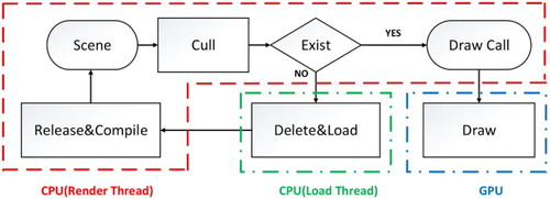
Here, the rendering thread is mainly responsible for the culling of a scene (Cull) and the sending of drawing calls (Draw Call), while the loading thread is responsible for loading the model data into the memory (Load). Without considering the immediate mode in OpenGL, the model data must be compiled into an OpenGL object (Compile) before the Draw process.

This manner of loading the data by opening the thread can reduce the influence that a complex data parsing process has on the rendering thread, which is key to achieving the visualization of a massive 3D city model. However, this multi-threaded method will increasingly complicate the estimation of the rendering time such that the estimation accuracy will be difficult to guarantee. To reduce the influence that multi-threaded data loading has on the estimation of the rendering time, the present study considers the following measures.

1. Reducing the conflicts in the occupation of system resources between the rendering thread and loading thread. The number of loading threads that can be opened at the same time is fixed, so any new loading request must wait in a queue. The priority of a loading thread is reduced to a minimum, and the loading thread does not run on the same CPU core as the rendering thread.

2. Controlling the transmission from the loading thread to the rendering thread to limit the time that an OpenGL object in each frame requires for Release & Compile.

3. Preventing memory jitter. Using the memory pool, the data are unloaded from a queue item-by-item during idle time, thereby avoiding bulk unloading.

The averaging of this approach can eliminate the influence that multi-threaded data loading has on the rendering time for each frame such that the affected values can be fixed for estimation.

According to Figure 1, after fixing the influence that multi-threaded data loading has on the rendering time, the rendering time of the CPU can be determined as the sum of the scene culling time (RT_cull) and the drawing call time (RT_drawcall):The main purpose of Cull is to perform a visibility analysis on the rendering objects (i.e. culling the smallest bounding box of the rendering objects according to the view frustum). Because the computing time required for the process is almost fixed, it can be represented linearly by the number of bounding boxes. At the same time, given that the model matrix is generally used to achieve a transformation from the local coordinates to the global coordinates of the objects being rendered, the view frustum needs to be updated when encountering an object that contains a model matrix, thereby making this process more time-consuming. Therefore,where #matrix is the number of model matrices and #boundingbox is the number of bounding boxes.

The entire process of setting the rendering state and the vertex array of a rendering object is called ‘draw call.’ When using the vertex buffer object or a display list as the rendering mode, the vertex array is loaded into the GPU during the compile process and, thus, the time required for draw call is mainly consumed by setting the rendering state. For a 3D city model, the rendering state is dominated by the material texture and, thus, the consumption can be linearly represented by the number of textures (#texture):In addition, it is difficult to precisely calculate the number of pixels in real time. Therefore, the number of pixels (#pix) in Equation (1) is replaced by the projected area of the bounding box of the rendering object on the screen.

3.2. Scene optimization

3.2.1. Overall concept

As mentioned above, the MCKP problem is represented by trying to achieve the optimal rendering of a scene within a limited amount of time. Considering that it is difficult to solve the MCKP problem in real time, existing methods attempt to approximate the optimal solution iteratively. At present, scene optimization for the discrete LOD model commonly adopts a greedy algorithm, which traverses the objects in order of importance (Funkhouser and Séquin 1993; Zhang, Zhu, and Hu 2007; Sunshine-Hill 2013; Dong et al. 2015). The basic concept of the algorithm is as follows: if the rendering time is greater than the time that is available, the objects are traversed in order of importance from small to large while reducing the level one-by-one; if the rendering time is less than the available time, the objects are traversed in order of importance from large to small while increasing the rendering level one-by-one. This approach is simple to implement, but it is likely to result in a large number of unimportant objects being lost (Hernández and Beneš 2005). Furthermore, because each model in the scene must be sorted, the convergence speed of this algorithm is poor when the number of objects is large or when the scene is scanned quickly (Lakhia 2004).

In this paper, a new scene optimization algorithm is proposed, the basic concept of which is as follows. During the data processing stage, the discrete 3D city model is reorganized into a tiled quadtree of the virtual globe in which the tiles are used to replace the models for sorting purposes. This achieves the purpose of speeding up the convergence. When the algorithm is running, the maximum number of 3D city models that can be rendered within the available rendering time is determined first (i.e. assuming that each model is rendered at the lowest level). Then, the LOD of each model is increased according to its priority. If an increase in the LOD will result in a longer rendering time than is available, the least-important rendering object will be removed, or the LOD will be lowered to decrease the rendering time to reach the target time.

3.2.2. Data preprocessing

3D city models are characterized by a dense deployment and a large amount of data. If each model is processed separately, the computing time of the optimal algorithm will increase, and the efficiency of the rendering will decrease. Therefore, we organize the 3D city models into a top-down tiled quadtree (tile pyramid) based on the concept of a discrete global grid on a virtual globe (Figure 2).

Figure 2. Data organization of the 3D city models.

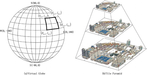
In the proposed data structure, the LodModel is used to represent the building units. Each LodModel can be included within the Tile of different levels. The quantity of the LodModel in the superior Tile is diluted by that of the LodModel in the subordinate Tile. The main LodModels should be preserved and well distributed during the dilution process. On each Tile, the LodModels are sorted according to its importance as previously assessed by semantics and the model size.

In practice, the Tiles are traversed from top to bottom and subdivided subordinate Tiles based on the distance from the viewpoint to the Tile center. Note that Tile and LodModel are only used as indices. The geometry and texture data for rendering are included in the Model (Child node of LodModel). LodModel determines which Model to load or draw based on the distance from the viewpoint to the LodModel center.

3.2.3. Cull LodModel

In order to determine which LodModels can be rendered within the given time, the tiled quadtree is traversed, and the Tiles are collected, after which the LodModels are extracted from the collected Tiles. The rendering time of each LodModel is estimated during the extraction. Once the total time of the rendering is estimated to be greater than the given time, the extraction is stopped; the detail algorithm is shown in Algorithm 1.

Algorithm 1:

Input: given time for rendering (TargetRenderTime), root of the tiled quadtree (Root), current view point (ViewPoint)

Output: set of LodModel (LodModelGroup), residual available CPU time (CPUAvailable), residual available GPU time (GPUAvailable)

• Step 1. Traverse the tiled quadtree from the Root and collect the Tiles in the view frustum;

• Step 2. Sort the Tiles according to their distance to ViewPoint and record the time needed to complete Step 1 and Step 2 (QuadTileTime);

•  Step 3: set CPUAvailable = TargetRenderTime-QuadTileTime and GPUAvailable = TargetRenderTime;

• Step 4:

•   For each Tile

•      For each LodModel

•        Get the lowest-level Model from LodModel;

•        If Model does not exist or is not in the view frustum

•          Continue;

•        Determine the statistics of the number of textures, vertices, matrices, and bounding boxes;

•        Calculate the number of pixels;

•        Estimate the time spent by the CPU and GPU (CPUTaken and GPUTaken, respectively) based on Section 3.1;

•        If CPUTaken > CPUAvailable or if GPUTaken > GPUAvailable

•          Go to Step 5;

•        Else

•          Insert LodModel into LodModelGroup;

•        CPUAvailable = CPUAvailable-CPUtaken and GPUAvailable = GPUAvailable-GPUTaken

•      End for

•   End for

• Step 5: CPUAvailable = CPUAvailable – the time spent by Step 4;

•    End algorithm;

Since the LodModels in the Tiles have been sorted according to their semantics and size, LodModels in LodModelGroup will be automatically sorted by their importance (i.e. semantics, size, and distance) by Algorithm 1.

3.2.4. LOD selection

After extracting the LodModels from the Tiles by Algorithm 1, the next step is to adjust the rendering level of LodModels so that the visual effect is as good as possible. If the increase in the LOD results in a longer rendering time than is available (GPUAvailable or CPUAvailable), the least-important rendering object will be removed, or the rendering level will be lowered to reduce the rendering time. The detailed algorithm is shown in Algorithm 2.

Algorithm 2:

Input: The set of LodModel (LodModelGroup), the residual available CPU time (CPUAvailable), the residual available GPU time (GPUAvailable), current view point (ViewPoint)

Output: Set of draw calls (DrawCallList)

For each LodModel in LodModelGroup

Step 1: Calculate the optimal level (Level) based on the distance to the ViewPoint;

Step 2: Get level = Level Model from LodModel

   While (Model is NULL)

   Get level = Level-1 Model from LodModel;

Step 3: Calculate the increase in the time required by the CPU and GPU (CPUTakenPlus and GPUTakenPlus, respectively) when drawing the Model and the increase in the number of pixels (PixelsPlus);

Step 4: If CPUTakenPlus < CPUAvailable and GPUTakenPlus < GPUAvailable

    Go to Step 5;

  Else

    Go to Step 6;

Step 5: Transform Model to draw call, then insert draw call into DrawCallList;

  Do the next LodModel;

Step 6: Calculate the reduction in the time required by the CPU and GPU (CPUTakenMinus and GPUTakenMinus, respectively) when the last N LodModel is not drawn (the initial value of N is 1) and the reduction in the number of pixels (PixelsMinus);

Step 7:

  If PixelsPlus < PixelsMinus

    Set Level = Level-1 to reduce the drawing level instead of deleting LodModel to prevent a loss of visual effects;

    Go to Step 2;

  End if

  If CPUTakenPlus > CPUTakenMinus and GPUTakenPlus > GPUTakenMinus

    Set N = N + 1;

    Go to step 6;

   End if

  Delete last N LodModel;

Step 8: Update the remaining time available

  CPUAvailable = CPUAvailable – CPUTakenPlus – time required to complete Steps 1–8;

  GPUAvailable = GPUAvailable – GPUTakenPlus;

  Go to Step 5;

End For

Because the calculation of the number of pixels (the projected area of a rendering object on the screen) considers the size of an object and the distance to the viewpoint, which is conducted as part of the rendering time estimation, we use the number of pixels to represent the visual effects (shown in Step 6).

We add a convergence condition to Step 2 to improve the convergence speed. When the number of LodModels at the lowest level accumulates to a certain value (which is set to 20% of the total number), the subsequent LodModels are drawn directly at the lowest level.

4. Experiments and discussions

To verify the validity and feasibility of the proposed method, an experiment was conducted using osgEarth, which is the open-source virtual globe platform. The development environment was a Visual Studio 2010-Win32 console. The programming language was C++.

The experimental data are the 3D city models of a scenic spot in Shanxi Province of China. The total experimental area was approximately 5 km². The total texture of the 3D city model was 3.1 GB (partial textures were shared between multiple geometries), the total geometry was 3.5 GB, the LOD level was 3, and the maximum visual distance was approximately 800 m. Before the experiment, the data were organized according to the data structure presented in Section 3.2.2 with the tile level starting between 16 and 20 (the resolution of a first level tile was 180° × 180°), and all the data were stored in an SQLite database.

The experiment was divided into three main parts: rendering time estimation, scene optimization, and adaptive visualization.

4.1. Rendering time estimation

To verify that the time estimation method is more accurate than the existing methods, the classic Funkhouser’s method (Funkhouser and Séquin 1993) and the latest Dong’s method (Dong et al. 2015) are selected for a comparison. Funkhouser’s method, which is applied to discrete LOD models, and Dong’s method, which is applied to natural vegetation, are found to be relatively similar to the proposed method in the field of application. The experiments were carried out on a Dell computer with a 3.10 GHz CPU, 8 GB of RAM, and a 640 MHz GPU.

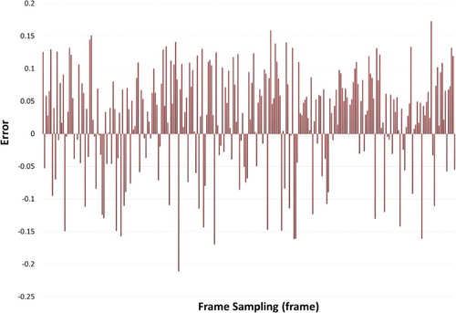
First, 25 sampling points were selected uniformly. The time estimation error was compared with those of the different methods. Error = |estimated time − actual time|/actual time. The experimental results are shown in Figure 3.

Figure 3. Comparison of method errors.

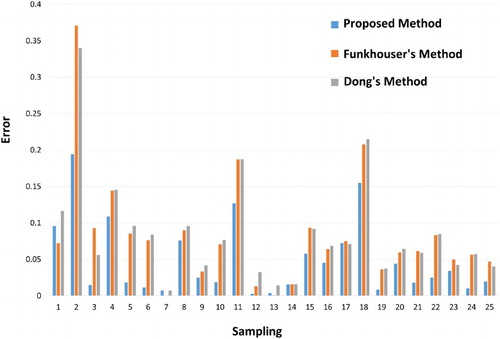
From Figure 3, we can see that the proposed method is better than the existing methods for 20 samples among the randomly selected 25 samples. In addition, the gaps in the relative errors of the remaining samples are within 0.05. Therefore, it is shown that the proposed method is more suitable for the rendering time estimation of 3D city models than the existing methods.

To verify that the proposed method can accurately estimate the rendering time in practical applications (i.e. with a continuous movement of the viewpoint), we compare the actual time with the estimated time computed by the proposed method during browsing, as is shown in Figure 4.

Figure 4. Actual times and estimated times during browsing.

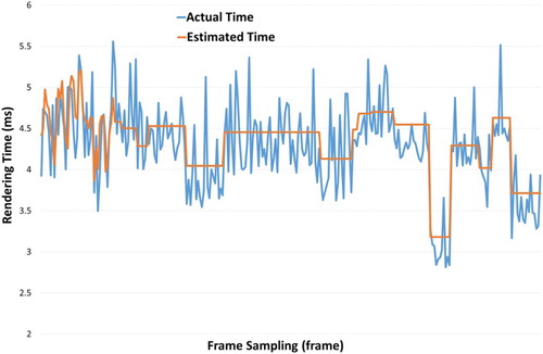
From Figure 4, we can see that the estimated time is computed based on the number of textures, the number of vertices and other parameters in the scene; therefore, the estimated time curve will become very smooth when the scene changes slightly with the slow movement of the viewpoint. However, the actual time curve will fluctuate rapidly even if the scene does not change, because the actual render time is also affected by the instability of the computer hardware. Overall, however, the estimated time is generally synchronized with the actual time.

Figure 5 shows the time estimation error recorded during the scene browsing process using the proposed method, for which the estimated error = (estimated time − actual time)/actual time.

Figure 5. Estimated errors during browsing.

From Figure 5, we can see that the error is between ±0.15, while the average of the absolute value of the error is 0.068, which satisfies the requirement for adaptive visualization. We also found that the number of positive errors is much greater than that of negative errors, which is mainly because the samples used to build the regression model were selected when the scene was initialized, and the initialization process increases the render time. During the runtime, the movement of the viewpoint is a continuous process, and partial scenes have been loaded. Therefore, the loading frequency of each scene is reduced, and the rendering time during browsing is shorter than that during the initialization. The main reason for intermittent negative errors may be that large changes in the scenes may lead to sudden frame drops.

4.2. Scene optimization

To verify that the scene optimization algorithm provides a better visual effect and optimization convergence speed than the existing methods, we designed the following experiment (the experiments were carried out on a Dell computer with a 3.10 GHz CPU, 8 GB of RAM, and a 640 MHz GPU).

The existing adaptive visualization methods (Zhang, Zhu, and Hu 2007; Sunshine-Hill 2013; Dong et al. 2015) are essentially based on a greedy algorithm (Funkhouser and Séquin 1993), which traverses the objects in order of importance to optimize the scene, and they do not make many improvements to Funkhouser’s method. Thus, the method described in this paper is mainly compared with Funkhouser’s method.

Figures 6–8 compare the visual effects of a scene obtained using the proposed method and an existing method. Figure 6 shows the visual effect when the scene is not optimized. Figure 7 shows the visual effect after using Funkhouser’s optimization method, and Figure 8 shows the visual effect after using the proposed method.

Figure 6. Original visual effect.

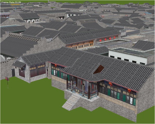
Figure 7. Visual effect after using Funkhouser’s optimization method.

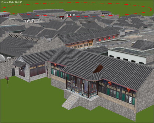
Figure 8. Visual effect after using the proposed method.

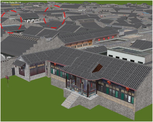
From Figures 6–8, we can see that the proposed method and Funkhouser’s method both increase the frame rate from 50 to 100 FPS after optimization. However, Funkhouser’s optimization method results in the loss of many distant buildings (within the circle in Figure 7). The proposed method pays more attention to the overall features of the scene. Although the circles in Figure 8 indicate a more significant visual loss, the overall visual effect is not very different from that shown in Figure 6.

Figure 9 compares the convergence speed of the scene optimization algorithm of the proposed method with that of Funkhouser’s method.

Figure 9. Comparison of optimization times.

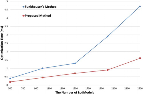
The experimental results in Figure 9 mainly record the convergence times of the optimization algorithms with respect to the different numbers of LodModels (buildings).

Compared with the existing methods, the proposed method organizes a scene based on a tiled quadtree of the virtual globe and uses Tiles instead of a single LodModel for sorting, thereby effectively improving the convergence speed of the optimization.

4.3. Adaptive visualization

To verify that the proposed visualization method can automatically optimize a 3D city scene according to the terminal hardware performance and implement optimal rendering among different hardware environments, this paper conducted experiments on three computers with different levels of performances. The computer configurations are listed in Table 1.

Table 1. Configurations of the computers.

Device	Graphics card	GPU clock (MHz)	Shaders	CPU	Memory (GB)	Operating system
Computer 1	NVS 3100 M	606	16	Intel(R) Core(TM) i7 2.67 GHz	4	Win 7 32-bit
Computer 2	GeoForce 800 M	1024	384	Intel(R) Core(TM) i5 1.70 GHz	8	Win 7 64-bit
Computer 3	Quadro 600	640	96	Intel(R) Core(TM) i3 3.10 GHz	8	Win 7 64-bit

Table 2 lists the coefficients of the render time estimation factors for the different computers (the constants c1, c2  …  c5 are described in Section 3.1).

Table 2. Coefficients of the render time estimation factors for the different computers.

Device	#tv	#pix	#matrix	#boundingbox	#texture
Computer 1	8.58E−05	3.11E−05	0.000205	0.000836	0.007907
Computer 2	6.11E−06	8.91E−06	0.000352	0.001039	0.00997
Computer 3	1.75E−05	2.59E−05	0.000284	0.000763	0.00245

From Table 2, we can see that smaller coefficients are correlated with faster processing times, as the coefficients partly reflect the ability of the computer to address different factors. According to Section 3.1, the following are observed: for the ability of Cull, Computer 3 ≈ Computer 1 > Computer 2; for the ability of draw call: Computer 3 > Computer 1 > Computer 2; and for the ability of GPU draw: Computer 2 > Computer 3 > Computer 1.

The experimental method is established as follows. A flight path is set across the entire scene, for which the total fly time is 30 s. As the flight speed is fixed, the same fly time indicates the same viewpoint position. The rendering times before and after using the proposed method are then recorded.

Figure 10 compares the rendering time on Computer 1 before and after using adaptive visualization.

Figure 10. Comparison of rendering times on Computer 1.

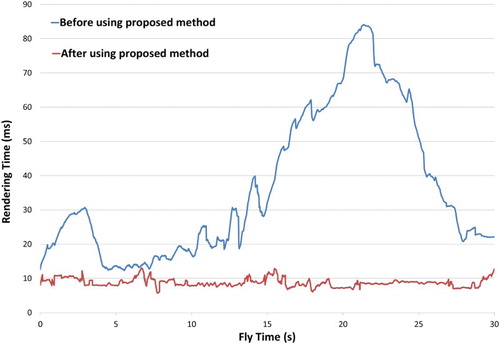
From Figure 10, we can see that the rendering time before using the proposed method exhibits dramatic increases and decreases depending on the complexity of the scene. After using the adaptive visualization method proposed in this paper, the rendering time was stabilized to the given time (10 ms).

Figure 11 compares the rendering time on Computer 2 before and after using the proposed method.

Figure 11. Comparison of rendering times on Computer 2.

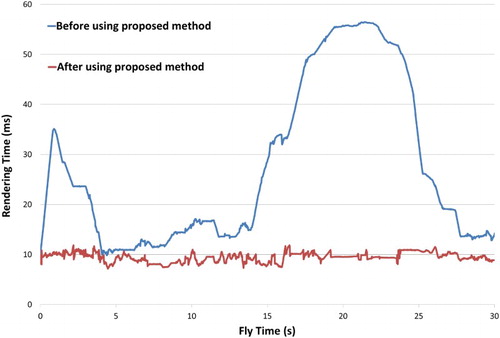
Comparing Figure 11 with Figure 10, we can see that the rendering time before using the proposed method will change with the performance of the computer, while the rendering time after using adaptive visualization will be maintained at the given time (10 ms). Thus, the proposed method effectively reduces the dependence on the computer hardware performance.

Figure 12 compares the rendering times on Computer 3 before and after using the proposed method.

Figure 12. Comparison of rendering times on Computer 3.

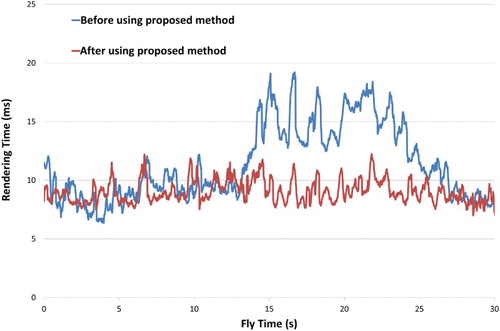
From Figure 12, we can see that, when the rendering time is shorter than the given time (10 ms), the two rendering times are similar. When it is longer than the target time, adaptive visualization can be used to optimize the scene and reduce the render time to the target time.

5. Conclusions and future work

This paper presented a 3D city model visualization method that can adapt to different levels of computer performances and achieve high-efficiency rendering with different levels of hardware performance. First, the possible rendering times for each model were estimated according to the computer CPU and GPU performances, and the LOD for each model was dynamically adjusted based on the results of the rendering time estimation to ensure that the final scene could be completed within the given time. Compared with existing adaptive visualization methods, the advantages of the proposed method are described hereafter.

In terms of estimating the rendering time, the proposed method is an extension of an existing time estimation method. The proposed method not only considers the characteristics of the data structure of the 3D city models but also avoids the influence of dynamic loading on the estimation accuracy. Therefore, the estimation accuracy is greatly improved relative to the existing method.

In terms of the scene optimization, the proposed method reorganizes the 3D city model into a tiled quadtree structure based on the idea of a global discrete grid on the virtual globe. By using tiles instead of a single model to participate in the iterative calculation, the optimized convergence time is effectively reduced. At the same time, an optimization algorithm considering the overall visual effect is proposed. The new algorithm first determines the number of rendering objects and then determines the LOD, which overcomes the problem within the existing methods whereby large numbers of rendering objects are lost.

Three experiments are implemented to prove the validity of the proposed method. (1) The first experiment shows that the rendering times computed by the proposed time estimation method are more accurate than those of the existing method, and the maximal estimation error is less than 15%. This guarantees the implementation of the subsequent scene optimization method. (2) The second experiment shows that the proposed scene optimization method is faster than the existing method in terms of the convergence speed, and the visual effects are better when the frame rate is the same as that of the existing method. (3) The third experiment shows that the proposed adaptive visualization method can adapt to different levels of computer performance and achieve high-efficiency rendering with different levels of hardware performance.

As the current 3D city model mainly consists of the shapes of buildings, and the indoor structures are relatively simple, the 3D city model can be treated as a traditional discrete LOD model. Given the ongoing development of city modeling methods, the indoor structures of models will continue to improve such that complex indoor structures will require special scene organization techniques and the application of occlusion culling technologies, thereby giving rise to higher requirements for rendering time estimations and scene optimization algorithms. As such, the latter will be the focus of our next study.

Acknowledgements

The authors appreciate the comments from the anonymous reviewers and editor.

Disclosure statement

No potential conflict of interest was reported by the authors.

ORCID

Jing Chen http://orcid.org/0000-0002-8067-0201

Additional information

Funding

This work was supported by the National Key R&D Program of China [grant number 2017YFB0503703]; The Nature Science Foundation Innovation Group Project of Hubei Province, China [grant number 2016CFA003]; The LIESMARS Special Research Funding.

References

- Chen, Jing, Tong Zhang, Shutao Dong, and Bingxiong Xie. 2014. “Fast Registration of Multisource Three-Dimensional City Models in GeoGlobe.” International Journal of Digital Earth 8 (4): 1–19. doi:10.1080/17538947.2014.885596.
- Doellner, Juergen, Benjamin Hagedorn, and Jan Klimke. 2012. “Server-Based Rendering of Large 3D Scenes for Mobile Devices Using G-Buffer Cube Maps.” Paper presented at the proceedings of the 17th international conference on 3D Web Technology, Los Angeles, CA.
- Dong, Tianyang, Siyuan Liu, Jiajia Xia, Jing Fan, and Ling Zhang. 2015. “A Time-Critical Adaptive Approach for Visualizing Natural Scenes on Different Devices.” PLoS One 10 (2): 1–26. doi:10.1371/journal.pone.0117586.
- Ellul, Claire, and Julia Altenbuchner. 2014. “Investigating Approaches to Improving Rendering Performance of 3D City Models on Mobile Devices.” Geo-spatial Information Science 17 (2): 73–84. doi:10.1080/10095020.2013.866620.
- Funkhouser, Thomas A., and Carlo H. Séquin. 1993. “Adaptive Display Algorithm for Interactive Frame Rates During Visualization of Complex Virtual Environments.” Paper presented at the proceedings of the 20th annual conference on Computer Graphics and Interactive Techniques, Anaheim, CA.
- Gobbetti, Enrico, Fabio Marton, Marcos Balsa Rodriguez, Fabio Ganovelli, and Marco Di Benedetto. 2012. “Adaptive Quad Patches: An Adaptive Regular Structure for Web Distribution and Adaptive Rendering of 3D Models.” Paper presented at the proceedings of the 17th international conference on 3D Web Technology, Los Angeles, CA.
- Hernández, Eduardo, and Bedrich Beneš. 2005. “Robin Hood’s Algorithm for Time-Critical Level of Detail.” Paper presented at the fifteenth international conference on Computer Graphics and Applications (Graphi Con’2005), Novosibirsk Akademgorodok, Russia.
- Koskela, Timo, and Jarkko Vatjus-Anttila. 2015. “Optimization Techniques for 3D Graphics Deployment on Mobile Devices.” 3D Research 6 (1): 1–27. doi:10.1007/s13319-015-0040-0.
- Krebs, Allan Meng, Ivan Marsic, and Bogdan Dorohonceanu. 2002. “Mobile Adaptive Applications for Ubiquitous Collaboration in Heterogeneous Environments.” Paper presented at the proceedings 22nd international conference on Distributed Computing Systems Workshops, Vienna, Austria.
- Lakhia, Ali. 2004. “Efficient Interactive Rendering of Detailed Models with Hierarchical Levels of Detail.” Paper presented at the proceedings 2nd international symposium on 3DPVT (3D Data Processing, Visualization and Transmission), Thessaloniki, Greece.
- Lavoué, Guillaume, Laurent Chevalier, and Florent Dupont. 2013. “Streaming Compressed 3D Data on the Web Using JavaScript and WebGL.” Paper presented at the proceedings of the 18th international conference on 3D Web Technology, San Sebastian, Spain.
- Lee, Ho, Guillaume Lavoué, and Florent Dupont. 2012. “Rate-Distortion Optimization for Progressive Compression of 3D Mesh with Color Attributes.” The Visual Computer 28 (2): 137–153. doi: 10.1007/s00371-011-0602-y
- Nijdam, N. A., S. Han, B. Kevelham, and N. Magnenat-Thalmann. 2010. “A Context-Aware Adaptive Rendering System for User-Centric Pervasive Computing Environments.” Paper presented at the Melecon 2010-2010 15th IEEE Mediterranean Electrotechnical Conference, Valletta, Malta.
- Preda, Marius, Paulo Villegas, Franciso Morán, Gauthier Lafruit, and Robert-Paul Berretty. 2008. “A Model for Adapting 3D Graphics Based on Scalable Coding, Real-Time Simplification and Remote Rendering.” The Visual Computer 24 (10): 881–888. doi: 10.1007/s00371-008-0284-2
- Sunshine-Hill, Ben. 2013. “Managing Simulation Level-of-Detail with the LOD Trader.” Paper presented at the Motion on Games, Dublin, Ireland.
- Wimmer, Michael, and Peter Wonka. 2003. “Rendering Time Estimation for Real-Time Rendering.” Paper presented at the Rendering Techniques, Leuven, Belgium.
- Yu, Zhuo, Xiaohui Liang, and Zhiyu Chen. 2008. “A Level of Detail Selection Method for Multi-Type Objects Based on the Span of Level Changed.” Paper presented at the IEEE Conference on Robotics, Automation and Mechatronics, Chengdu, China.
- Zach, Christopher, Stephan Mantler, and Konrad Karner. 2002. “Time-Critical Rendering of Discrete and Continuous Levels of Detail.” Paper presented at the proceedings of the ACM symposium on Virtual Reality Software and Technology, Hong Kong, China.
- Zhang, Liqiang, Chunming Han, Liang Zhang, Xiaokun Zhang, and Jonathan Li. 2014. “Web-Based Visualization of Large 3D Urban Building Models.” International Journal of Digital Earth 7 (1): 53–67. doi:10.1080/17538947.2012.667159.
- Zhang, Yeting, Qing Zhu, and Mingyuan Hu. 2007. “Time-Critical Adaptive Visualization Method of 3D City Models.” Paper presented at the proceedings of SPIE, Wuhan, China.