Most similar neighbor imputation of forest attributes using metrics derived from combined airborne LIDAR and multispectral sensors

ABSTRACT

In the context of predicting forest attributes using a combination of airborne LIDAR and multispectral (MS) sensors, we suggest the inclusion of normalized difference vegetation index (NDVI) metrics along with the more traditional LIDAR height metrics. Here the data fusion method consists of back-projecting LIDAR returns onto original MS images, avoiding co-registration errors. The prediction method is based on non-parametric imputation (the most similar neighbor). Predictor selection and accuracy assessment include hypothesis tests and over-fitting prevention methods. Results show improvements when using combinations of LIDAR and MS compared to using either of them alone. The MS sensor has little explanatory capacity for forest variables dependent on tree height, already well determined from LIDAR alone. However, there is potential for variables dependent on tree diameters and their density. The combination of LIDAR and MS sensors can be very beneficial for predicting variables describing forests structural heterogeneity, which are best described from synergies between LIDAR heights and NDVI dispersion. Results demonstrate the potential of NDVI metrics to increase prediction accuracy of forest attributes. Their inclusion in the predictor dataset may, however, in a few cases be detrimental to accuracy, and therefore we recommend to carefully assess the possible advantages of data fusion on a case-by-case basis.

KEYWORDS:

• Airborne laser scanning
• forest attribute prediction
• multispectral imagery
• data fusion
• nearest neighbor

1. Introduction

Methods for prediction of forest attributes assisted by light detection and ranging (LIDAR) sensors are spreading, and procedures are becoming standard (Corona and Fattorini 2008; Hollaus et al. 2009; White et al. 2013; Maltamo, Næsset, and Vauhkonen 2014). The most widespread approach is the area-based method (Næsset 2002), which consists of modeling relationships between a feature space (X) of LIDAR metrics – statistics summarizing the height distribution of returns – and stand attributes measured in the field (Y) (e.g. Hudak et al. 2006; Kronseder et al. 2012; Montaghi et al. 2013; Bottalico et al. 2017). Amid many alternatives for modeling, the most similar neighbor (MSN) (Moeur and Stage 1995) is proven to be one the most reliable choices (Packalén and Maltamo 2006; Hudak et al. 2008). MSN is one particular type among the group of nearest neighbor imputation methods (Franco-Lopez, Ek, and Bauer 2001), which consist of computing distances to reference sample plots in X. These distances may be simply calculated over the Euclidean multi-dimensional space (usually known as k-NN; McRoberts, Nelson, and Wendt 2002; McInerney et al. 2010), or the feature space may be modified according to different criteria such as the proximity matrix yielded from a random forest algorithm (Hudak et al. 2008). In particular, MSN is based on the projections from a canonical correlation analysis (CCA) as feature space (Lefsky et al. 2005; Manzanera et al. 2016). MSN is particularly well-suited for most practical situations in LIDAR-assisted forest inventories (Maltamo, Næsset, and Vauhkonen 2014).

Despite the rapid development of standard LIDAR procedures for forest inventory, combining the information of LIDAR with multispectral (MS) sensors is still far from being operational for most practitioners. The most common approach combines classification of MS imagery, to determine species mixture, with MSN imputation of forest attributes based on LIDAR metrics, to obtain species-specific results (e.g. Packalén and Maltamo 2006; Heinzel and Koch 2012; Ørka et al. 2012). One explanation for the slower development of standard procedures for forest prediction using combinations of sensors may be that achieving a proper correspondence between the datasets has proved to be a challenging task (Pohl and van Genderen 2015). Orthorectification of the MS imagery is the most common method used for data fusion (e.g. Erdody and Moskal 2010; García et al. 2011; Heinzel and Koch 2012; Latifi et al. 2012; Dupuy et al. 2013; Rezayan and Erfanifard 2016). However, there have been reports that the spatial co-registration of datasets achieved with orthorectification may be too poor (Valbuena et al. 2011; Asner et al. 2012; Torabzadeh, Morsdorf, and Schaepman 2014; Wu et al. 2015), affecting the accuracy of the estimates (McRoberts 2010; Bright, Hicke, and Hudak 2012) unless control points are added manually (García et al. 2011). An alternative are the so-called ‘true-orthorectification’ methods, which correct the positions of MS sensor information using a digital surface model instead of the digital terrain model (DTM) (Waser et al. 2008). Although true-orthorectification may obtain satisfactory accuracies in urban areas (Youn et al. 2008; Lehrbass and Wang 2012), obtaining satisfactory positional accuracies in forested environments has been reported to be a challenging task (St-Onge 2008; Valbuena et al. 2011). On the other hand, the method of projecting the LiDAR returns into the image space (also known as back-projection; Forkuo and King 2004) is an alternative to orthorectification and true-orthorectification. Back-projection makes use of the same collinearity principles as orthorectification and true-orthorectification but reduces error-prone steps, such as least-squares adjustments or resampling-based rasterization (Valbuena et al. 2011). The result is a colored point cloud that allows the use of information from both sensors, getting the most out of their potential for applications to forest inventory (Packalén, Suvanto, and Maltamo 2009; Ørka et al. 2012; Valbuena et al. 2013a).

The optimization of correspondence between LIDAR and MS sensors has enabled some improvements in the prediction of forest attributes (Lu et al. 2014). Packalén, Suvanto, and Maltamo (2009) carried out species-specific predictions incorporating the spectral information as a proxy for species mixture in the standard area-based approach. Ørka et al. (2012) showed that combining LIDAR and MS sensors may also improve results of species classification at tree level. Valbuena et al. (2013a) also observed that incorporating a metric from the MS sensor can improve predictions in monocultures for forest attributes that may be explained by variability in albedo, like stand density. Manzanera et al. (2016) explored the potential of MS sensors by computing the same array of metrics which are commonly computed for explaining the distribution of LIDAR heights (Næsset 2002; Hudak et al. 2006; White et al. 2013; Maltamo, Næsset, and Vauhkonen 2014), but applied to normalized difference vegetation index (NDVI) instead, suggesting that synergies between MS and LIDAR metrics could potentially be related to some forest structural attributes. In this article, we go a step beyond Manzanera et al. (2016), carrying out MSN predictions using a combination of LIDAR and NDVI metrics and reporting the accuracy of the final predictions. We obtained results for a wide assortment of forest attributes by combining both LIDAR and MS information, comparing the reliability of the method for each forest attribute. We also compared the accuracy of final predictions for fused LIDAR and MS sensor datasets, versus either of them alone, evaluating the gain obtained from incorporating either sensor, and synergies among them.

2. Material and methods

2.1. Study area and field information

The study area were the Scots pine-dominated (Pinus sylvestris L.) forests of Valsaín (Spain; approx. coordinates: 41°N 4°W and elevation 1300–1500 m above sea level). The field campaign consisted of a survey of 37 plots, which were composed of two concentric circles of radii 10 and 20 m radius (Valbuena et al. 2013b). For each tree, diameter at breast height (dbh, cm) was measured with a calliper and tree top heights (h, m) were determined with a Vertex III Hypsometer (Haglof, Sweden). Plot centers were staked out using a HiPer-Pro (Topcon, California) receiver set at 1–2 m above the ground for differentially-corrected global navigation satellite systems (GNSS) positioning (Valbuena et al. 2010, 2012).

Forest stand attributes and characteristics were calculated by aggregating the tree-level information into per-hectare totals at plot-level. In order to analyze different patterns of explained variability in forest characteristics by the LIDAR and MS sensors, we organized these attributes into groups containing those forest variables (I) dependent on tree diameters or (II) tree heights, (III) related to stand density and (IV) descriptors of structural heterogeneity of forests.

Variables dependent on tree diameters (Group I) were quadratic mean diameter (QMD, cm) and basal area (BA, m² ha⁻¹). The BA is the cross-sectional area occupied by trees at breast height, whereas QMD is the basal area-weighted mean tree diameter:(1) On the other hand, in Group II we included forest variables dependent on tree height: Lorey’s mean height (H_L, m), and standing volume (V, m³ ha⁻¹) (e.g. Næsset 2002). H_L is the basal area-weighted mean tree height, whereas V was aggregated from allometric predictions of individual tree stem volumes (v, m³). Locally-adjusted tree allometry specific for P. sylvestris was employed to obtain v (Rojo and Montero 1996):(2) In Group III we included two closely related attributes: stem density (N, stems ha⁻¹), and stand density index (SDI; Reineke 1933). Both describe stand density: N in absolute terms whereas SDI is relative to the size of the trees. The formula for SDI was detailed in Valbuena et al. (2013a).

Group IV were variables describing the structural heterogeneity of forests were obtained following Valbuena et al. (2014), although in this study the array of indicators was restricted to those found to provide a complete and concise description of forest structure (as reasoned in Valbuena [2015]): the Gini coefficient (GC) (Weiner and Solbrig 1984), and the proportion of basal area larger than the mean (BALM) (Gove 2004). While GC summarizes the inequality of sizes among the trees growing in vicinity, BALM can be used to describe the relative dominance among forest vertical strata and understorey development (Valbuena et al. 2013b).

2.2. Remote sensing datasets and sensor fusion

LIDAR and MS sensors were simultaneously mounted on a gyro-stabilized platform on-board a 404-Titan (Cessna, Kansas). The flight took place at an approximate altitude of 1500 m and ground speed of 72 m s⁻¹. On-flight GNSS and inertial navigation systems provided sensor position and attitude, respectively. The LIDAR sensor was an ALS50-II (Leica Geosystems, Switzerland), which at a pulse frequency of 55 kHz obtained an average pulse density of 1.15 pulses m⁻² and an approximate pulse footprint diameter of 0.5 m (Baltsavias 1999). The survey consisted of four scan lines of 665 m swath width with a 40% side lap covering an approximate total area of 800 ha. Returns were classified as ground using Terrascan’s (Terrasolid, Finland) implementation of Axelsson’s (2000) algorithm. The method iteratively densified a triangular irregular network of LIDAR ground returns by including additional returns under criteria set as lowest elevation difference = 2 m and a threshold angle = 12–75°, which assured the dismissal of vegetation, buildings, boulders, etc. (Axelsson 2000). Ground returns were interpolated into a DTM with a spatial resolution of 1 m and a precision of about 15 cm, calculated by ground quality control (Valbuena et al. 2012). Heights above ground (H, m) were computed for individual returns by subtracting the DTM value underneath.

The MS sensor consisted of a DMC camera system (Zeiss-Intergraph, Germany) composed of four CCD frames with focal length of f = 30 mm providing selective sensitivity for blue, green, red and near-infrared (NIR). These images had an approximate ground sampling distance of 60 cm (Wolf 1983). Digital numbers from the spectral bands for red and NIR were employed to obtain (non-orthorectified) images containing NDVI values calculated at pixel-level (Rouse et al. 1974). Sensor data fusion was carried out using a projection procedure which assured the correspondence between the H and NDVI information (Valbuena et al. 2011). The procedure consisted of projecting each first return from the LIDAR dataset onto the NDVI image closest to nadir, retrieving back the NDVI value of the pixel at that position (Forkuo and King 2004), which effectively resulted in a NDVI-colored LIDAR point cloud. The resulting root mean square error in co-registration of the LIDAR-MS fusion product was 0.54 m, which was mainly dependent on the spatial resolution of the MS image (Valbuena et al. 2011).

2.3. Predictor computation and MSN imputation

Using FUSION software (USDA Forest Service; McGaughey 2012), the NDVI-colored LIDAR returns corresponding to the field plots were extracted using the GNSS-surveyed plot center coordinates. We computed area-based metrics as they are typically obtained from the heights of LIDAR returns H (see e.g. Næsset 2002; White et al. 2013; Maltamo, Næsset, and Vauhkonen 2014). These metrics were an array of statistical descriptors of the distribution of LIDAR heights backscattered from that plot, such as moments, order statistics, quantiles and proportions above given thresholds (see McGaughey [2012] for a full description of metrics). In addition to these H metrics (denoted as H.xxx, where xxx refers to each given metric, see Table 1), the same descriptors for the distribution of NDVI values reflected from the field plot positions were computed, obtaining NDVI metrics (denoted as NDVI.xxx, similarly – Table 1). In this study, traditional H metrics and novel NDVI metrics were considered together for the predictions of forest attributes.

Table 1. Summary of a selection metrics computed with FUSION (McGaughey 2012).

Prefix	Suffix	Description
H./NDVI.	Mean	Mean
H./NDVI.	StdDev	Standard deviation
H./NDVI.	CV	Coefficient of variation
H./NDVI.	Skew	Skewness
H./NDVI.	IQR	Inter-quartile range
H./NDVI.	Var	Variance
H./NDVI.	L1, L2, L3, L4	L-moments
H./NDVI.	GC	Gini Coefficient (L-coefficient variation; Valbuena et al. 2017)
H./NDVI.	AAD	Average absolute deviation
H./NDVI.	P10, P20 …	Percentile values (1st, 5th, 10th, 20th, 25th, 30th, 40th, 50th,
H./NDVI.	… P80, P90	60th, 70th, 75th, 80th, 90th, 95th, 99th percentiles)

H prefix: height metrics; NDVI prefix: normalized difference vegetation index-derived metrics.

We therefore had three alternative matrices of predictors for the MSN imputation of forest variables: (i) a set of metrics describing the distribution of LIDAR heights ; (ii) another similar set of metrics derived from the NDVI values calculated from the MS sensor ; and (iii) a compiled sensor fusion dataset including both H and NDVI metrics . In the case of the response dataset, the forest attributes described above were considered as several univariate dependent variables estimated separately . For all these combinations of dependent and independent variables we carried out MSN (Moeur and Stage 1995) predictions using all the above-mentioned variables calculated at the position of the field plots as training data. These were done using the package yaImpute (version 1.0-18; Crookston and Finley 2008) for k-NN imputation in the R statistical environment (version 3.3.1; R Core Team 2011). Each feature space – , , or – was modified into projections obtained from a CCA, which compressed the original multidimensionality into few components which maximized the covariance between predictor and response. A preselection of both H and NDVI metrics was carried out according to the CCA results and hypothesis tests (see below). Then the MSN procedure computed a matrix of distances among all the field plots in the modified feature space. For each plot, the nearest k = 3 neighbors were searched among the remaining of the plots under the criterion of the shortest distances, effectively finding the MSNs. The value of k was set on the basis of previous experience (Valbuena et al. 2014). For each plot, the final imputed value was an inverse-distance weighted average of the values of Y for its MSNs.

2.4. Accuracy assessment and predictor variable selection

All the MSN predictions of forest attributes were evaluated and compared by leave-one-out cross-validation. Model training for the prediction of each field plot (i) was done without the influence of that given plot, and the whole MSN procedure was repeated for each subset containing all the field plots but the one predicted (pre_i). Comparing these predicted values against those measured in the field (observed; obs_i), we evaluated their accuracy from the mean signed difference (MSD), and their precision from the root mean squared differences (RMSD). Relative figures were also obtained as percentages with respect to the means of observations :(3) (4) (5) (6)

Also, to indicate the degree of agreement between the cross-validated predictions and the observed values, we calculated their coefficient of determination (R²) as:(7) To limit the number of variables in the final predictor dataset, they were ranked according to their CCA loadings (Manzanera et al. 2016) and selected under the criterion of RMSD minimization with two additional constraints: a hypothesis test and avoiding overfitting. Hypothesis tests were devoted to demonstrating that the regression of predicted to observed values followed the 1:1 correspondence line:(8) which was considered demonstrated by a failure to reject either null hypotheses that H₀: α = 0 and H₀: β = 1 (Piñeiro et al. 2008). Whenever any H₀ was rejected, an additional predictor was included in X according to CCA loadings, and the whole MSN procedure repeated. The additional constraint to avoid overfitting the predictions to the field sample was based on comparing the sums of squares ratio (SSR) between residuals obtained via cross-validation (SS^cv ) and those fitted using the entire sample (SS^fit ) (Snee 1977; Hawkins 2004):(9) which was set to a limit ensuring that SS^cv would not exceed 10% of original unexplained variability (i.e. SSR ≤ 1.1) (Lipovetsky 2013; Valbuena et al. 2013c). In cases where these constraints were not met, the best unconstrained plausible model is still reported in results section, for comparison purposes.

3. Results

3.1. Group I: variables dependent on tree diameter

The first group of forest attributes assessed were those directly related to the size of trees in terms of their dbh, which were QMD and BA. Table 2 summarizes the diagnosis of the jack-knife predictions obtained by MSN for this group of forest attributes, and Figure 1 compares the cross-validated predictions against the observed values obtained when using the combination of LIDAR and MS sensors . Scatterplots obtained from either sensor alone, and details of the predictors finally selected for the MSN imputation can be found in the Supplementary Material. The MSN imputation obtained unbiased predictions for these variables, since in all cases. Precision of predictions were narrower when using LIDAR variables than MS variables, however the best result always came from a combination of both. In the case of QMD, an RMSD = 27.88% was obtained from LIDAR predictors alone and an RMSD = 39.34% from MS, which were improved up to an RMSD = 23.09% obtained as a result of their combination. Similar results were observed for BA; an RMSD = 17.45% was obtained from LIDAR and RMSD = 25.62% from MS, while their combination reached RMSD = 14.02%. The SSR = 1.16 obtained from was however slightly large, showing no improvement when adding or eliminating predictor variables, which may indicate a tendency to overfit to the field sample. This could possibly be avoided by increasing the sample size. Scatterplots in Figure 1 showed evenly distributed error variances for all models, and hence residual homoscedasticity was another advantage of combining both sensors. On the other hand, when using only MS variables, all predictions obtained failed the hypothesis tests of correspondence between observed and predictors (Figure S2.1), and only the best plausible models were therefore reported in Table 2. In turn, using only LIDAR variables yielded reliable and accurate predictions, though these were in general improved when combined with variables from the MS sensor as well.

Figure 1. Observed versus predicted (cross-validated) values for Group I of structural attributes dependent on tree diameters: quadratic mean diameter and basal area, corresponding to the combination of LIDAR and MS sensors predictor dataset (LIDAR + MS in Table 2). The solid diagonal represents the 1:1 correspondence. The dashed line is the linear regression fit for , expressed on the top-left corner. (a) Quadratic mean diameter (QMD, cm) and (b) basal area (BA, m² ha⁻¹).

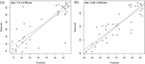
Table 2. Summary diagnosis of MSN predictions (cross-validated) for Group I of structural attributes dependent on tree diameters: quadratic mean diameter and basal area.

	Quadratic mean diameter (QMD, cm)			Basal area (BA, m^2 ha^−1)
	LIDAR	MS	LIDAR + MS	LIDAR	MS	LIDAR + MS
MSD	−0.068	0.390	−0.404	0.868	−1.483	−0.229
MSD%	−0.204	1.178	−1.220	2.077	−3.550	−0.547
RMSD	9.242	13.04	7.653	7.290	10.70	5.855
RMSD%	27.88	39.34	23.09	17.45	25.62	14.02
R^2	0.50	0.14	0.64	0.57	0.24	0.73
SSR	1.07	0.93	0.95	1.06	1.03	1.16

3.2. Group II: variables dependent on tree height

The second group of forest attributes considered were those whose calculation involved tree heights h, namely H_L and V. Results for these are summarized in Table 3, Figure 2 with details in Supplementary Material. Again, the resulting MSDs showed that all options can yield reliable results, however using variables only from the MS sensor was more prone to bias. The precision of predictions showed that while using only LIDAR variables can provide satisfactory results – with RMSD = 5.93% for H_L and RMSD = 19.90% for V – predictors derived from the MS sensor had little explanatory capacity for these forest attributes dependent on height. Thus, MS predictors yielded an RMSD = 27.18% for H_L and an RMSD = 52.25% for V. Resulting SSRs were generally low, and therefore over-fitting effects were avoided. However, MSN imputations carried out using were again unreliable, failing the hypothesis tests on the 1:1 correspondence between observed and predictions (Figure S2.2). The combination of sensors showed only very little gain – if any – comparing to predicting from alone (Table 3). Error variances were evenly distributed, especially for H_L which just required few selected LIDAR predictors to obtain very accurate predictions (Table S1.2).

Figure 2. Observed versus predicted (cross-validated) values for Group II of structural attributes dependent on tree heights: Lorey’s mean height and standing volume, corresponding to the combination of LIDAR and MS sensors predictor dataset (LIDAR + MS in Table 3). The solid diagonal represents the 1:1 correspondence. The dashed line is the linear regression fit for , expressed on the top-left corner. (a) Lorey’s height (H_L, m) and (b) standing volume (V, m³ ha⁻¹).

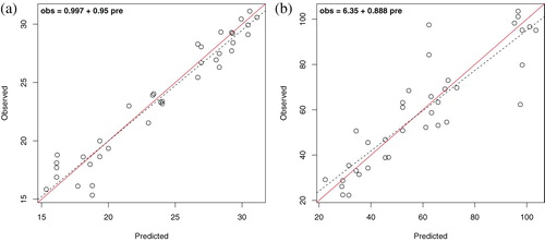
Table 3. Summary diagnosis of MSN predictions (cross-validated) for Group II of structural attributes dependent on tree heights: Lorey’s mean height and standing volume.

	Lorey’s height (HL, m)			Standing volume (V, m^3 ha^−1)
	LIDAR	MS	LIDAR + MS	LIDAR	MS	LIDAR + MS
MSD	−0.115	−1.515	0.200	−1.257	−2.190	0.373
MSD%	−0.484	−6.397	0.844	−2.112	−3.682	0.627
RMSD	1.404	6.438	1.296	11.84	31.08	11.67
RMSD%	5.930	27.18	5.471	19.90	52.25	19.62
R^2	0.92	0.44	0.94	0.78	0.01	0.77
SSR	1.03	0.99	0.98	1.05	1.10	1.05

3.3. Group III: variables related to density of trees

The third group of variables in the analysis were those related to the density of stems in the forest area. Table 4 shows the cross-validated prediction results for N and SDI, and the observed versus predicted plots obtained from are included in Figure 3. In the Supplementary Material, Table S1.3 details the predictors selected in the modeling process and Figure S2.3 the scatterplots obtained when the sensors were not combined. Although using the MS sensor alone for deriving SDI predictions showed some tendency to overestimate the relative density of a few sparsely forested areas – MSD = 9.29% (Figure S2.3(b)) – every other MSN prediction was largely unbiased. The uncertainty of the predictions for N rendered its MSN imputation model clearly unreliable for most purposes, either from , or a combination of both, failing hypothesis tests and reaching errors amounting for RMSD = 68.00% of the sample average, in the best case (Table 4). The predictions of relative stand density SDI generally obtained better results than absolute density N. An unexpected result was the observation that the combination of both LIDAR and MS sensors could only obtain a MSD = 40.90%, which in fact worsened the RMSD = 30.85% result obtained from LIDAR metrics alone. In addition, the combined dataset model for SDI also showed a slight tendency to over-fitting SSR = 1.15, which also indicates a potential damaging effect that including MS variables can have on the prediction of this particular forest variable.

Figure 3. Observed versus predicted (cross-validated) values for Group III of structural attributes related to the density of trees: stem density and stand density index, corresponding to the combination of LIDAR and MS sensors predictor dataset (LIDAR + MS in Table 4). The solid diagonal represents the 1:1 correspondence. The dashed line is the linear regression fit for , expressed on the top-left corner. (a) Stem density (N, stems·ha⁻¹) and (b) stand density index (SDI).

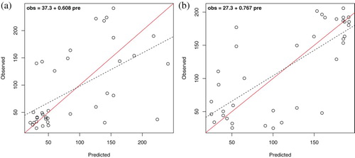
Table 4. Summary diagnosis of MSN predictions (cross-validated) for Group III of structural attributes related to the density of trees: stem density and stand density index.

	Stem density (N, stems ha^−1)			Stand density index (SDI)
	LIDAR	MS	LIDAR + MS	LIDAR	MS	LIDAR + MS
MSD	−0.162	−0.460	−1.946	2.735	−10.78	−0.461
MSD%	−0.176	−0.499	−2.115	2.359	−9.294	−0.397
RMSD	64.01	82.02	62.58	35.76	67.91	47.42
RMSD%	69.56	89.13	68.00	30.85	58.57	40.90
R^2	0.29	0.02	0.30	0.72	0.24	0.82
SSR	0.99	0.89	1.06	0.91	0.97	1.15

3.4. Group IV: variables describing structural heterogeneity

The last group of forest attributes considered were related to forest structure, in particular the heterogeneity of tree sizes and the Lorenz curve. Table 5 summarizes the results obtained for GC and BALM, and Table S1.4 details the predictors that were automatically selected in the modeling procedure. Figure 4 shows the observed versus predicted plots obtained when the LIDAR and MS sensors were combined, whereas Table S2.4 shows the results yielded by either of them alone. In spite of reaching from LIDAR and from MS in predicting GC, no major biasing problems were found. Hypothesis tests were passed, and low values for SSR indicated no over-fitting problems in the prediction. Nevertheless, R² between observed and predicted were low in most cases, with the only exception of predicting GC from the combined dataset . The accuracy of the estimates largely improved in both cases when the sensors were combined, narrowing precisions to RMSD = 45.12% for GC and RMSD = 13.57% for BALM.

Figure 4. Observed versus predicted (cross-validated) values for Group IV of forest variables describing structural heterogeneity: the Gini coefficient and the proportion of basal area larger than the mean, corresponding to the combination of LIDAR and MS sensors predictor dataset (LIDAR + MS in Table 5). The solid diagonal represents the 1:1 correspondence. The dashed line is the linear regression fit for , expressed on the top-left corner. (a) Gini coefficient (GC) and (b) basal area larger than the mean (BALM).

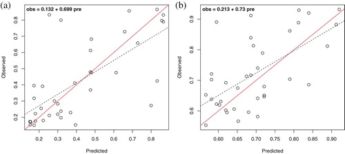
Table 5. Summary diagnosis of MSN predictions (cross-validated) for Group IV of forest variables describing structural heterogeneity: the Gini coefficient and the proportion of basal area larger than the mean.

	Gini coefficient (GC)			Basal area larger than the mean (BALM)
	LIDAR	MS	LIDAR + MS	LIDAR	MS	LIDAR + MS
MSD	−0.040	0.028	−0.004	−0.016	−0.007	−0.025
MSD%	−9.368	6.476	−1.085	−2.265	−0.927	−3.454
RMSD	0.239	0.292	0.192	0.123	0.142	0.098
RMSD%	56.14	68.60	45.12	17.09	19.69	13.57
R^2	0.21	0.06	0.45	0.09	0.05	0.37
SSR	1.02	0.99	0.98	1.05	1.09	1.06

4. Discussion

The MSN method produced the most accurate predictions for variables related to tree heights (Group II), and then to those dependent on tree diameters (Group I). In these groups, the nearest neighbor imputation method generally obtained reliable estimates, with low RMSD and high R², whenever LIDAR variables were involved in the prediction (Tables 2 and 3). The best results overall were obtained for these forest attributes, and therefore the outlined methodology for combining LIDAR and MS sensors can result in reliable estimates for these types of variables, and others alike. These results are in line with previous area-based predictions using fusion of LIDAR and MS sensors (Packalén, Suvanto, and Maltamo 2009; Erdody and Moskal 2010; García et al. 2011; Heinzel and Koch 2012; Latifi et al. 2012; Valbuena et al. 2013a; Lu et al. 2014; Su, Ma, and Guo 2017), therefore expanding the possibilities of state-of-the-art methodologies operationally employing LIDAR alone (Næsset 2002; Corona and Fattorini 2008; Hudak et al. 2008; Kronseder et al. 2012; Montaghi et al. 2013; White et al. 2013; Maltamo, Næsset, and Vauhkonen 2014; Bottalico et al. 2017). In contrast to common alternatives using orthorectification (e.g. Erdody and Moskal 2010; García et al. 2011; Heinzel and Koch 2012; Dupuy et al. 2013), the sensor fusion method by projection of the LIDAR returns into the image space has been demonstrated to achieve better correspondence for sensor information (Valbuena et al. 2011), increasing the signal-to-noise ratio in the prediction models employed (McRoberts 2010). Our results show that many metrics derived from the MS sensor can be employed to assist the prediction by incorporation inside the common LIDAR workflow, expanding the possibilities of using them from the classification suggested by Packalén, Suvanto, and Maltamo (2009) toward direct prediction (Valbuena et al. 2013a). Also, the MSN method employed in this study overcame some limitations found in the parametric models carried out by Valbuena et al. (2013a). For instance, our method incorporated the explanatory capacity of several metrics derived from the MS sensor (Saremi et al. 2014; Manzanera et al. 2016), which expanded the predictor dataset into a large array. However, this dataset can be managed by the algorithms for MSN imputation showed in this study.

In the case of forest attributes related to stand density (Group III), and therefore related to canopy cover fraction, we noticed that the predictive potential for the method was much lower when estimating the absolute number of stems growing per hectare (N), whereas stand density relative to the amount of stocking (SDI) produced more reliable estimations (Table 4). Although the estimations for both N and SDI were mostly unbiased, residuals showed very high heteroscedasticity in the case of N, for which the residual variance was much greater when N was higher (Figure 3(a)), and its resulting RMSD was consequently unreliable. The cause for this was the lack of agreement between observed and predicted values, especially for N. The overall diagnosis for this group of variables is that estimates related to stem density from combined LIDAR and MS sensors can be reliable when measured relative to the total stocking (SDI), but not in terms of absolute stand density. Valbuena et al. (2013a) also observed that an additional term from MS sensors would have more explanatory potential for SDI and N. These results carried out with many more metrics from MS and non-parametric regression seem to corroborate that the difference between NIR and red bands can be better related to relative density than to the absolute number of stems per hectare (Saremi et al. 2014). Nonetheless, the difficulties in the prediction of N in comparison to other forest attributes is a common outcome in both LIDAR (e.g. Hyyppä et al. 2000; Næsset 2002; Hudak et al. 2006; Hollaus et al. 2009; White et al. 2013; Maltamo, Næsset, and Vauhkonen 2014) and MS-assisted prediction (Franco-Lopez, Ek, and Bauer 2001). More research would therefore be needed to improve the capacity of these sensors to reliably estimate absolute stem density, given the importance of these variables for preventing and monitoring illegal logging (d’Oliveira et al. 2012). Some suggestions for improvement could be to research the explanatory capacity of textural metrics (Packalén and Maltamo 2006) or tree-level approaches (Koukoulas and Blackburn 2005; Ørka et al. 2012), perhaps considering a comparison of alternative NDVI metrics derived from either the original bands or pansharpened imagery (Valbuena et al. 2011; Chen, Hay, and St-Onge 2012).

Regarding the group of forest structure attributes based on the Lorenz curve of tree size inequality (Group IV), we obtained less positive results than expected. The results for RMSD and R² were sub-optimal, except for the combined LIDAR + MS prediction for GC (Table 5). This result was expected, given an earlier multivariate exploratory analysis (Manzanera et al. 2016). The MSN predictions further obtained in this study indicate that combining LIDAR and MS sensors can improve remote sensing predictions of forest structural heterogeneity. A closer look at the selected predictors (Table S1.4) can provide an explanation on the synergistic explanatory capacity of these variables. The model using only LIDAR variables is mainly relying on L-moments, which is convergent with results observed in boreal forests where P. sylvestris is also the main dominant species (Valbuena et al. 2016, 2017). In the case of GC prediction using , the final selection was limited to predictors describing the average LIDAR height in combination with NDVI dispersion. Therefore, structural heterogeneity is possibly determined by these two synergic factors. Figure 4(a) shows that GC predictions greatly improved from the combination of both sensors, which otherwise fitted rather poorly on their own. Therefore, given the results obtained in this study, we state that the incorporation of metrics from MS sensors can be beneficial to the accuracy in the prediction of the GC of tree size inequality. In this study we chose to accompany GC with BALM, a forest variable employed for describing the relative development of understorey with respect to the overstorey (Gove 2004), and hence a descriptor of the asymmetry of the Lorenz curve (Valbuena 2015). All the MSN imputation models obtained accurate predictions for BALM, the forest attribute describing the shape of the Lorenz curve of tree basal areas, and therefore describing the relations of relative dominance among forest vertical strata. The accuracy obtained, with RMSD = 13.57% (Table 4) was similar to the values reported for the prediction of forest attributes from the Group I (Table 2), which was also an expected result in light of findings by Manzanera et al. (2016). Thus, the combination of predictors from LIDAR and MS sensors using the current state-of-the-art in sensor data fusion can improve the prediction of variables describing forest structural heterogeneity, GC and BALM.

5. Conclusions

In this research we explored the potential for improving the accuracy of predictions of forest attributes by incorporating a set of predictors describing the distribution of NDVI values obtained from a MS sensor, and adding it to those more commonly used from LIDAR. Results showed that, although NDVI metrics have little explanatory capacity by themselves, they may assist in improving and fine-tuning those obtained by LIDAR alone, exploiting synergistic capabilities between the two sensors. We observed that the MS sensor has little explanatory capacity for forest variables dependent on tree height, which are already well determined from LIDAR alone. However, variables dependent on tree diameters and the density of stems might be better predicted by a combination of LIDAR and MS data. The inclusion of MS sensors to predict relative density may however be detrimental to obtaining reliable results, and therefore the incorporation of MS predictors should always be considered in an individual basis. On the other hand, we observed that the combination of LIDAR and MS sensors can be very beneficial for predicting variables rendering the structural heterogeneity of forests, which may be best described from synergies between LIDAR heights and dispersion of NDVI values.

Acknowledgements

The authors wish to thank Jonathan Williams (University of Cambridge) for English language revision of our manuscript, and also for the comments and suggestions from the editor and two anonymous reviewers. We also thank the Valsain Forest Center, of the National Park Body (Spain), for their valuable help.

Disclosure statement

No potential conflict of interest was reported by the authors.

Additional information

Funding

This work was partially supported by the Spanish Directorate General for Scientific and Technical Research (Ministerio de Economía y Competitividad) [grant number CGL2013-46387-C2-2-R]. Ruben Valbuena’s work is supported by an H2020 Marie Sklodowska Curie Actions entitled ‘Classification of forest structural types with LIDAR remote sensing applied to study tree size-density scaling theories’ [grant number LORENZLIDAR-658180].

References

- Asner, G. P., D. E. Knapp, J. Boardman, R. O. Green, T. Kennedy-Bowdoin, M. Eastwood, R. E. Martin, C. Anderson, and C. B. Field. 2012. “Carnegie Airborne Observatory-2: Increasing Science Data Dimensionality via High-Fidelity Multi-Sensor Fusion.” Remote Sensing of Environment 124: 454–465. doi: 10.1016/j.rse.2012.06.012
- Axelsson, P. 2000. “DEM Generation from Laser Scanner Data Using Adaptive TIN Models.” International Archives of Photogrammetry and Remote Sensing 33 (Part B4): 110–117.
- Baltsavias, E. P. 1999. “Airborne Laser Scanning: Basic Relations and Formulas.” ISPRS Journal of Photogrammetry and Remote Sensing 54 (2-3): 199–214. doi: 10.1016/S0924-2716(99)00015-5
- Bottalico, F., G. Chirici, R. Giannini, S. Mele, M. Mura, M. Puxeddu, R. E. McRoberts, R. Valbuena, and D. Travaglini. 2017. “Modeling Mediterranean Forest Structure Using Airborne Laser Scanning Data.” International Journal of Applied Earth Observation and Geoinformation 57: 145–153. doi: 10.1016/j.jag.2016.12.013
- Bright, B. C., J. A. Hicke, and A. T. Hudak. 2012. “Estimating Aboveground Carbon Stocks of a Forest Affected by Mountain Pine Beetle in Idaho Using Lidar and Multispectral Imagery.” Remote Sensing of Environment 124: 270–281. doi: 10.1016/j.rse.2012.05.016
- Chen, G., G. J. Hay, and B. St-Onge. 2012. “A GEOBIA Framework to Estimate Forest Parameters from Lidar Transects, Quickbird Imagery and Machine Learning: A Case Study in Quebec, Canada.” International Journal of Applied Earth Observation and Geoinformation 15: 28–37. doi: 10.1016/j.jag.2011.05.010
- Corona, P., and L. Fattorini. 2008. “Area-based Lidar-Assisted Estimation of Forest Standing Volume.” Canadian Journal of Forest Research 38: 2911–2916. doi: 10.1139/X08-122
- Crookston, N. L., and A. O. Finley. 2008. “YaImpute: An R Package for kNN Imputation.” Journal of Statistical Software 23 (10): 1–16. doi: 10.18637/jss.v023.i10
- d’Oliveira, M. V. N., S. E. Reutebuch, R. J. McGaughey, and H. E. Andersen. 2012. “Estimating Forest Biomass and Identifying Low-Intensity Logging Areas Using Airborne Scanning Lidar in Antimary State Forest, Acre State, Western Brazilian Amazon.” Remote Sensing of Environment 124: 479–491. doi: 10.1016/j.rse.2012.05.014
- Dupuy, S., G. Lainé, J. Tassin, and J. Sarrailh. 2013. “Characterization of the Horizontal Structure of the Tropical Forest Canopy Using Object-Based LiDAR and Multispectral Image Analysis.” International Journal of Applied Earth Observation and Geoinformation 25: 76–86. doi: 10.1016/j.jag.2013.04.001
- Erdody, T. L., and L. M. Moskal. 2010. “Fusion of LiDAR and Imagery for Estimating Forest Canopy Fuels.” Remote Sensing of Environment 114: 725–737. doi: 10.1016/j.rse.2009.11.002
- Forkuo, E., and B. King. 2004. “Automatic Fusion of Photogrammetric Imagery and Laser Scanner Point Clouds.” International Archives of Photogrammetry and Remote Sensing 35: 921–926.
- Franco-Lopez, H., A. R. Ek, and M. E. Bauer. 2001. “Estimation and Mapping of Forest Stand Density, Volume, and Cover Type Using the k-Nearest Neighbors Method.” Remote Sensing of Environment 77 (3): 251–274. doi: 10.1016/S0034-4257(01)00209-7
- García, M., D. Riaño, E. Chuvieco, J. Salas, and F. M. Danson. 2011. “Multispectral and LiDAR Data Fusion for Fuel Type Mapping Using Support Vector Machine and Decision Rules.” Remote Sensing of Environment 115: 1369–1379. doi: 10.1016/j.rse.2011.01.017
- Gove, J. H. 2004. “Structural Stocking Guides: A New Look at an Old Friend.” Canadian Journal of Forest Research 34 (5): 1044–1056. doi: 10.1139/x03-272
- Hawkins, D. M. 2004. “The Problem of Overfitting.” Journal of Chemical Information and Computer Sciences 44 (1): 1–12. doi: 10.1021/ci0342472
- Heinzel, J., and B. Koch. 2012. “Investigating Multiple Data Sources for Tree Species Classification in Temperate Forest and Use for Single Tree Delineation.” International Journal of Applied Earth Observation and Geoinformation 18: 101–110. doi: 10.1016/j.jag.2012.01.025
- Hollaus, M., W. Dorigo, W. Wagner, K. Schadauer, B. Höfle, and B. Maier. 2009. “Large-area Growing Stock Estimation Based on Airborne Laser Scanning and National Forest Inventory Data.” International Journal of Remote Sensing 30 (19): 5159–5175. doi: 10.1080/01431160903022894
- Hudak, A. T., N. L. Crookston, J. S. Evans, M. J. Falkowski, A. M. S. Smith, P. E. Gessler, and P. Morgan. 2006. “Regression Modeling and Mapping of Coniferous Forest Basal Area and Tree Density from Discrete-Return Lidar and Multispectral Satellite Data.” Canadian Journal of Remote Sensing 32: 126–138. doi: 10.5589/m06-007
- Hudak, A. T., N. L. Crookston, J. S. Evans, D. E. Hall, and M. J. Falkowski. 2008. “Nearest Neighbor Imputation of Species-Level, Plot-Scale Forest Structure Attributes from LiDAR Data.” Remote Sensing of Environment 112: 2232–2245. doi: 10.1016/j.rse.2007.10.009
- Hyyppä, J., H. Hyyppä, M. Inkinen, M. Engdahl, S. Linko, and Y. Zhu. 2000. “Accuracy Comparison of Various Remote Sensing Data Sources in the Retrieval of Forest Stand Attributes.” Forest Ecology and Management 128: 109–120. doi: 10.1016/S0378-1127(99)00278-9
- Koukoulas, S., and G. A. Blackburn. 2005. “Mapping Individual Tree Location, Height and Species in Broadleaved Deciduous Forest Using Airborne LIDAR and Multi-Spectral Remotely Sensed Data.” International Journal of Remote Sensing 26: 431–455. doi: 10.1080/0143116042000298289
- Kronseder, K., U. Ballhorn, V. Böhm, and F. Siegert. 2012. “Above Ground Biomass Estimation Across Forest Types at Different Degradation Levels in Central Kalimantan Using Lidar Data.” International Journal of Applied Earth Observation and Geoinformation 18: 37–48. doi: 10.1016/j.jag.2012.01.010
- Latifi, H., A. Nothdurft, C. Straub, and B. Koch. 2012. “Modelling Stratified Forest Attributes Using Optical/Lidar Features in a Central European Landscape.” International Journal of Digital Earth 5 (2): 106–132. doi: 10.1080/17538947.2011.583992
- Lefsky, M. A., A. T. Hudak, W. B. Cohen, and S. A. Acker. 2005. “Patterns of Covariance Between Forest Stand and Canopy Structure in the Pacific Northwest.” Remote Sensing of Environment 95: 517–531. doi: 10.1016/j.rse.2005.01.004
- Lehrbass, B., and J. Wang. 2012. “Urban Tree Cover Mapping with Relief-Corrected Aerial Imagery and Lidar.” Photogrammetric Engineering & Remote Sensing 78: 473–484. doi: 10.14358/PERS.78.5.473
- Lipovetsky, S. 2013. “How Good is Best? Multivariate Case of Ehrenberg-Weisberg Analysis of Residual Errors in Competing Regressions.” Journal of Modern Applied Statistical Methods 12 (2), Article 14. doi: 10.22237/jmasm/1383279180
- Lu, D., Q. Chen, G. Wang, L. Liu, G. Li, and E. Moran. 2014. “A Survey of Remote Sensing-Based Aboveground Biomass Estimation Methods in Forest Ecosystems.” International Journal of Digital Earth 9 (1): 1–43.
- Maltamo, M., E. Næsset, and J. Vauhkonen. 2014. Forestry Applications of Airborne Laser Scanning – Concepts and Case Studies. Managing Forest Ecosystems 27. Dordrecht: Springer.
- Manzanera, J. A., A. García-Abril, C. Pascual, R. Tejera, S. Martín-Fernández, T. Tokola, and R. Valbuena. 2016. “Fusion of Airborne LIDAR and Multispectral Sensors Reveals Synergic Capabilities in Forest Structure Characterization.” GIScience & Remote Sensing 53 (6): 723–738. doi: 10.1080/15481603.2016.1231605
- McGaughey, R. J. 2012. FUSION/LDV: Software for LIDAR Data Analysis and Visualization. Version 3.10. Seattle, WA: Pacific Northwest Research Station. USDA Forest Service.
- McInerney, D. O., J. Suárez, R. Valbuena, and M. Nieuwenhuis. 2010. “Forest Canopy Height Retrieval Using Lidar Data, Medium-Resolution Satellite Imagery and kNN Estimation in Aberfoyle, Scotland.” Forestry 83 (2): 195–206. doi: 10.1093/forestry/cpq001
- McRoberts, R. E. 2010. “The Effects of Rectification and Global Positioning System Errors on Satellite Image-Based Estimates of Forest Area.” Remote Sensing of Environment 114 (8): 1710–1717. doi: 10.1016/j.rse.2010.03.001
- McRoberts, R. E., M. D. Nelson, and D. G. Wendt. 2002. “Stratified Estimation of Forest Area Using Satellite Imagery, Inventory Data, and the k-Nearest Neighbors Technique.” Remote Sensing of Environment 82: 457–468. doi: 10.1016/S0034-4257(02)00064-0
- Moeur, M., and A. R. Stage. 1995. “Most Similar Neighbor: An Improved Sampling Inference Procedure for Natural Resource Planning.” Forest Science 41 (2): 337–359.
- Montaghi, A., P. Corona, M. Dalponte, D. Gianelle, G. Chirici, and H. Olsson. 2013. “Airborne Laser Scanning of Forest Resources: An Overview of Research in Italy as a Commentary Case Study.” International Journal of Applied Earth Observation and Geoinformation 23: 288–300. doi: 10.1016/j.jag.2012.10.002
- Næsset, E. 2002. “Predicting Forest Stand Characteristics with Airborne Scanning Laser Using a Practical Two-Stage Procedure and Field Data.” Remote Sensing of Environment 80 (1): 88–99. doi: 10.1016/S0034-4257(01)00290-5
- Ørka, H. O., T. Gobakken, E. Næsset, L. Ene, and V. Lien. 2012. “Simultaneously Acquired Airborne Laser Scanning and Multispectral Imagery for Individual Tree Species Identification.” Canadian Journal of Remote Sensing 38: 125–138. doi: 10.5589/m12-021
- Packalén, P., and M. Maltamo. 2006. “Predicting the Plot Volume by Tree Species Using Airborne Laser Scanning and Aerial Photographs.” Forest Science 52: 611–622.
- Packalén, P., A. Suvanto, and M. Maltamo. 2009. “A Two Stage Method to Estimate Species-Specific Growing Stock.” Photogrammetric Engineering & Remote Sensing 75: 1451–1460. doi: 10.14358/PERS.75.12.1451
- Piñeiro, G., S. Perelman, J. P. Guerschman, and J. M. Paruelo. 2008. “How to Evaluate Models: Observed vs. Predicted or Predicted vs. Observed?” Ecological Modelling 216 (3): 316–322. doi: 10.1016/j.ecolmodel.2008.05.006
- Pohl, C., and J. L. van Genderen. 2015. “Remote Sensing Image Fusion: An Update in the Context of Digital Earth.” International Journal of Digital Earth 7 (2): 158–172. doi: 10.1080/17538947.2013.869266
- R Core Team. 2011. “R: A Language and Environment for Statistical Computing.” R Foundation for Statistical Computing, Vienna, Austria. http://www.R-project.org/.
- Reineke, L. H. 1933. “Perfecting a Stand-Density Index for Even-Aged Forests.” Journal of Agricultural Research 46: 627–638.
- Rezayan, F., and Y. Erfanifard. 2016. “Estimating Biophysical Parameters of Persian Oak Coppice Trees Using Ultracam-D Airborne Imagery in Zagros Semi-Arid Woodlands.” Journal of Arid Environments 133: 10–18. doi: 10.1016/j.jaridenv.2016.05.002
- Rojo, A., and G. Montero. 1996. El Pino Silvestre en la Sierra de Guadarrama. Madrid: Ministerio de Agricultura Pesca y Alimentación. [in Spanish].
- Rouse, J. W, R. H. Haas, J. A. Scheel and D.W. Deering. 1974. “Monitoring Vegetation Systems in the Great Plains with ERTS.” Proceedings, 3rd Earth Resource Technology Satellite (ERTS) symposium, 1: 48–62.
- Saremi, H., L. Kumar, R. Turner, C. Stone, and G. Melville. 2014. “DBH and Height Show Significant Correlation with Incoming Solar Radiation: A Case Study of a Radiata Pine (Pinus Radiata D. Don) Plantation in New South Wales, Australia.” GIScience & Remote Sensing 51: 427–444. doi: 10.1080/15481603.2014.937901
- Snee, R. 1977. “Validation of Regression Models: Methods and Examples.” Technometrics 19 (4): 415–428. doi: 10.1080/00401706.1977.10489581
- St-Onge, B. A. 2008. “Methods for Improving the Quality of a True Orthomosaic of Vexcel UltraCam Images Created Using a Lidar Digital Surface Model.” In Proceedings of SilviLaser 2008: 8th International Conference on LiDAR Applications in Forest Assessment and Inventory, edited by R. A. Hill, J. Rosette, and J. Suárez, 555–562. Edinburg: Silvilaser.
- Su, Y., Q. Ma, and Q. Guo. 2017. “Fine-Resolution Forest Tree Height Estimation Across the Sierra Nevada Through the Integration of Spaceborne Lidar, Airborne LiDAR, and Optical Imagery.” International Journal of Digital Earth 10 (3): 307–323. doi: 10.1080/17538947.2016.1227380
- Torabzadeh, H., F. Morsdorf, and M. E. Schaepman. 2014. “Fusion of Imaging Spectroscopy and Airborne Laser Scanning Data for Characterization of Forest Ecosystems - A Review.” ISPRS Journal of Photogrammetry and Remote Sensing 97: 25–35. doi: 10.1016/j.isprsjprs.2014.08.001
- Valbuena, R. 2015. “Forest Structure Indicators Based on Tree Size Inequality and their Relationships to Airborne Laser Scanning.” Dissertationes Forestales 205. Vantaa: Finnish Society of Forest Sciences.
- Valbuena, R., A. De Blas, S. Martín Fernández, M. Maltamo, G. J. Nabuurs, and J. A. Manzanera. 2013a. “Within-species Benefits of Back-Projecting Airborne Laser Scanner and Multispectral Sensors in Monospecific Pinus sylvestris Forests.” European Journal of Remote Sensing 46: 491–509. doi: 10.5721/EuJRS20134629
- Valbuena, R., K. Eerikäinen, P. Packalen, and M. Maltamo. 2016. “Gini Coefficient Predictions from Airborne Lidar Remote Sensing Display the Effect of Management Intensity on Forest Structure.” Ecological Indicators 60: 574–585. doi: 10.1016/j.ecolind.2015.08.001
- Valbuena, R., M. Maltamo, S. Martín-Fernández, P. Packalen, C. Pascual, and G. J. Nabuurs. 2013c. “Patterns of Covariance Between Airborne Laser Scanning Metrics and Lorenz Curve Descriptors of Tree Size Inequality.” Canadian Journal of Remote Sensing 39 (S1): S18–S31. doi: 10.5589/m13-012
- Valbuena, R., M. Maltamo, L. Mehtätalo, and P. Packalen. 2017. “Key Structural Features of Boreal Forests May Be Detected Directly Using L-Moments from Airborne Lidar Data.” Remote Sensing of Environment 194: 437–446. doi: 10.1016/j.rse.2016.10.024
- Valbuena, R., F. Mauro, F. Arjonilla, and J. A. Manzanera. 2011. “Comparing Airborne Laser Scanning-Imagery Fusion Methods Based on Geometric Accuracy in Forested Areas.” Remote Sensing of Environment 115: 1942–1954. doi: 10.1016/j.rse.2011.03.017
- Valbuena, R., F. Mauro, R. Rodriguez-Solano, and J. A. Manzanera. 2010. “Accuracy and Precision of GPS Receivers Under Forest Canopies in a Mountainous Environment.” Spanish Journal of Agricultural Research 8 (4): 1047–1057. doi: 10.5424/sjar/2010084-1242
- Valbuena, R., F. Mauro, R. Rodriguez-Solano, and J. A. Manzanera. 2012. “Partial Least Squares for Discriminating Variance Components in Global Navigation Satellite Systems Accuracy Obtained Under Scots Pine Canopies.” Forest Science 58 (2): 139–153. doi: 10.5849/forsci.10-025
- Valbuena, R., P. Packalen, L. Mehtätalo, A. García-Abril, and M. Maltamo. 2013b. “Characterizing Forest Structural Types and Shelterwood Dynamics from Lorenz-Based Indicators Predicted by Airborne Laser Scanning.” Canadian Journal of Forest Research 43: 1063–1074. doi: 10.1139/cjfr-2013-0147
- Valbuena, R., J. Vauhkonen, P. Packalén, J. Pitkanen, and M. Maltamo. 2014. “Comparison of Airborne Laser Scanning Methods for Estimating Forest Structure Indicators Based on Lorenz Curves.” ISPRS Journal of Photogrammetry and Remote Sensing 95: 23–33. doi: 10.1016/j.isprsjprs.2014.06.002
- Waser, L. T., E. P. Baltsavias, K. Ecker, H. Eisenbeiss, E. Feldmeyer-Christe, C. Ginzler, M. Küchler, and L. Zhang. 2008. “Assessing Changes of Forest Area and Shrub Encroachment in a Mire Ecosystem Using Digital Surface Models and CIR Aerial Images.” Remote Sensing of Environment 112: 1956–1968. doi: 10.1016/j.rse.2007.09.015
- Weiner, J., and O. Solbrig. 1984. “The Meaning and Measurement of Size Hierarchies in Plant Populations.” Oecologia 61: 334–336. doi: 10.1007/BF00379630
- White, J. C., M. A. Wulder, A. Varhola, M. Vastaranta, N. Coops, B. D. Cook, D. Pitt, and M. Woods. 2013. A Best Practices Guide for Generating Forest Inventory Attributes from Airborne Laser Scanning Data Using an Area-Based Approach. Information Report FI-X-010. Victoria, British Columbia: Canadian Forest Service, Canadian Wood Fibre Centre.
- Wolf, P. R. 1983. Elements of Photogrammetry, with Air Photo Interpretation and Remote Sensing. New York: McGraw-Hill.
- Wu, B., S. Tang, Q. Zhu, K. Y. Tong, H. Hu, and G. Li. 2015. “Geometric Integration of High-Resolution Satellite Imagery and Airborne LiDAR Data for Improved Geopositioning Accuracy in Metropolitan Areas.” ISPRS Journal of Photogrammetry and Remote Sensing 109: 139–151. doi: 10.1016/j.isprsjprs.2015.09.006
- Youn, J., J. S. Bethel, E. M. Mikhail, and C. Lee. 2008. “Extracting Urban Road Networks from High-Resolution True Orthoimage and Lidar.” Photogrammetric Engineering & Remote Sensing 74 (2): 227–237. doi: 10.14358/PERS.74.2.227