
ABSTRACT
Crop type data are an important piece of information for many applications in agriculture. Extracting crop type using remote sensing is not easy because multiple crops are usually planted into small parcels with limited availability of satellite images due to weather conditions. In this research, we aim at producing crop maps for areas with abundant rainfall and small-sized parcels by making full use of Landsat 8 and HJ-1 charge-coupled device (CCD) data. We masked out non-vegetation areas by using Landsat 8 images and then extracted a crop map from a long-term time-series of HJ-1 CCD satellite images acquired at 30-m spatial resolution and two-day temporal resolution. To increase accuracy, four key phenological metrics of crops were extracted from time-series Normalized Difference Vegetation Index curves plotted from the HJ-1 CCD images. These phenological metrics were used to further identify each of the crop types with less, but easier to access, ancillary field survey data. We used crop area data from the Jingzhou statistical yearbook and 5.8-m spatial resolution ZY-3 satellite images to perform an accuracy assessment. The results show that our classification accuracy was 92% when compared with the highly accurate but limited ZY-3 images and matched up to 80% to the statistical crop areas.
1. Introduction
Accurate and timely information on crop area statistics are important for studies of agriculture, policy, and economics, as well as hydrologic and biogeochemical processes (Ozdogan and Woodcock Citation2006). Knowing the area and types of planted crops within a country is significant information for a nation’s decision-makers when making policies regarding its food market. Specifically, crop classifications are useful in predicting crop production (Blaes, Vanhalle, and Defourny Citation2005; Wu et al. Citation2014), estimating regional crop water consumption (Stehman and Milliken Citation2007), and assessing food shortages (Zhang et al. Citation2017). Therefore, regional-scale analyses of food security and agricultural resource management require the ability to dependably map crop types (Xiao et al. Citation2005; Kumar et al. Citation2017).
Crop type information is traditionally acquired through routine reports from surveys and communication with the local farmers at the crop fields selected by the administrative inspectors (Peña-Barragán et al. Citation2011; Zhong Citation2012). However, these field-based methods are labour intensive and less effective at revealing spatial patterns at large scales or grasping change that has occurred over long time frames (FAO Citation1995; USDA Citation2004). Remote sensing has become an effective tool for crop acreage assessment in many countries over the last three decades (Ozdogan and Woodcock Citation2006; Crapper Citation1980; Crook Citation1993; McNairn et al. Citation2009). However, crop discrimination, as it requires much higher spatial resolution, is not widely implemented using satellite images, especially for the small size of crop fields in southern China. Meanwhile, the difficulty of acquiring cloud-free satellite images during the winter and rainy season further limits its wide application in crop classification (Pal and Mather Citation2006). For example, one Chinese agricultural area, the Sihu basin in Hubei province with a subtropical monsoon climate and abundant rainfall, has small field sizes. High spatial resolution data from sensors such as Landsat would be more suitable for this area, but the 16-day temporal resolution and cloud cover limits the acquisition of remote sensing images during crop growth stages. Therefore, it is difficult to apply satellite images for cropland mapping in this area.
Many advanced remote sensing methods are used for cropland mapping (Becker-Reshef et al. Citation2010; Yu et al. Citation2013; Teluguntla et al. Citation2017). In order to use these methods for the area with abundant rainfall and small field size may require extensive ground measurement. Alternatively, the phenological method, extracting seasonal changes within crops through multi-temporal images, needs less ground survey data (Dong et al. Citation2015; Zhou et al. Citation2016). Through the time-series Normalized Difference Vegetation Index (NDVI) curves, this method has been proposed and applied to identify crops using medium spatial resolution images (Ozdogan and Woodcock Citation2006; Ozdogan Citation2010; Peña-Barragán et al. Citation2011). High temporal resolution satellite data provide a valuable resource to retrieve crop phenological parameters (Zhang et al. Citation2008; Löw and Duveiller Citation2014). Time-series datasets from the MODerate-resolution Imaging Spectroradiometer (MODIS) have been successfully applied in regional-scale crop mapping in the US Central Great Plains and South Asia (Wardlow and Egbert Citation2008; Gumma et al. Citation2016). However, MODIS is not feasible for imaging small-scale crop fields due to its coarse spatial resolution and its mixture of pixels from different crops and non-crop surfaces, presenting a challenge in small-parcel areas such as the Central Valley of California and Central China (Zhong Citation2012; Xiao et al. Citation2003).
High-resolution, multi-spectral data from sensors such as Landsat, WorldView-2, The GaoFen (GF)-1 satellite and Satellite Pour l'Observation de la Terre (SPOT) would be more appropriately applied in areas with very small cultivated fields (Murakami et al. Citation2001; Simonneaux et al. Citation2008; Upadhyay et al. Citation2012; Hao, Wang, and Niu Citation2015). The US Department of Agricultural (USDA) National Agricultural Statistics Service (NASS) operationally produces Crop Data Layers with crop type information using Landsat data (Boryan et al. Citation2011). However, these images usually have low temporal resolutions (e.g. Landsat is 16 days) to retrieve crop biophysical parameters (Zhong Citation2012; Doraiswamy et al. Citation2005) which leads to difficulty in acquiring crop information over large areas during the growing season (Wardlow and Egbert Citation2008). Moreover, existing field reference datasets are not frequently updated everywhere and not available to the public (Wardlow, Egbert, and Kastens Citation2007; Zhong et al. Citation2016).
The HuanJing (HJ)-1 satellites, launched by China in 2008, are an ideal alternative for crop classification with both high temporal resolution (2 days) and high spatial resolution (30 m) (Zhu et al. Citation2012), and can greatly improve the land cover mapping accuracy (Zhong et al. Citation2014). Previous studies have also shown that HJ-1 charge-coupled device (CCD) data have great potential for distinguishing crop types (Jia, Wu, and Li Citation2013; Hao et al. Citation2014) through identifying crop phenology characteristics. Meanwhile, masking the non-crop data out prior to crop classification is important and reduces the confusion between crop types and surrounding surface features (Forkuor et al. Citation2014, Citation2015). The other ancillary images have been recognized as an effective tool in distinguishing crops from other vegetation, such as the advanced techniques to merge HJ-1 CCD data with MODIS (Hao et al. Citation2014; Liu, Ozdogan, and Zhu Citation2014). These techniques did not fully consider the advantages of the high temporal resolution of HJ-1 CCD data. Other studies concluded that crop classification by using data for the entire time-series exhibits only slightly higher classification accuracy than optimal temporal window. Furthermore, these studies suggest that images at optimal time phrases have potential for identifying crop types (Hao et al. Citation2014).
Our objective is to develop a new method to identify specific crop types within small farming parcels using HJ-1 CCD images and Landsat 8. For our study area, the commonly used remote sensing data are not appropriate since this area is frequently covered by cloud. Furthermore, we perform the validation and evaluation on these classification results. In this paper, we produced crop maps by taking full advantage of Landsat 8 and HJ-1 CCD images, which are free and easy to access. The 15 m pan-sharpened Landsat 8 image is used for masking non-vegetation areas to reduce the confusion between crop and other surface features. Four phenological metrics are extracted from time-series NDVI curves that are created from HJ-1 CCD at both high spatial and high temporal resolution. Therefore, crop mapping is conducted based on phenological metrics with the easy-to-access ancillary crop phenological calendar data, without requiring other specialized instruments.
2. Study area and data processing
2.1. Study area
Jianli County, an important agricultural region of the Four-lake watershed in China, was selected as the study area for this paper (). Located at the middle reach of the Yangtze River (112.35–113.19°E, 29.26–30.12°N), the county is a typical plain-lake area with elevation ranging from 23.5 to 30.5 m. Jianli County is a typical and representative area of Sihu plain-lake district in central and southern Hubei province. This district is an important base of agricultural production and renowned as a ‘country of fish and rice’. Therefore, we selected Jianli County as the study area to explore a reliable method for regular crops mapping using HJ-1 CCD data.
Figure 1. Location of Jianli County within Hubei Province.
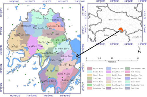
The study area has a subtropical monsoon climate with four distinct seasons, adequate illumination, and abundant rainfall. The annual average temperature is between 15.9°C and 16.6°C, and the annual rainfall for the total area of Janli County is between 1100 and 1300 mm in most years. The main crops grown in the study area include oil-seed rape, wheat, rice, and cotton. Among these crops, oil-seed rape and wheat are harvested in summer and called summer-harvest crops, and rice and cotton are harvested in autumn and called autumn-harvest crops.
2.2. HJ-1 CCD data
The HJ-1 CCD is one of the key instruments carried by the HJ-1 satellite constellation and has been used in regional and global applications in agriculture, environment, and land surveys (Zhong et al. Citation2014). The HJ-1 satellite constellation consists of three satellites: HJ-1A, HJ-1B, and HJ-1C. HJ-1A and HJ-1B have two CCD cameras each. These four CCD cameras work simultaneously to make a swath of about 700 km wide with a revisit period of four days and reach a two-day temporal resolution when combining HJ-1A and HJ-1B. The CCD cameras take images in three visible bands (430–520 nm, 520–600 nm, and 630–690 nm) and one near-infrared band (760–900 nm) at 30-m spatial resolution (CCFRSDA Citation2014a). In our paper, the HJ-1 CCD data were selected for crop classification because HJ-1 CCD images have both relatively high spatial and high temporal resolution (30 m spatial resolution and 2-day temporal resolution).
Selected cloud-free images from the year 2013 are shown in . Nineteen images were selected, with 8 used for summer-harvest crop identification and 12 for autumn-harvest crops. The image acquired on 13 June 2013 was used for both summer-harvest and autumn-harvest crop classification.
Table 1. The dates for cloud-free images from the HJ-1 CCD.
2.3. Landsat-8 OLI data
The Landsat 8 system is the eighth American Earth observation satellite in the Landsat program. Landsat 8 OLI has a spatial resolution of 30 m for multi-spectral bands and 15 m for the panchromatic band 8, with a revisit time of 16 days. In our study, the Landsat 8 OLI image (path 123 and row 39) from 31 July 2013 was selected for masking non-vegetation areas using its pan-sharpened multi-spectral bands, as it has similar spectral characteristics with the HJ-1 CCD (CCFRSDA Citation2014a; USGS Citation2015). The specific comparisons between Landsat 8 OLI imagery and HJ-1 CCD are listed in . We used the panchromatic band 8 at 15 m resolution, and increased the spatial resolution of the multi-spectral bands (bands 1–7) from 30 m to 15 m by applying the pan-sharpening technique (Johnson, Scheyvens, and Shivakoti Citation2014). Although the 16-day temporal resolution limits the retrieval of crop biophysical parameters that are rapidly changing during the season, 15 m pan-sharpened Landsat 8 image is more appropriate for smaller non-vegetation surface features for comparisons with 30 m HJ-1 CCD images. Therefore, the Landsat 8 image in July was used for discriminating vegetation areas from non-vegetation areas.
2.4. Validation data
ZiYuan (ZY)-3 satellite images were selected as the validation images due to their higher spatial resolution (5.8 m) than the HJ-1CCD imagery. The ZY-3, a Chinese Earth observation satellite, was launched in January 2012 (CCFRSDA Citation2014b). The swath width of the multi-spectral camera on the ZY-3 is 51 km, and the swath width of the HJ-1 CCD is 700 km. Specific comparisons between multi-spectral camera of ZY-3 and HJ-1 CCD are listed in and . In this study, a ZY-3 image (path 2 and row 149) from 6 April 2013 was selected for validating the wheat and rape map, and an image (path 4 and row 150) from 28 July 2013 for the cotton map.
Table 2. Landsat 8 OLI and HJ-1 CCD.
Table 3. ZY-3 satellite.
The statistical data about the planted area for each crop in Jianli County except two-season rice were collected from the Jingzhou Statistical Yearbook for validation (Hu Citation2014).
2.5. Data processing
All these satellite images were further pre-processed using the remote sensing software ENVI (Zhong et al. Citation2014). This pre-processing included geometric correction, radiometric calibration, atmospheric correction, georeferencing, and pan-sharpening. Landsat 8 imagery was used as a reference image for the geometric correction of HJ-1 CCD and ZY-3 data. We conducted radiometric calibration and atmospheric correction for Landsat 8, ZY-3 and HJ-1 CCD images using the Fast Line-of-Sight Atmospheric Analysis of Spectral Hypercubes (FLAASH) algorithm. The HJ-1 CCD and ZY-3 images were corrected with the image-to-image registration mode and all images were projected to the UTM map projection, WGS 84 Zone 49 North. To improve the spatial resolution of Landsat 8 imagery, we applied a pan-sharpening process using the Gram-Schmidt Pan-Sharpening method integrated in ENVI. The resampling method was cubic convolution during the process of image fusion. Gram-Schmidt is typically more accurate than other methods because it uses the spectral response function of a given sensor to estimate what the panchromatic data should look like. Image pan-sharpening increased the spatial resolution of the multi-spectral Landsat 8 image bands from 30 m to 15 m, using the spatial information in15 m pan band.
2.6. Field survey data
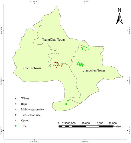
Field survey data were collected from five growing seasons. Thirty GPS sampling points for crops were collected within the county, including three for maize, nine for oil-seed rape, nine for middle-season rice, two for seasonal rice, five for cotton, and two for grass and trees. The spatial distribution of the 30 GPS points is shown in .
Figure 2. GPS points for field survey.
The phenological calendars were collected in 2010, 2011, 2012, 2013, 2014 and 2015. – show the phenological calendars for wheat, rape, two-season rice (early season rice and late rice), middle-season rice and cotton. In these tables, the date is the ending date of the corresponding growth stage, and the duration is the number of days in the growth stage. The date and duration are the average of field survey data collected over a five-year period.
Table 4. Phenological calendars of wheat and rape.
Table 5. Phenological calendars of two-season rice.
Table 6. Phenological calendars of wheat and rape.
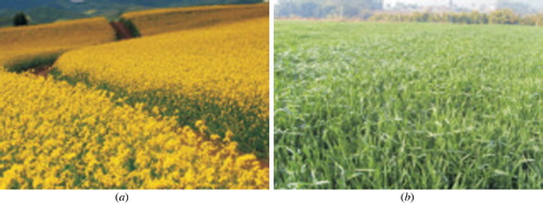
shows field photos of wheat and oil-seed rape taken in the study area. From these photos, oil-seed rape in the full blooming phase on the left had a yellow colour on 25 March 2013, but the wheat in the booting phase on the right has a green colour on 3 April 2013. During the five-year survey period, oil-seed rape and wheat show this difference every year.
Figure 3. Photos for oil-seed rape and wheat through field observation: (a) The field photo for oil-seed rape taken on 25 March 2013; (b) The field photo for wheat taken on 3 April 2013.
3. Method
3.1. Masking non-vegetation areas
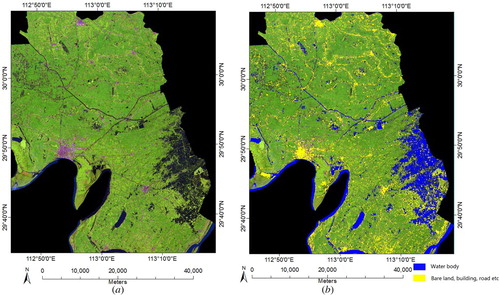
Agricultural vegetation areas are the focus for the study, so non-vegetation areas should be eliminated using a mask and applying a vegetation mask prior to crop classification reduces confusion between crop types and surrounding surface features. Before mapping the crop planting structure therefore, we masked out the non-vegetation land cover of water, fishponds, bare land, buildings, and roads using Landsat 8 imagery. We acquired the Landsat 8 imagery for the growing season (31 July 2013) and set different display colours for vegetation and non-vegetation areas in the composite image of bands 6, 5, and 2, e.g. water appears as black and bare land as pink ((a)). This distinction helps us to identify non-vegetation from crops. We applied the minimum distance method of supervised classification, with the help of visual interpretation methods, to the Landsat 8 image. The non-vegetation types were acquired and used as a mask layer to select vegetation areas from the study area. (b) shows the masking layer results obtained by supervised classification. In the masking layer, blue represents bodies of water and yellow represents bare land, buildings, roads, etc.
Figure 4. Masking non-vegetation areas: (a) False colour image composed from bands 6, 5, and 2; (b) the results of masking non-vegetation areas.
3.2. Extracting key phenological metrics from time-series NDVI
3.2.1. Definition of four key phenological metrics
Crop classification was conducted on the crop area masked by non-vegetation areas. The discriminating factors include the seasonal change rule (temporal characteristics of NDVI value in crop growth cycles) and spectral characteristics of different crops.
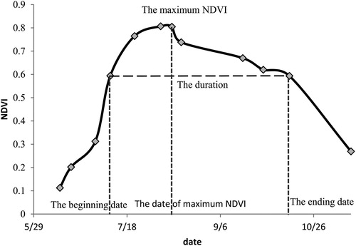
NDVI is one of most common indicators used to detect the seasonal change of vegetation over large areas. As an indicator of temporal signals, NDVI may be used to derive key phenological metrics, e.g. start of growing season, length and end of season, or peak of leaf area index (Tang Citation2015). In this study, four key phenological metrics were extracted from time-series NDVI curves to show the change of NDVI values during crop growth (). The threshold value, 0.6, was determined by statistical investigation at a known area in Jianli County using the ZY-3 satellite image.
Duration: the number of days when NDVI is greater than 0.6; if the duration occurs more than once, the largest number of days is selected.
Beginning date: the start date when NDVI is greater than 0.6, corresponding to the jointing stage of crops.
Ending date: the date of the final stage when NDVI is greater than 0.6, corresponding to the end of the pustulation period.
Date of maximum NDVI: The date of maximum NDVI in the growth period, corresponding to the ending stage of crop vegetative growth or the earlier stage of crop reproductive growth.
Figure 5. Four phenological metrics that show the change in NDVI values during middle-season rice growth.
3.2.2. Main crop time-series NDVI curves for Jianli County
After pre-processing all the selected cloud-free HJ-1 CCD images, these time-series HJ-1/CCD data were used to construct time-series NDVI curves. Thirty GPS sampling points for crops were collected within the county to acquire the typical NDVI curve of the main crops in Jianli. Every point, as a pure pixel, represents a specific crop with a large area. NDVI values in the same site with GPS points were extracted from the corresponding HJ-1 CCD images. Finally, the constructed time-series NDVI curves for summer-harvest crops and autumn-harvest crops are shown in and , respectively.
Figure 6. Time-series NDVI curves for summer-harvest crops from January to June.
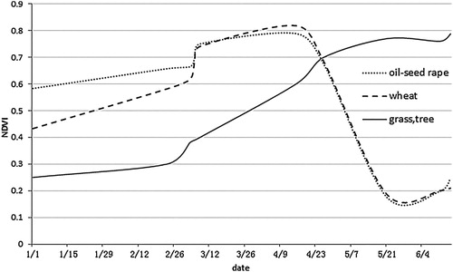
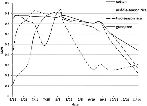
Figure 7. Time-series NDVI curves for autumn-harvest crops from June to November.
3.2.3. Key phenological metrics of crops extracted from time-series NDVI curves
3.2.3.1. Summer-harvest crops
Flourishing oil-seed rape and wheat usually has relatively high NDVI and LAI values during March and April (Sun, Cao, and Huang Citation2009; Zhao et al. Citation2013). After May, these two crops step into the late growth stage and chlorophyll content descends, causing lower NDVI values. However, from March to June, the chlorophyll content of grass and trees descends, causing their NDVI values to also decrease ( and ). As shown in , phenological metrics can be used to identify grass and trees from crops; however, rapeseed and wheat still have similar phenological metrics and a further classification is needed, which we will discuss in Section 3.3.
Table 7. Phenological metrics from time-series NDVI curves.
3.2.3.2. Autumn-harvest crops
The difference in phenological metrics between autumn-harvest crops (middle-season rice, two-season rice and cotton) and non-crop vegetation (grass and trees) are extracted from the time-series NDVI curves ( and ). Different from summer-harvest crops, the autumn-harvest crops have a later starting date and shorter duration than the grass and trees, as well as more fluctuation among crops.
3.3. Crop classification
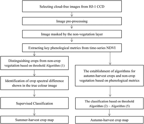
Cloud-free images were selected from HJ-1 data, and the time-series NDVI curve was created before crop classification. The non-vegetation was removed but all vegetation including crop and non-crop vegetation was kept since July is in the growing season. Key phenological metrics were extracted from time-series NDVI, and then crop classification was conducted based on those phenological metrics. shows the detailed flowchart of crop classification for both summer-harvest (mainly oil-seed rape and wheat) and autumn-harvest crops (mainly rice and cotton). In the following paragraphs, we will introduce the crop classification method seen in using an algorithm based on phenological metrics in which the thresholds are acquired from field survey and time-series NDVI curves for the study area.
Figure 8. Flow chart of crop classification for summer-harvest crops and autumn-harvest crops.
3.3.1. Summer-harvest crop classification
The oil-seed rape and wheat areas are first distinguished from trees and grass according to key phenological metrics shown in Section 3.2. Based on field investigation and key phenological metrics extracted from NDVI curves, we designed the threshold classification algorithm between summer-harvest crops and non-crops as:
If NDVIgrow > 0.4 and NDVIharvest < 0.2, then oil-seed rape and wheat (1)
In this algorithm, four dates (4 March, 6 March, 15 April, and 26 April) were selected as the growing period to represent NDVIgrow, and two dates (13 May and 13 June) represent the harvest period NDVIharvest. Then an IDL (Interactive Data Language) program in ENVI software was coded according to the classification algorithm (Algorithm (1)) to distinguish oil-seed rape and wheat from trees and grass, and finally we get the crop vegetation areas only including oil-seed and wheat crops.
After that, we distinguished oil-seed rape from wheat. In , the NDVI time-series curves and key phenological metrics are similar between oil-seed rape and wheat; therefore, it is hard to identify these two crops only according to phenological metrics. In this study, we classified them according to spectral characteristics in HJ-1 CCD images on 6 March 2013, and 15 April 2013. Based on the spectral characteristics of wheat and oil-seed rape in bands 3, 2, and 1, we performed a minimum distance classification using HJ-1 CCD data from the beginning of March to the beginning of April. According to five years of field surveys in the study area (), the spectral characteristics between wheat and oil-seed rape during the flowering phase of oil-seed rape are different. The reflectance value of oil-seed rape increases during the flowering phase at bands 2 (spectral range 520–600) and 3 (spectral range 630–690) due to increasing reflectance in the spectrum at 500–700 nm. Meanwhile, the reflectance value of wheat in the spectral range of 520–600 nm is high during this phrase. Therefore, in the true colour image composited from bands 3, 2, and 1, the oil-seed rape in the flowering phase shows a yellow colour, but the wheat still shows a green colour during this period. We selected yellow areas as the training samples of oil-seed rape and green areas as the training samples of wheat from the true colour image, and then applied the supervised classification method (minimum distance) to classify these two crops and extract their spatial distribution in the study area.
3.3.2. Autumn-harvest crop classification
Unlike with the summer-harvest crops, the key phenological metrics among middle-season rice, two-season rice, and cotton are different from each other as well as from trees and grass ( and ). Therefore, we applied the similar threshold method to classify the autumn-harvest crops and non-crop vegetation. The threshold classification algorithm is designed based on field investigations and four key phenological metrics ( and ):
If 100 days < Duration < 140 days, Datebeginning = mid-June and Dateending = early October, then non-crops (Grass and Trees) (2)
If 70 days < Duration < 110 days, Datebeginning = late June, Dateending = late August, and DatemaxiNDVI = mid-July, then middle season rice (3)
If 60 days < Duration < 80 days, Datebeginning = late July, Dateending = early October, and DatemaxiNDVI = mid-August, then two-season rice (4)
If 70 days < Duration < 100 days, Datebeginning = mid-July, Dateending = mid-October, and DatemaxiNDVI = early August, then cotton (5)
In these algorithms, Duration refers to the number of days when NDVI is greater than 0.6 (corresponding to the first key phenological metric in Section 3.2.1); Datebeginning is the start date when NDVI is greater than 0.6 (corresponding to the second key phenological metric in Section 3.2.1); Dateending is the date of the final stage when NDVI is greater than 0.6 (corresponding to the third key phenological metric in Section 3.2.1); DatemaxiNDVI is the date of maximum NDVI in the growth period (corresponding to the fourth key phenological metric in Section 3.2.1).
Finally, to classify middle-season rice, two-season rice, cotton, and non-crops, the IDL program for the threshold classification algorithm in ENVI was coded according to the above algorithms (from algorithm (2) to algorithm (5)) to get the middle-season rice, two-season rice, and cotton area.
3.4. Validation method
In this study, we compared the summer-harvest crop results with results derived from ZY-3 satellite images by using the Kappa coefficient K. The autumn-harvest crop results were compared with results derived from ZY-3 satellite images by using the Kappa coefficient and the correlation coefficient R.
The kappa coefficient measures the agreement between the classification and truth values (the classification results from ZY-3 were considered the ‘truth’ values in this study) (Cohen Citation1960). The kappa coefficient (K) is calculated as:(1) In Equation (1), i is the class number; N is the total number of classified values compared with truth values; Xi,i is the number of values belonging to the truth class i that have also been classified as class i (i.e. values found along the diagonal of the confusion matrix); Gi is the total number of truth values belonging to class i; and Hi is the total number of classification values belonging to class i.
The correlation coefficient R measures the agreement between the autumn-harvest crop inversion areas and actual value for villages or towns (the actual value was from ZY-3 data in this study). The calculation method of correlation coefficient R is based on the method of the Pearson product–moment correlation coefficient (Pearson Citation1895):(2) In Equation (2), I is the class number; n is the total number of inversion values compared with actual values; xi is the number of inversion values belonging to class i; yi is the number of actual values belonging to class I;
is the mean value of n numbers xi; and
is the mean value of n numbers yi.
4. Results and discussion
4.1. Crop mapping results
4.1.1. Summer-harvest crop classification results
(a) shows the classification result of crop vegetation from phenological metrics in the spring of 2013. The final oil-seed rape and wheat classification results are seen in (b) and the crop area for villages and towns are listed in . These results suggest that the sum of the planting areas for oil-seed rape and wheat is about 1178.34 km2. The oil-seed rape area is much larger than wheat, and total oil-seed rape area within Jianli County is up to 1038.07 km2.
Figure 9. The classification results for summer-harvest crops: (a) crop vegetation map; (b) summer-harvest crop map.
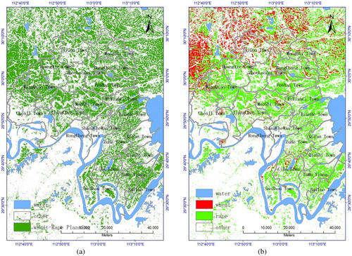
Table 8. Summer-harvest crop areas for villages or towns (unit: km2).
4.1.2. Autumn-harvest crop classification results
The final autumn-harvest map is shown in and the crop area for each village and town is listed in . The total area of middle-season rice is 893.40 km2, planted in Jiangcheng, Zhoulao and Huangxie; the total area of two-season rice is 42.67 km2, planted in Huangxie and Chengji; and the area of cotton is 236.40 km2, in Chengji.
Figure 10. Autumn-harvest crop map.
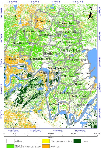
Table 9. Autumn-harvest crop areas for villages or towns (unit: km2).
4.2. Validation and discussion
4.2.1. Accuracy assessment using ZY-3
ZY-3 images were classified by using supervised classification based on the minimum distance method .The resulting maps were used to validate the data. For the ZY-3 image on 6 April 2013, the sampling method was the same as the summer-harvest classification scheme discussed in Section 3.3.1. We selected yellow areas as the training samples for oil-seed rape and green areas as the training samples for wheat, from the true colour ZY-3 image, and extracted the spatial distribution of rape and wheat for map validation. During the whole growth stage of autumn-harvest crops, only the ZY-3 image on 28 July 2013 was acquired. The cotton on this date shows a dark green colour, and is different from other surface features, but rice has a colour similar to surrounding vegetation. Therefore, we selected dark green areas as the training samples for cotton from the true colour image of ZY-3 and extracted the spatial distribution of cotton for cotton map validation. The crops mapping results from ZY-3 images are not validated by field survey, but ZY-3 images have better legibility and recognition on agriculture areas given their high spatial resolution and good radiometric quality (Lin et al. Citation2013). Therefore, the classification results from 5.8 m ZY-3 images are reliable and more accurate than 30 m HJ-1 CCD images.
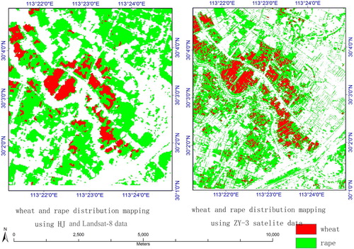
shows a comparison of summer-harvest map results for the HJ-1 CCD and ZY-3 images. The Kappa coefficient calculated using Equation (1) introduced in Section 3.4 is 0.94, between our classification results and results derived from ZY-3 satellite images, which was considered the true spatial distribution of summer-harvest crops. The summer-harvest map results show that our method is feasible for classifying oil-seed rape and wheat.
Figure 11. Comparison of summer-harvest crop classification.
presents a comparison of cotton distribution from the HJ-1 CCD and ZY-3, and the cotton distribution areas for the villages or towns are shown in . The Kappa coefficient between the cotton classification results and results derived from ZY-3 satellite images is 0.90. From , it can be inferred that the spatial distribution of cotton from the HJ-1 CCD was consistent with that derived from ZY-3 images. From , the correlation coefficient R between the inversion value and actual value calculated using Equation (2) introduced in Section 3.4 is 0.96, which means that the map results are close to the real crop maps and that our approach for the classification of the autumn-harvest crop is practical.
Figure 12. Comparison of cotton distribution maps.
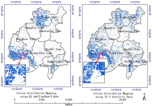
Table 10. Comparison of cotton areas for villages or towns (unit: km2).
4.2.2. Analysis of accuracies from statistical data
represents a comparison between the size of crop area extracted from and and the statistical data from the Jingzhou Statistical Yearbook. The statistical data do not include two-season rice data (). From , the inversion values of middle-season rice, cotton, oil-seed rape, and wheat agree with the statistical data with an average precision of about 72.5% (average values of 85%, 70%, 65%, and 70%, respectively).
Table 11. Classification accuracy assessment using statistical data.
Since the mapping method is based on two sources of satellite images, the classification accuracy depends on the precision of geometric correction among the different satellite images. The error in geometric correction cannot exceed one pixel; otherwise, the classification accuracy will be seriously affected. The overall classification accuracy is 72.5%. There are three things that affect the classification. First, agricultural statistical data are often updated by communication with farmers or land surveys to identify crop types (Peña-Barragán et al. Citation2011). The statistical information collected by government agencies tends to be limited in spatial coverage and crop categories, so data accuracy cannot be guaranteed (Zhong Citation2012). Second, the heterogeneous landscapes where individual fields are located are often smaller than the one-pixel areas collected from satellite images. This inconsistency reduces classification accuracy (Fritz et al. Citation2008; Löw and Duveiller Citation2014). Moreover, the classification error for crops with low phenological discrepancy such as wheat and oil-seed rape is greater than those with high phenological discrepancy such as middle-season rice.
4.2.3. Discussion
It is very difficult to find remote sensing data at both high spatial resolution and high temporal frequency. Middle to high spatial resolution satellite data, for example, data from the Landsat, SPOT, and Indian Remote Sensing satellites, might capture croplands with small-sized fields, but the data with high cost and low temporal frequency counteract their spatial resolution advantages (Wu and Li Citation2012; Wang et al. Citation2016). HJ-1 CCD images, however, provide a new type of free open source data with high spatial and temporal resolution, and have substantially increased the availability of regional cloud-free optical remote sensing data (Zhong, Gong and Biging Citation2014). One study demonstrated that continuous rice growth monitoring over time and space at the field level can be implemented effectively with HJ-1 CCD data (Wang et al. Citation2016), while another study identified paddy rice in Yuanjiang City using time-series HJ-1 CCD imagery (Zhao et al. Citation2016). Similarly, our study also demonstrates the potential of phenological metrics-based crop classification using HJ-1 CCD images. However, HJ-1 CCD data mostly cover China and some surrounding Asian countries and not the whole globe, and the sensors only have four wavebands (Wang et al. Citation2016). Therefore, in the future, we will explore the potential of SAR such as Sentinel-1 and optical remote sensing data such as Gaofen series satellite for regional crop classification.
In this study, we extracted a crop map according to phenological metrics from HJ-1 CCD images after masking the non-vegetation areas from Landsat 8 imagery. This approach is different from studies that used single multi-temporal satellite data, identified crop/non-crop, irrigated/non-irrigated croplands, or only identified one specific crop such as rice (Wardlow, Egbert, and Kastens Citation2007; Zhang et al. Citation2011; Manjunath et al. Citation2015; Lee, Kastens, and Egbert Citation2016). Other studies focused on enhanced time-series data using multi-sensor satellite images (Hao et al. Citation2014; Li et al. Citation2015). We identified crop types not by using a one-step classification but through a sequential masking approach. In our future work, we will apply this method to more study areas and further improve the technique.
The field survey data in our research are limited as obtaining reliable and accurate field data at an appropriate scale are a challenging endeavour (Fisher and Mustard Citation2007); however, the phenology-based classification approach has advantages when the availability of ground-truth data is limited (Zhong et al. Citation2011). Sampling points in our study were selected specifically for the phenological period collection. Each field sample is corresponding to a single crop type with large area, and is the representative of different crops found in Jianli County. Moreover, these sampling points are centrally distributed in three towns as they are the permitted collection of field survey data. In the future, the suitable threshold acquired from these field data will be used and validated in other districts.
Our work also presents an example of crop identification through the phenological metrics extracted from crop NDVI time-series curves using HJ-1 CCD images. Crop mapping in our study area was established on the phenological discrepancy among crops. Phenological metrics of different crops are the temporal characteristics that indicate crop seasonality (Zhong et al. Citation2011). Phenological metrics from multi-temporal satellite images have the potential to indicate crop growth development in a large region (Fisher and Mustard Citation2007; Zhong et al. Citation2011; Zhong, Gong and Biging Citation2014; Li et al. Citation2014). The study region of our paper is very small. However, Jianli County is the typical and representative area of Sihu plain-lake district in central and southern Hubei province, and an important base of agricultural production. It is the renowned ‘country of fish and rice’ in China. In the future, we will apply this method to the Sihu plain-lake district with an area of 11,547 km2 to further validate this approach.
5. Conclusions
In China, farmlands with small parcel sizes, diversified crops, and cloudy weather limit accurate discrimination of crop by remote sensing data. We provide an easy and quick method to mask non-vegetation areas by visual interpretation combined with the supervised classification results from Landsat 8 images. Four key phenological metrics are defined and derived to represent the seasonal characteristics found in NDVI time-series curves. These four phenological metrics were successfully extracted from multi-temporal NDVI time-series images, and the spatial distribution of the main crops planted in Jianli County was acquired by a feature extraction method. The cost of the entire programming procedure was contained at a low level. In the future, we will define the threshold automatically and enable automatic operation in the extraction of crop spatial distributions using HJ-1 CCD images.
Our results show that the classification accuracy of summer-harvest and autumn-harvest crops is favourable through a comparison with the classification results using ZY-3 data and related statistical records. Therefore, the crop classification technique described here represents a valuable exploration in the field of crop classification.
Although the method in the study is quick and easy, the trees, grass, and other non-crops may be omitted and should be identified again. In the future, the accuracy of crop mapping needs to be improved. Moreover, the classification method in the study should be applied to other vegetation or land use types.
Acknowledgements
We are grateful to the anonymous reviewers for their valuable comments, and also acknowledge informative and helpful discussions with Stephen McClure of George Mason University.
Disclosure statement
No potential conflict of interest was reported by the authors.
Additional information
Funding
References
- Becker-Reshef, I., C. Justice, M. Sullivan, E. Vermote, C. Tucker, A. Anyamba, J. Small, E. Pak, E. Masuoka, and J. Schmaltz. 2010. “Monitoring Global Croplands with Coarse Resolution Earth Observations: The Global Agriculture Monitoring GLAM Project.” Remote Sensing 2: 1589–1609. doi: 10.3390/rs2061589
- Blaes, X., L. Vanhalle, and P. Defourny. 2005. “Efficiency of Crop Identification Based on Optical and SAR Image Time Series.” Remote Sensing of Environment 96 (3): 352–365. doi: 10.1016/j.rse.2005.03.010
- Boryan, C., Z. Yang, R. Mueller, and M. Craig. 2011. “Monitoring US Agriculture: The US Department of Agriculture, National Agricultural Statistics Service, Cropland Data Layer Program.” Geocarto International 26 (5): 341–358. doi: 10.1080/10106049.2011.562309
- CCFRSDA (China Centre For Resource Satellite Data and Application). 2014a. “HJ-1 CCD Webpage.” http://www.cresda.com/CN/Satellite/3064.shtml
- CCFRSDA (China Centre For Resource Satellite Data and Application). 2014b. “ZY-3 Webpage.” http://www.cresda.com/CN/Satellite/3070.shtml
- Cohen, J. 1960. “A Coefficient of Agreement for Nominal Scales.” Educational and Psychological Measurement 20: 37–46. doi: 10.1177/001316446002000104
- Crapper, P. 1980. “Errors Incurred in Estimating an Area of Uniform Land Cover Using Landsat.” Photogrammetric Engineering and Remote Sensing 46 (10): 1295–1301.
- Crook, F. W. 1993. “Underreporting of China’s Cultivated Land Area: Implications for World Agricultural Trade.” US Department of Agriculture, China International Agricultural and Trade Rep. No. RS-93-4, Washington, DC, USA. Situation and Outlook Series, 33–39.
- Dong, J., X. Xiao, W. Kou, Y. Qin, G. Zhang, L. Li, C. Jin, Y. Zhou, J. Wang, and C. Biradar. 2015. “Tracking the Dynamics of Paddy Rice Planting Area in 1986–2010 Through Time-series Landsat Images and Phenology-based Algorithms.” Remote Sensing of Environment 160: 99–113. doi: 10.1016/j.rse.2015.01.004
- Doraiswamy, P. C., T. R. Sinclair, S. Hollinger, B. Akhmedov, A. Stern, and J. Prueger. 2005. “Application of MODIS Derived Parameters for Regional Crop Yield Assessment.” Remote Sensing of Environment 97 (2): 192–202. doi: 10.1016/j.rse.2005.03.015
- FAO. 1995. Programme for the World Census of Agriculture 2000 (WCA 2000). Statistical development series 5. Rome: Food and Agriculture Organization of the United Nations.
- Fisher, J. I., and J. F. Mustard. 2007. “Cross-scalar Satellite Phenology from Ground, Landsat, and MODIS Data.” Remote Sensing of Environment 109 (3): 261–273. doi: 10.1016/j.rse.2007.01.004
- Forkuor, G., C. Conrad, M. Thiel, T. Landmann, and B. Barry. 2015. “Evaluating the Sequential Masking Classification Approach for Improving Crop Discrimination in the Sudanian Savanna of West Africa.” Computers and Electronics in Agriculture 118: 380–389. doi: 10.1016/j.compag.2015.09.020
- Forkuor, G., C. Conrad, M. Thiel, T. Ullmann, and E. Zoungrana. 2014. “Integration of Optical and Synthetic Aperture Radar Imagery for Improving Crop Mapping in Northwestern Benin, West Africa.” Remote Sensing 6 (7): 6472–6499. doi: 10.3390/rs6076472
- Fritz, S., M. Massart, I. Savin, J. Gallego, and F. Rembold. 2008. “The Use of MODIS Data to Derive Acreage Estimations for Larger Fields: A Case Study in the South-western Rostov Region of Russia.” International Journal of Applied Earth Observation and Geoinformation 10 (4): 453–466. doi: 10.1016/j.jag.2007.12.004
- Gumma, M. K., P. S. Thenkabail, P. Teluguntla, M. N. Rao, I. A. Mohammed, and A. M. Whitbread. 2016. “Mapping Rice-fallow Cropland Areas for Short-season Grain Legumes Intensification in South Asia Using MODIS 250 m Time-series Data.” International Journal of Digital Earth 9 (10): 981–1003. doi: 10.1080/17538947.2016.1168489
- Hao, P., L. Wang, and Z. Niu. 2015. “Potential of Multitemporal Gaofen-1 Panchromatic/Multispectral Images for Crop Classification: Case Study in Xinjiang Uygur Autonomous Region, China.” Journal of Applied Remote Sensing 9 (1): 096035–096035. doi: 10.1117/1.JRS.9.096035
- Hao, P., L. Wang, Z. Niu, A. Aablikim, N. Huang, S. Xu, and F. Chen. 2014. “The Potential of Time Series Merged from Landsat-5 TM and HJ-1 CCD for Crop Classification: A Case Study for Bole and Manas Counties in Xinjiang, China.” Remote Sensing 6 (8): 7610–7631. doi: 10.3390/rs6087610
- Hu, J. 2014. Jingzhou Statistical Yearbook. Beijing: China Statistics.
- Jia, K., B. Wu, and Q. Li. 2013. “Crop Classification Using HJ Satellite Multispectral Data in the North China Plain.” Journal of Applied Remote Sensing 7 (1): 073576–073576. doi: 10.1117/1.JRS.7.073576
- Johnson, B. A., H. Scheyvens, and B. R. Shivakoti. 2014. “An Ensemble Pansharpening Approach for Finer-Scale Mapping of Sugarcane with Landsat 8 Imagery.” International Journal of Applied Earth Observation and Geoinformation 33 (12): 218–225. doi: 10.1016/j.jag.2014.06.003
- Kumar, P., R. Prasad, A. Choudhary, V. N. Mishra, D. K. Gupta, and P. K. Srivastava. 2017. “A Statistical Significance of Differences in Classification Accuracy of Crop Types Using Different Classification Algorithms.” Geocarto International 32 (2): 206–224.
- Lee, E., J. H. Kastens, and S. L. Egbert. 2016. “Investigating Collection 4 Versus Collection 5 MODIS 250 m NDVI Time-series Data for Crop Separability in Kansas, USA.” International Journal of Remote Sensing 37 (2): 341–355. doi: 10.1080/01431161.2015.1125556
- Li, Q., X. Cao, K. Jia, M. Zhang, and Q. Dong. 2014. “Crop Type Identification by Integration of High-spatial Resolution Multispectral Data with Features Extracted from Coarse-resolution Time-series Vegetation Index Data.” International Journal of Remote Sensing 35 (16): 6076–6088. doi: 10.1080/01431161.2014.943325
- Li, Q., C. Wang, B. Zhang, and L. Lu. 2015. “Object-based Crop Classification with Landsat-MODIS Enhanced Time-series Data.” Remote Sensing 7 (12): 16091–16107. doi: 10.3390/rs71215820
- Lin, L., H. Luo, H. Zhu, Z. Li, and X. Tang. 2013. “User-oriented Image Quality Assessment of ZY-3 Product in Agriculture Area.” International Conference on Agro-Geoinformatics IEEE 59:22–27.
- Liu, M. W., M. Ozdogan, and X. Zhu. 2014. “Crop Type Classification by Simultaneous Use of Satellite Images of Different Resolutions.” IEEE Transactions on Geoscience and Remote Sensing 52 (6): 3637–3649. doi: 10.1109/TGRS.2013.2274431
- Löw, F., and G. Duveiller. 2014. “Defining the Spatial Resolution Requirements for Crop Identification Using Optical Remote Sensing.” Remote Sensing 6 (9): 9034–9063. doi: 10.3390/rs6099034
- Manjunath, K., R. S. More, N. Jain, S. Panigrahy, and J. Parihar. 2015. “Mapping of Rice-cropping Pattern and Cultural Type Using Remote-sensing and Ancillary Data: A Case Study for South and Southeast Asian Countries.” International Journal of Remote Sensing 36 (24): 6008–6030. doi: 10.1080/01431161.2015.1110259
- McNairn, H., C. Champagne, J. Shang, D. Holmstrom, and G. Reichert. 2009. “Integration of Optical and Synthetic Aperture Radar (SAR) Imagery for Delivering Operational Annual Crop Inventories.” ISPRS Journal of Photogrammetry and Remote Sensing 64 (5): 434–449. doi: 10.1016/j.isprsjprs.2008.07.006
- Murakami, T., S. Ogawa, N. Ishitsuka, K. Kumagai, and G. Saito. 2001. “Crop Discrimination with Multitemporal SPOT/HRV Data in the Saga Plains, Japan.” International Journal of Remote Sensing 22 (7): 1335–1348. doi: 10.1080/01431160151144378
- Ozdogan, M. 2010. “The Spatial Distribution of Crop Types from MODIS Data: Temporal Unmixing Using Independent Component Analysis.” Remote Sensing of Environment 114 (6): 1190–1204. doi: 10.1016/j.rse.2010.01.006
- Ozdogan, M., and C. E. Woodcock. 2006. “Resolution Dependent Errors in Remote Sensing of Cultivated Areas.” Remote Sensing of Environment 103 (2): 203–217. doi: 10.1016/j.rse.2006.04.004
- Pal, M., and P. M. Mather. 2006. “Some Issues in the Classification of DAIS Hyperspectral Data.” International Journal of Remote Sensing 27 (14): 2895–2916. doi: 10.1080/01431160500185227
- Pearson, K. 1895. “Notes on Regression and Inheritance in the Case of Two Parents.” Proceedings of the Royal Society of London 58: 240–242. doi: 10.1098/rspl.1895.0041
- Peña-Barragán, J. M., M. K. Ngugi, R. E. Plant, and J. Six. 2011. “Object-based Crop Identification Using Multiple Vegetation Indices, Textural Features and Crop Phenology.” Remote Sensing of Environment 115 (6): 1301–1316. doi: 10.1016/j.rse.2011.01.009
- Simonneaux, V., B. Duchemin, D. Helson, S. Er-Raki, A. Olioso, and A. G. Chehbouni. 2008. “The Use of High-Resolution Image Time Series for Crop Classification and Evapotranspiration Estimate Over an Irrigated Area in Central Morocco.” International Journal of Remote Sensing 29 (1): 95–116. doi: 10.1080/01431160701250390
- Stehman, S., and J. A. Milliken. 2007. “Estimating the Effect of Crop Classification Error on Evapotranspiration Derived from Remote Sensing in the Lower Colorado River Basin, USA.” Remote Sensing of Environment 106 (2): 217–227. doi: 10.1016/j.rse.2006.08.007
- Sun, J., H. Cao, and Y. Huang. 2009. “Correlation Between Canopy Spectral Vegetation Index and Leaf Stomatal Conductance in Rapeseed.” Acta Agronomica Sinica 35 (6): 1131–1138. doi: 10.3724/SP.J.1006.2009.01131
- Tang, J. 2015. “Dynamic Linkages Between Vegetation Phenology and Seasonal Changes in Water Quality in the Choptank Watershed, USA.” International Journal of Remote Sensing 36: 3041–3057. doi: 10.1080/01431161.2015.1055603
- Teluguntla, P., P. S. Thenkabail, J. Xiong, M. K. Gumma, R. G. Congalton, A. Oliphant, J. Poehnelt, K. Yadav, M. Rao, and R. Massey. 2017. “Spectral Matching Techniques (SMTs) and Automated Cropland Classification Algorithms (ACCAs) for Mapping Croplands of Australia Using MODIS 250-m Time-series (2000–2015) Data.” International Journal of Digital Earth. doi:10.1080/17538947.2016.1267269.
- Upadhyay, P., A. Kumar, P. S. Roy, S. K. Ghosh, and I. Gilbert. 2012. “Effect on Specific Crop Mapping Using WorldView-2 Multispectral Add-on Bands: Soft Classification Approach.” Journal of Applied Remote Sensing 6 (1): 063524-1–063524-13. doi: 10.1117/1.JRS.6.063524
- USDA. 2004. 2002 Census of Agriculture, Volume 1, Geographic Area Series Part 51, United States – Summary and State Data. Washington, DC: US Department of Agriculture.
- US Geological Survey (USGS). 2015. “Landsat 8 Webpage.” http://landsat.usgs.gov/landsat8.php
- Wang, J., J. Huang, P. Gao, C. Wei, and L. R. Mansaray. 2016. “Dynamic Mapping of Rice Growth Parameters Using HJ-1 CCD Time Series Data.” Remote Sensing 8 (11): 931. doi: 10.3390/rs8110931
- Wardlow, B. D., and S. L. Egbert. 2008. “Large-area Crop Mapping Using Time-series MODIS 250 m NDVI Data: An Assessment for the US Central Great Plains.” Remote Sensing of Environment 112 (3): 1096–1116. doi: 10.1016/j.rse.2007.07.019
- Wardlow, B. D., S. L. Egbert, and J. H. Kastens. 2007. “Analysis of Time-series MODIS 250 m Vegetation Index Data for Crop Classification in the US Central Great Plains.” Remote Sensing of Environment 108 (3): 290–310. doi: 10.1016/j.rse.2006.11.021
- Wu, B., and Q. Li. 2012. “Crop Planting and Type Proportion Method for Crop Acreage Estimation of Complex Agricultural Landscapes.” International Journal of Applied Earth Observations and Geoinformation 16 (1): 101–112. doi: 10.1016/j.jag.2011.12.006
- Wu, B., J. Meng, Q. Li, N. Yan, X. Du, and M. Zhang. 2014. “Remote Sensing-based Global Crop Monitoring: Experiences with China’s CropWatch System.” International Journal of Digital Earth 7 (2): 113–137. doi: 10.1080/17538947.2013.821185
- Xiao, X., S. Boles, J. Liu, D. Zhuang, S. Frolking, C. Li, W. Salas, and B. Moore. 2005. “Mapping Paddy Rice Agriculture in Southern China Using Multi-temporal MODIS Images.” Remote Sensing of Environment 95 (4): 480–492. doi: 10.1016/j.rse.2004.12.009
- Xiao, X., J. Liu, D. Zhuang, S. Frolking, S. Boles, B. Xu, M. Liu, et al. 2003. “Uncertainties in Estimates of Cropland Area in China: A Comparison Between an AVHRR-derived Dataset and a Landsat TM-derived Dataset.” Global and Planetary Change 37 (3): 297–306.
- Yu, L., J. Wang, N. Clinton, Q. Xin, L. Zhong, Y. Chen, and P. Gong. 2013. “FROM-GC: 30 m Global Cropland Extent Derived Through Multisource Data Integration.” International Journal of Digital Earth 6: 521–533. doi: 10.1080/17538947.2013.822574
- Zhang, S., Y. Lei, L. Wang, H. Li, and H. Zhao. 2011. “Crop Classification Using MODIS NDVI Data Denoised by Wavelet: A Case Study in Hebei Plain, China.” Chinese Geographical Science 21 (3): 322–333. doi: 10.1007/s11769-011-0472-2
- Zhang, H., Q. Li, J. Liu, J. Shang, X. Du, L. Zhao, N. Wang, and T. Dong. 2017. “Crop Classification and Acreage Estimation in North Korea Using Phenology Features.” GIScience & Remote Sensing. doi:10.1080/15481603.2016.1276255.
- Zhang, M., Q. Zhou, Z. Chen, J. Liu, Y. Zhou, and C. Cai. 2008. “Crop Discrimination in Northern China with Double Cropping Systems Using Fourier Analysis of Time-series MODIS Data.” International Journal of Applied Earth Observation and Geoinformation 10 (4): 476–485. doi: 10.1016/j.jag.2007.11.002
- Zhao, J., W. Huang, Y. Zhang, and Y. Jing. 2013. “Inversion of Leaf Area Index During Different Growth Stages in Winter Wheat.” Spectroscopy and Spectral Analysis 33 (9): 2546–2552.
- Zhao, J., C. Xu, L. Huang, D. Zhang, and D. Liang. 2016. “Characterisation of Spatial Patterns of Regional Paddy Rice with Time Series Remotely Sensed Data.” Paddy and Water Environment 14 (4): 439–449. doi: 10.1007/s10333-015-0513-z
- Zhong, L. 2012. “Efficient Crop Type Mapping Based on Remote Sensing in the Central Valley, California.” Phd diss., University of California, Berkeley.
- Zhong, L., P. Gong, and G. S. Biging. 2014. “Efficient Corn and Soybean Mapping with Temporal Extendability: A Multi-year Experiment Using Landsat Imagery.” Remote Sensing of Environment 140: 1–13. doi: 10.1016/j.rse.2013.08.023
- Zhong, L., T. Hawkins, G. Biging, and P. Gong. 2011. “A Phenology-based Approach to Map Crop Types in the San Joaquin Valley, California.” International Journal of Remote Sensing 32 (22): 7777–7804. doi: 10.1080/01431161.2010.527397
- Zhong, B., P. Ma, A. H. Nie, A. Yang, Y. J. Yao, W. B. Lu, H. Zhang, and Q. H. Liu. 2014. “Land Cover Mapping Using Time Series HJ-1/CCD Data.” Science China Earth Sciences 57: 1790–1799. doi: 10.1007/s11430-014-4877-5
- Zhong, L., L. Yu, X. Li, L. Hu, and P. Gong. 2016. “Rapid Corn and Soybean Mapping in US Corn Belt and Neighboring Areas.” Scientific Reports 6: 36240. doi: 10.1038/srep36240
- Zhou, Y., X. Xiao, Y. Qin, J. Dong, G. Zhang, W. Kou, C. Jin, J. Wang, and X. Li. 2016. “Mapping Paddy Rice Planting Area in Rice-Wetland Coexistent Areas Through Analysis of Landsat 8 OLI and MODIS Images.” International Journal of Applied Earth Observation and Geoinformation 46: 1–12. doi: 10.1016/j.jag.2015.11.001
- Zhu, S., W. Zhou, J. Zhang and G. Shuai. 2012. “Wheat Acreage Detection by Extended Support Vector Analysis with Multi-temporal Remote Sensing Images.” Proceedings of the 2012 First International Conference on Agro-geoinformatics, IEEE, Shanghai, China, August 2–4.