Global operational land imager Landsat-8 reflectance-based active fire detection algorithm

ABSTRACT

A global operational land imager (GOLI) Landsat-8 daytime active fire detection algorithm is presented. It utilizes established contextual active fire detection approaches but takes advantage of the significant increase in fire reflectance in Landsat-8 band 7 (2.20 μm) relative to band 4 (0.66 μm). The detection thresholds are fixed and based on a statistical examination of 39 million non-burning Landsat-8 pixels. Multi-temporal tests based on band 7 reflectance and relative changes in normalized difference vegetation index in the previous six months are used to reduce commissions errors. The probabilities of active fire detection for the GOLI and two recent Landsat-8 active fire detection algorithms are simulated to provide insights into their performance with respect to the fire size and temperature. The algorithms are applied to 11 Landsat-8 images that encompass a range of burning conditions and environments. Commission and omission errors are assessed by visual interpretation of detected active fire locations and by examination of the Landsat-8 images and higher spatial resolution Google Earth imagery. The GOLI algorithm has lower omission and comparable commission errors than the recent Landsat-8 active fire detection algorithms. The GOLI algorithm has demonstrable potential for global application and is suitable for implementation with other Landsat-like reflective wavelength sensors.

KEYWORDS:

• Earth observation
• remote sensing
• visible/infrared remote sensing

1. Introduction

Satellite data are used to monitor global fire activity using algorithms that detect the location of fires actively burning at the time of satellite overpass, and using burned area mapping algorithms that retrospectively map the spatial extent of the areas affected by fire. There is an established heritage for active fire detection using algorithms developed for different sensors to take advantage of the elevated radiance of fire at longer wavelengths (Matson and Dozier 1981; Robinson 1991; Prins and Menzel 1992; Giglio et al. 2003; Davies et al. 2006). Satellite active fire detections have been used in fire regime characterization studies (Schroeder et al. 2005; Giglio 2007; Loboda and Csiszar 2007; Aragão et al. 2007; Chuvieco, Giglio, and Justice 2008; Boschetti and Roy 2008), studies of human activity (FEMA 2005; Kumar et al. 2014; Pereira et al. 2015), examination of the ecological responses to fire (Lentile et al. 2006; Bowman et al. 2009), studies of active volcanism (Oppenheimer 1991), to estimate pyrogenic emissions of greenhouse gases and aerosols (Kaiser et al. 2012; Kumar et al. 2011; Zhang, Kondragunta, and Roy 2014), for wildfire fire monitoring, control, and natural resource management (Trigg and Roy 2007; Davies et al. 2009; Frost 2013), and have been used in burned area mapping algorithms (Fraser et al. 2000; Roy et al. 1999; Giglio et al. 2009; Boschetti et al. 2015). Active fire detection algorithms have predominantly been developed for high-temporal resolution satellite systems due to the ephemeral nature of fire. In particular, high-temporal but coarse spatial resolution systems with middle-infrared (3–4 μm) and thermal-infrared (10–12 μm) bands on polar-orbiting satellites, such as the advanced very high-resolution radiometer (Stroppiana, Pinnock, and Gregoire 2000) and the MODerate resolution imaging spectroradiometer (MODIS) (Giglio et al. 2003), and on geostationary satellites, such as the Meteosat second generation (Roberts and Wooster 2008) and geostationary operational environmental satellites (Prins and Menzel 1992; Zhang, Kondragunta, and Roy 2014), have been used. Active fire detection algorithms predominantly use the emitted radiance in the middle-infrared and the thermal infrared because the radiance from the coolest fires is more than two orders of magnitude greater than the radiance from a non-burning land surface in the middle-infrared and about an order of magnitude greater in the thermal infrared (Dozier 1981; Kaufman et al. 1998; Giglio et al. 2003; Wooster, Xu, and Nightingale 2012).

The Landsat satellite series offer a unique 45+ year moderate spatial resolution record of the terrestrial surface (Roy et al. 2014a). The Landsat satellites have polar circular sun-synchronous orbits and since Landsat 4 (launched 1982) acquire 30-m data with a 16-day repeat cycle. Successive temporally overlapping Landsat missions together provide eight-day full Earth coverage, although consistent coverage is not obtained because of sensor, ground station, and data communication issues and variable Landsat mission acquisition strategies (Goward et al. 2006; Wulder et al. 2016). In addition, cloud at the time of Landsat overpass may significantly reduce surface observation availability in many parts of the globe (Kovalskyy and Roy 2015). To date, the greater majority of Landsat fire research has focused on the development of burned area mapping algorithms (Boschetti et al. 2015) and for mapping the severity of fires (Cocke, Fulé, and Crouse 2005; French et al. 2008). The Landsat sensors have reflective visible to short-wave infrared bands, some sensors have thermal wavelength bands, but all lack middle-infrared bands making Landsat active fire detection challenging. The successful 2013 launch of Landsat-8 has spurned the development of Landsat-8-specific active fire detection algorithms that take advantage of the improved Landsat-8 characteristics compared to previous Landsat sensors (Schroeder et al. 2016; Murphy et al. 2016). The Landsat-8 carries the operational land imager (OLI) that has 30-m bands that are spectrally narrower than previous Landsat sensors and in particular, the OLI near-infrared (NIR) band avoids a water-absorption feature (Irons, Dwyer, and Barsi 2012). The Landsat-8 also carries the thermal infrared sensor (TIRS), although unfortunately it has stray light contamination, and so established land surface temperature retrieval algorithms are not recommended for TIRS application (Montanaro et al. 2014). Compared to previous Landsat sensors, the Landsat-8 OLI has improved calibration, signal-to-noise characteristics, higher 12-bit radiometric resolution, more precise geometry, and significantly increased global image acquisition capability (Irons, Dwyer, and Barsi 2012; Roy et al. 2014a). The moderate spatial resolution 16-day active fire detection capability provided by Landsat-8 may be useful to complement the coarser spatial but higher temporal resolution satellite active fire detection applications discussed above, particularly for detailed local scale ecological studies and natural resource management.

This paper presents a new Landsat-8 reflectance-based active fire algorithm that we refer to as the global operational land imager (GOLI) algorithm as it intended for global application. The GOLI algorithm uses fixed reflectance thresholds that were derived by statistical examination of a very large set of reflectance data and also uses the Landsat-8 band 4 (red: 0.66 μm), which is not used by recent Landsat-8 active fire detection algorithms (Schroeder et al. 2016; Murphy et al. 2016).

It is established that active fire detection omission and commission error assessment is challenging, particularly for global detection algorithms. Unlike burned areas, which have a persistent surface signal and so can be validated using higher resolution satellite data (Boschetti, Stehman, and Roy 2016), actively burning fires are ephemeral and it is not usually practical to collect a large number of ground-based measurements of fire characteristics, or even presence or absence of information, at the time of satellite overpass (Cardoso et al. 2005). Airborne remotely sensed data can be used to validate active fire detection algorithms but are expensive and difficult to coordinate (Swap et al. 2002; Schroeder et al. 2014; Peterson et al. 2013). Consequently, satellite active fire detection algorithms have been assessed by comparison of their results with simultaneously sensed remotely sensed data, notably, MODIS active fire detections have been compared with advanced spaceborne thermal emission and reflection radiometer (ASTER) data (Morisette et al. 2005a, 2005b; Csiszar, Morisette, and Giglio 2006). However, these approaches are not possible for Landsat-8 active fire detection assessment as there is no simultaneous satellite data sensed with Landsat-8, and airborne fire campaigns have not been coordinated across a range of representative conditions in the Landsat-8 era. Consequently, in this study, the probability of active fire detection is first simulated to provide insights into active fire detection omission errors using the GOLI and two recent Landsat-8 active fire detection algorithms developed by Schroeder et al. (2016) and Murphy et al. (2016). Then, the algorithm commission and omission errors are assessed by visual interpretation of detected active fire locations and by examination of the Landsat-8 images in conjunction with higher spatial resolution Google Earth imagery.

The data used are described first, followed by an examination of the Landsat-8 OLI bands suitable for active detection, and then review of previous active fire detection algorithms. The GOLI active fire detection algorithm and the Schroeder et al. (2016) and Murphy et al. (2016) algorithms are described in detail before the simulations and validation results are presented. The results and implications are discussed followed by concluding remarks.

2. Data

2.1. Landsat-8 images

Landsat-8 OLI data are available in approximately 185 km × 180 km scenes defined in a worldwide reference system (WRS-2) of path (ground track parallel) and row (latitude parallel) coordinates (Loveland and Dwyer 2012). The Landsat-8 orbital characteristics in conjunction with a 15° field of view provide a global coverage with a 16-day repeat cycle and a 10.00 a.m. equatorial over pass time (Irons, Dwyer, and Barsi 2012). The radiometric accuracy is 3% in each OLI band (Markham et al. 2014). Only the standard geolocated L1T OLI products were used in this study and have a 12-m (90% circular error) geolocation accuracy (Storey, Choate, and Lee 2014) and so are suitable for multi-temporal comparison.

Table 1 summarizes the 11 Landsat-8 images used. They encompass a diverse range of burning conditions and include images that had high (China and Indonesia-Sumatra) and low (Australia) active fire detection commission errors reported in a recent Landsat-8 active fire detection algorithm study (Schroeder et al. 2016). The US (ND) and Iraq images were chosen as they encompass gas flares that are distinct point sources that are usually considered as commission errors as they are not associated with burning vegetation. The German and Brazilian images were included as they have documented field measurements of fire size and temperature at the time of Landsat-8 overpass (Schroeder et al. 2016). Table 1 also summarizes the number of Landsat-8 images sensed in the six months prior to each image acquisition (which were used in the GOLI multi-temporal commission error reduction algorithm). Landsat can acquire the same WRS-2 path/row 22 or 23 times per year (Ju and Roy 2008) but due to complete cloud obscuration, less than 11 images were available at several of the sites in the previous six months (Table 1).

Table 1. Summary of the Landsat 8 images used in this study. All the available Landsat-8 images within the previous six months of the acquisition date were also used.

Image location	WRS-2 Path, row	Acquisition date	Number of available acquisitions in the previous six months
Australia (Northern Territory)	105, 069	08/05/2014	11
Brazil (State of Rio de Janeiro)	218, 076	19/01/2015	11
Canada (Northwest Territories)	048, 017	07/20/2014	6
China (Fujian Province)	119, 041	08/07/2014	9
Germany (Mecklenburg-Vorpommern)	194, 022	08/17/2013	8
Indonesia (Kalimantan)	118, 062	08/19/2015	11
Indonesia (Sumatra)	127, 060	06/12/2014	8
Iraq (Basrah)	166, 039	05/31/2015	11
Southern Africa (Zimbabwe and Mozambique border)	176, 072	08/06/2014	8
United States (CA)	045, 032	08/03/2014	11
United States (ND)	034, 027	07/21/2015	10

2.2. Landsat-8 pre-processing

The Landsat-8 OLI images were converted to top of atmosphere (TOA) spectral radiance (L_λ, W m⁻² sr⁻¹ μm⁻¹) and TOA spectral reflectance (ρ_λ, unitless) using the OLI L1T metadata conversion coefficients and using the scene center solar zenith angle (θ_s) stored in the metadata. Reflectance not corrected for the solar zenith angle is not intrinsic to the surface but rather changes with the position of the sun. Zhang, Roy, and Kovalskyy (2016) considered a global year of non-Antarctic Landsat-5 and Landsat-7 acquisitions and observed that the Landsat θ_s values at a given WRS-2 path/row typically varied over a year by 40° at mid-latitudes with global minimum and maximum values of 22.14° to 89.71°, respectively. We note that the TOA ρ_λ used by the Schroeder et al. (2016) active fire detection algorithm was not corrected for solar zenith angle, which will reduce the global suitability of the individual band reflectance thresholds they used. In this study, as for all Landsat-8 active detection algorithms developed to date, the Landsat data were not atmospherically corrected.

2.3. Landsat-8 active fire detection algorithm demonstration subset images

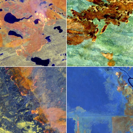
Subsets from 4 of the 11 Landsat-8 OLI L1T images were selected to illustrate the development of the active fire detection algorithm. Each subset was 300 × 300 thirty-meter pixels and included visually unambiguous actively burning fires and regions of no burning (Figure 1). The images were selected to include a likely range of fire sizes and temperatures, from high energy boreal forest fires (Canada, Northwest Territories) and mixed conifer forest fires (United States, CA), to savanna grassland fires (Southern Africa), to cooler peat fires (Indonesia, Kalimantan). Figure 1 shows false color composites of Landsat-8 bands 7 (SWIR: 2.20 μm), 6 (SWIR: 1.61 μm) and 5 (NIR: 0.87 μm) as these bands are more affected by fire (Giglio et al. 2008; Schroeder et al. 2008; Wooster, Xu, and Nightingale 2012) and are less sensitive to atmospheric contamination than the shorter wavelength visible Landsat bands (Ju et al. 2012; Roy et al. 2014b). The Indonesian subset is over peat lands (Saxon and Sheppard 2010) and so was selected to examine the active fire detection sensitivity over what is expected to be relatively cooler sub-surface smoldering fires (Siegert et al. 2004; Elvidge et al. 2015) although some surface actively burning fires are apparent.

Figure 1. Illustrative top of atmosphere Landsat-8 reflectance (2.20, 1.61, and 0.87 μm shown as red, green, and blue, respectively) for 300 × 300 thirty-meter pixel subsets of 4 images (Table 1). Top left: Canada Northwest Territories (centered on 61.7685°N, 116.5606°W), top right: Southern Africa (centered on 17.44758°S, 21.6709°E); Bottom left: US California (centered on 40.5942°N, 123.5545°W), bottom right: Indonesia Kalimantan (centered on 2.2122°S, 114.3541°E). Figures appear in color in the online version.

From each subset unambiguous actively burning fires were identified by an expert interpreter who looked for the obvious presence of active fires and fire fronts with smoke plumes. Care was taken to ensure that only fires located away from urban structures were selected for reasons that are explained later. A total of 355, 108, 256, and 77 unambiguous active fires were identified in the Canada (Northwest Territories), Southern Africa, United States (CA), and Indonesia (Kalimantan), respectively. These visually identified example active fires pixels are used to illustrate the GOLI algorithm and to examine active fire detection omission errors. In addition, 350 pixels’ locations from each image that were visually assessed as not to be burning were selected and used to model the probability of active fire detection in the subsets.

2.4. Landsat-8 non-burning reflectance data

Landsat-8 OLI spectral reflectance data used by Roy et al. (2016) to quantify differences between co-located Landsat-8 OLI and Landsat-7 Enhanced Thematic Mapper (ETM+) TOA 30-m pixel observations were used in the GOLI algorithm development. The data comprise over 59 million 30-m pixel TOA spectral reflectance values extracted systematically across the conterminous United States (CONUS) from 4272 Landsat-8 OLI images acquired over 3 summer months (28 May 2013 to 2 September 2013) and 3 Winter months (26 November 2013 to 4 March 2014). From these, only observations that were cloud-free (not labeled as high or medium confidence cloud, or as high confidence cirrus cloud) and that were not saturated were extracted. This provided 39,205,116 TOA reflectance values in each Landsat-8 reflective wavelength band that capture a broad range of land cover, land use, vegetation phenology, and soil moisture variations.

3. Active fire detection algorithm development

3.1. Initial examination of Landsat-8 reflective wavelength bands to discriminate active fires from non-burning surfaces

As illustrated in Figure 1, the Landsat-8 longer wavelength SWIR bands generally provide good active fire discrimination when the fire is unobscured by optically thick smoke. The size of actively burning fires can vary greatly, with flame fronts that can be smaller or greater than a 30-m Landsat pixel dimension (Peterson et al. 2013). Fires burn fuel in flaming and smoldering phases; the typical temperatures of smoldering and flaming fires are about 400–500 K and 800–1200 K, respectively but vary depending on factors that include the fuel characteristics and local environmental conditions (Pyne, Andrews, and Laven 1996; Kaufman et al. 1998; Giglio et al. 2008; Elvidge et al. 2015). The radiance emitted from an actively burning fire is dependent on the fire size and temperature relative to the non-burning components within the satellite observation (Kaufman et al. 1998; Giglio and Justice 2003). This is illustrated in Figure 2, which shows the Landsat-8 OLI spectral response functions (black lines) for bands 4 (0.66 μm), 5 (0.87 μm), 6 (1.61 μm), and 7 (2.20 μm), and the simulated reflectance spectra of three fires with different fire temperatures and sizes (blue, orange, and red lines) occurring on a green vegetation reflectance non-burning background (green line).

Figure 2. Simulated reflectance spectra (Equation (1)) for a flaming fire with a temperature of 1200 K covering all of the pixel (f = 1.0) (red), for a flaming fire with a temperature of 1200 K covering a small part of the pixel (f = 0.005) (orange), and cool smoldering fire with a temperature of 400 K covering all of the pixel (f = 1.0) (blue). The green line shows typical vegetation spectra (obtained from WWW1) used to define the non-burning pixel fraction. The black lines show the Landsat-8 spectral response functions for band 4 (red: 0.66 μm), band 5 (NIR: 0.87 μm), band 6 (SWIR: 1.61 μm), and band 7 (SWIR: 2.20 μm). Figures appear in color in the online version.

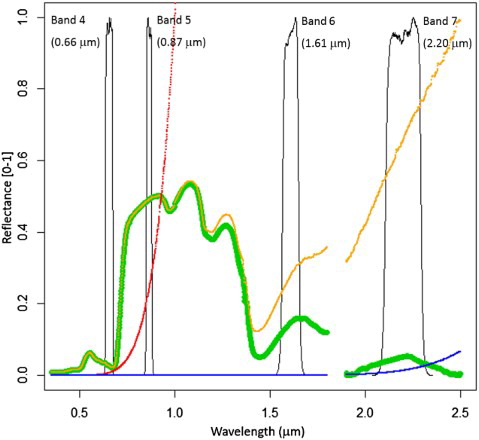
The simulated reflectance spectra illustrated in Figure 2 were derived, following (Giglio et al. 2003; Wooster, Xu, and Nightingale 2012), assuming that the active fire is an ideal black body (spectral emissivity = 1), ignoring any atmospheric contamination, and assuming that the actively burning fire had negligible reflectance, as (1) where is the simulated reflectance spectra for wavelength λ, f is the spatial fraction [0–1] of the pixel that is actively burning, is the unburned vegetation spectra, (W sr⁻¹ m⁻² m⁻¹) (defined in WWW2) is the incoming solar irradiance at the surface, and is defined as(2) where is the black body emitted radiation (W sr⁻¹ m⁻² m⁻¹), h (J s⁻¹) is the Planck constant, c (m s⁻¹) is the speed of light in a vacuum, k (J k⁻¹) is the Boltzmann constant, and T [K] is the fire temperature.

The red and orange lines in Figure 2 show the simulated reflectance spectra for a flaming fire with a temperature of 1200 K covering all of the pixel (f = 1.0) and a small fraction (f = 0.005) respectively. The blue line shows the simulated reflectance spectra for a cooler smoldering fire with a temperature of 400 K covering all of the pixel (f = 1.0). The hotter and larger fires have greater reflectance contributions in the longer wavelength bands and much less contribution in band 5 (0.87 μm), and negligible contribution in band 4 (red: 0.66 μm). The coolest 400 K fire, although it covers the whole pixel, has a very low reflectance contribution in all the illustrated reflective wavelength bands.

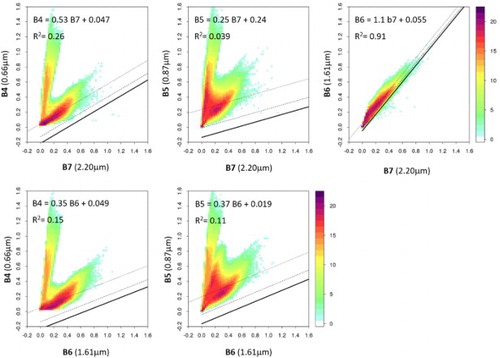
Evidently, a simple Landsat-8 active fire detection algorithm could be one that searches for high band 7 (2.20 μm) and 6 (1.61 μm) reflectance. However, the reflectance contribution of the non-burning pixel fraction may introduce commission errors. Figure 3 illustrates this, showing spectral scatterplots of the approximately 39 million CONUS TOA Landsat-8 non-burning reflectance data (Section 2.4) for different combinations of bands 4 (0.66 μm), 5 (0.87 μm), 6 (1.61 μm), and 7 (2.20 μm). The frequency of occurrence of pixels with the same reflectance value is illustrated by a 2ⁿ color scale for visual clarity. A minority of the band 4 (0.66 μm) and 5 (0.87 μm) reflectance values are greater than unity, which has been observed in other studies (Roy et al. 2014b, 2016) and is due primarily to specular reflection where the surface reflects in the satellite observation direction more strongly than a Lambertian surface (Schaepman-Strub et al. 2006). Ordinary least squares regressions of the plotted data in Figure 3 are shown by the dotted lines. All the regressions are significant with p values <.000001, but the coefficients of determination (R²) are not high due to the scatter in the reflectance values of quite different soil and vegetation types (except for the band 7 (2.20 μm) – band 6 (SWIR: 1.61 μm) scatterplot, R² = 0.91). The dashed and thick black lines show the lower 2σ and 3σ prediction intervals that describe the range of the response variable above which respectively 97.5% and 99.85% of the response variable is expected to occur, given an independent predictor variable observation. Thus, only 2.5% and 0.15% of the response values are expected to have values less than the illustrated lower 2σ and 3σ prediction intervals. The lower 2σ and 3σ prediction intervals are used in the GOLI detection algorithm. They were derived using the R statistical package and were found to be linear for the plotted data which is expected given the large sample size (Weisberg 2005).

Figure 3. Spectral scatterplots of 39,205,116 Landsat-8 OLI top of atmosphere (TOA) reflectance values extracted over land from three winter and three summer months of OLI images (4272 images) sampled systematically across the conterminous United States (Roy et al. 2016). Only observations that were cloud-free (not labeled as high or medium confidence cloud, or as high confidence cirrus cloud) and unsaturated are plotted. The frequency of occurrence of pixels with the same reflectance is illustrated by colors shaded with a 2ⁿ scale from 0 (white), 32 (blue, 2⁶ = 32), 4096 (orange, 2¹² = 4096), >1 million (purple, 2²⁰ = 1,048,576). Ordinary least squares regressions of the plotted data are shown by the dotted lines; the lower 2σ and 3σ prediction intervals are shown by the dashed and thick black lines, respectively. Figures appear in color in the online version.

3.2. Previous Landsat active fire detection algorithms

3.2.1. Overview of non-Landsat 8 algorithms

The first Landsat active fire detection algorithms were based on ones developed for ASTER active fire detection (Morisette et al. 2005a, 2005b; Giglio et al. 2008) and used thresholds derived by examination of a small number of Landsat images (Csiszar and Schroeder 2008; Schroeder et al. 2008). They identified unambiguous and potential active fire pixels using thresholds applied to the ratio and difference of SWIR and NIR reflectance in each Landsat image. Strict (high threshold) per-pixel tests were applied to identify unambiguous active fire pixels and less strict (low threshold) tests were applied to identify potential active fire pixels. The potential active fire pixel values were compared to their neighboring pixel values, using a contextual test, and only those that were significantly different were retained. It is well established that the contextual approach allows detection algorithms to be self-adaptive to local conditions and enables the detection of smaller and/or cooler fires (Prins and Menzel 1992; Flasse and Ceccato 1996; Giglio et al. 2003). In Landsat data, however, highly reflective non-burning surfaces may have high contrast with the surrounding pixels and may pass contextual tests and so be falsely labeled as active fires. In particular, this can occur for buildings, or industrial heat sources and gas flares, surrounded by less reflective vegetation (Schroeder et al. 2016). Saturation has been observed to be less prevalent in Landsat-8 reflectance data compared to previous Landsat sensors over non-burning surfaces due to the improved Landsat-8 sensor design (Roy et al. 2016). However, active fires may emit sufficient radiance to saturate Landsat-8 pixels. Landsat-8 saturation may manifest as very high or very low (including negative) reflectance (Micijevic et al. 2014; Morfitt et al. 2015).

3.2.2. Overview of Landsat-8 algorithms

Recently, two Landsat-8 OLI specific active fire detection algorithms were developed (Murphy et al. 2016; Schroeder et al. 2016). They describe nighttime and daytime algorithms, but as Landsat-8 does not operationally collect nighttime imagery, the nighttime algorithms are not considered in this study.

3.2.2.1. Murphy algorithm

The Murphy et al. (2016) Landsat-8 active fire detection algorithm is a non-contextual algorithm. Unambiguous active fires are defined as those that satisfy:(3) where ρ_λ is the TOA Landsat-8 reflectance in band λ.

Potential active fires are considered as pixels that occur next to an unambiguous active fire and satisfy:(4) where ρ_λ is the TOA Landsat-8 reflectance in band λ and Saturated ρ_λ denotes that ρ_λ is saturated. Murphy et al. (2016) did not provide tests to remove active fire detection commission errors.

3.2.2.2. Schroeder algorithm

The Schroeder et al. (2016) Landsat-8 active fire detection algorithm identifies unambiguous active fires as those that satisfy:(5) OR(6) where ρ_λ is the TOA Landsat-8 reflectance in band λ. The criteria defined by Equation (6) are intended mainly to detect fires that may be saturated.

Potential active fires are defined as those that satisfy:(7) where ρ_λ is the TOA Landsat-8 reflectance in band λ. In addition, a contextual test is applied, and only those potential active fires that satisfy the following are retained:(8) AND(9) AND(10) where ρ_λ is the TOA Landsat-8 reflectance in band λ, and σ(x) are the mean and standard deviation of x respectively in a square window centered on the potential active fire location, and max[a, b] is a function that returns the maximum value of a and b. The mean and standard deviations are computed over a 61 × 61 thirty-meter pixel window around the potential active fire pixel, ignoring unambiguous active fires defined by Equations (5) or (6) and any potential active fires defined by Equation (7), and ignoring water or shadow pixels that are defined as those satisfy the following criteria: (11)

In an attempt to deal with remaining sources of commission error, Schroeder et al. (2016) advocated a multi-temporal test. Active fire detections are labeled as ‘persistent sources’ if in the previous six months there was another active fire detected at that location and are labeled as ‘bright sources’ if the mean band 7 (2.20 μm) non-cloudy reflectance over the six months at that location was greater than 0.2.

3.3. GOLI Landsat-8 active fire detection algorithm

The above Landsat active fire detection algorithms exploit the greater increase in fire reflectance in the SWIR (band 7: 2.20 μm) relative to the NIR (band 5: 0.87 μm) to detect active fires. However, as evident in Figure 2, red reflectance (band 4: 0.66 μm) has less sensitivity to fire than NIR (band 5: 0.87 μm) reflectance. Therefore, in the GOLI algorithm, band 4 (0.66 μm) rather than band 5 (0.87 μm) is used with band 7 (2.20 μm) to detect unambiguous fires.

Unambiguous active fires are defined as those that satisfy:(12) where ρ_λ is the TOA Landsat-8 reflectance in band λ, and the two coefficients (0.53 and −0.214) are defined by the band 4 (0.66 μm) against band 7 (2.20 μm) 3σ lower prediction interval (solid line in Figure 3, top left). In Figure 3, of the 39 million pixels illustrated, only 58 pixels fall below this 3σ lower prediction interval and even if some were active fires they were found to not affect the Figure 3 regression and prediction intervals as their relative number was so small (<0.00015% of the 39 million pixels).

Pixels that are next to unambiguous active fires detected by (12) are also considered unambiguous active fires if they satisfy:(13) where ρ_λ is the TOA Landsat-8 reflectance in band λ, and the two coefficients (0.35 and −0.044) are defined by the band 4 (0.66 μm) against band 6 (1.61 μm) 3σ lower prediction interval (solid line in Figure 3, bottom left). Test (13) is implemented because hot and/or large fires may have low band 7 (2.20 μm) values due to saturation and so pass undetected by Equation (12). However, such fires are usually detected by (13) as band 6 has lower fire reflectance than band 7 (Figure 2) and is less often saturated. For these reasons, the active fire detections missed by Equation (12) but found by Equation (13) usually occur in the center of large (several pixel wide) fires.

Potential active fires are defined as those that satisfy:(14) OR(15) where ρ_λ is the TOA Landsat-8 reflectance in band λ, the two coefficients in Equation (14) are defined by the band 4 (0.66 μm) against band 7 (2.20 μm) 2σ lower prediction interval (dashed line in Figure 3, top left) which provides a less strict test than Equation (12), and the two coefficients in Equation (15) are defined by the band 6 against band 7 3σ lower prediction interval (solid line in Figure 3, top right) and provide a similar test as Equation (10) used in the Schroeder et al. (2016) potential active fire test.

The same contextual test to that used by Schroeder et al. (2016), i.e. Equations (8) and (9), is applied to the potential active fires and only those that pass the test are retained. However, the Schroeder et al. (2016) test (10) is not included as it is similar to the GOLI potential active fire test (15). In addition, a growing window dimension rather than a fixed one is used to compute the mean and standard deviation reflectance around the potential active fire detection. This is because Landsat active fire detections may occur in heterogeneous landscapes that change at scales not captured by a fixed window dimension. For example, Roy and Kumar (2017) reported that only about 5% of 1 km MODIS pixels over the Brazilian Tropical Moist Forest Biome (4 million km²) contained homogeneous land cover mapped at 30 m. The window side dimension is increased in a way similar to the approach used by the MODIS active fire contextual algorithm (Giglio et al. 2003). Specifically, the window side dimension is progressively increased from 5, 7, 9, … , to a maximum of 61 thirty-meter pixels, and the smallest dimension with at least 25% of the surrounding pixels not detected as an unambiguous or potential active fire, or as water, is used to derive the surrounding reflectance statistics. Water pixels are considered as those that satisfy the following liberal criteria that are based on the generally monotonically decreasing TOA reflectance of water bodies with wavelength (Pahlevan et al. 2014; Lymburner et al. 2016):(16) where ρ_λ is the TOA Landsat-8 reflectance in band λ.

In an attempt to deal with remaining sources of commission errors, particularly over buildings, an approach based on a refinement of the Schroeder et al. (2016) multi-temporal test is used. Active fires are rejected as commission errors if in the previous six months there was another active fire detected at that location, or if the following criteria are met:(17) OR(18) where Median_ρ2.20 is the median band 7 reflectance observed in the previous six months, is the normalized difference vegetation index (NDVI) of the active fire detection, and is the peak NDVI observed in the previous six months; NDVI denotes the normalized difference vegetation index and is defined in the conventional way as the difference in red and NIR Landsat reflectance divided by their sum. In Equation (17) the median value, rather than the mean value that was used by Schroeder et al. (2016), is implemented as it is more robust to clouds and shadows. The NDVI tests were found to help reduce commission errors over urban structures with highly reflective roofs that do not usually have as temporally variable NDVI as vegetation. Importantly, both charcoal and smoke associated with fire tend to reduce the NDVI of pixels relative to unburned equivalents (Roy et al. 1999; Fraser et al. 2000; De Moura and Galvão 2003). The thresholds in Equations (17) and (18) are set as k1 = 0.18, which is marginally lower than used by Schroeder et al. (2016), and as k2 = 0.06 which is a noise term based on Roy et al.’s (2014b) observations of the differences between the NDVI derived from Landsat TOA and surface reflectance over vegetation.

4. Results: active fire detection algorithm performance and accuracy assessment

4.1. Illustrative results

Figure 4 shows the results of applying the GOLI algorithm to the Landsat-8 subset images illustrated in Figure 1. Qualitatively, the algorithm captures active fires with detail on the spatial distribution of the fire fronts that may not be visible using coarser spatial resolution imagery. The potential GOLI active fire detections (yellow) typically occur around the periphery of the unambiguous detections (red). This is likely because fire interiors are hotter and so have higher radiance than at the periphery, and because fire periphery pixels are more likely to include cooler non-burning surfaces.

Figure 4. GOLI active fire detection results for the subsets illustrated in Figure 1. Unambiguous active fire detections are shown in red and potential active fire detections in yellow. Figures appear in color in the online version.

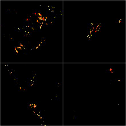
It is well established that fires can be obscured by cloud and optically thick smoke that can preclude their successful detection. However, the GOLI algorithm does not consider the cloud state when identifying active fires as fire radiance may penetrate optically thin clouds (Giglio et al. 2003) and because the Landsat-8 cloud mask is not always reliable (Kovalskyy and Roy 2015). All of the illustrated Figure 4 subsets, except the African one, were cloudy or smoke contaminated; however, the majority of the visually apparent fires were detected by the GOLI algorithm.

Figure 5 shows detailed GOLI active fire detection results extracted from images in Germany and Brazil (Table 2) that had fires at the time of Landsat-8 overpass with known location, size, and temperature (Schroeder et al. 2016). The hotter and larger German fire had a reported fire size of 11 × 13 m² with a 970-K temperature and was detected as one unambiguous active fire. The smaller and cooler Brazil fire had a reported fire size of 3 × 10 m² and cooler 870 ± 153 K temperature and was detected as two potential active fire detections. These results provide confidence in the ability of the GOLI algorithm to detect fires with areas that are a fraction of a Landsat pixel. This is investigated further below.

Figure 5. GOLI active fire detection results for 25 × 25 thirty-meter pixel subsets around the German (left: centered on 53.9276°N, 13.05870°E) and Brazilian (right: centered on 22.6868°S, 44.9844°W) sites (Table 2) that have documented fire sizes and temperatures (Schroeder et al. 2016). Top row: top of atmosphere Landsat-8 reflectance (2.20, 1.61, and 0.87 μm shown as red, green, and blue, respectively). Bottom row: GOLI active fire detection results (unambiguous active fires are red and potential active fires are yellow). Figures appear in color in the online version.

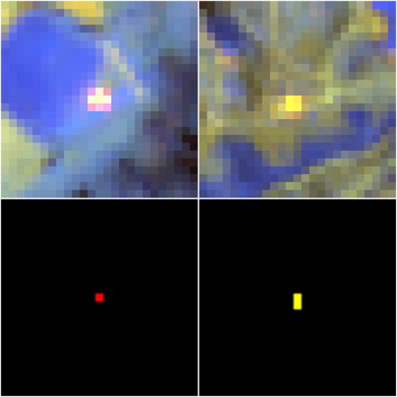
Table 2. Active fire detection algorithm results for the 11 Landsat-8 images (Table 1), where n = number of detected active fire pixels, c = number of detected active fire pixels judged to be commission errors, t = number of pixel locations detected as fire by the three algorithms after commission errors removed, and o = number of active fire detection pixels (selected from t) judged to be omission errors.

Image location	GOLI			Schroeder et al. 2016			Murphy et al. 2016			t
	n	c	o	n	c	o	n	c	o
Australia (Northern Territory)	4950	0	133	3460	0	1623	3423	0	1660	5083
Brazil (State of Rio de Janeiro)	36	4	20	28	5	29	20	0	32	52
Canada (Northwest Territories)	12566	0	2655	8503	0	6718	12573	0	2648	15,221
China (Fujian Province)	25	9	0	34	25	7	16	3	3	16
Germany (Mecklenburg-Vorpommern)	1	0	5	2	0	4	1	0	5	6
Indonesia (Kalimantan)	1951	13	148	1173	11	924	1658	13	441	2086
Indonesia (Sumatra)	84	1	28	53	5	63	64	5	52	111
Iraq (Basrah)	0	0	0	0	0	0	0	0	0	0
Southern Africa (Zimbabwe and Mozambique border)	1617	0	216	1231	0	602	1044	0	789	1833
United States (CA)	3949	3	100	2446	1	1601	3385	2	663	4046
United States (ND)	7	7	0	59	59	0	1	1	0	0

4.2. Modeled probability of active fire detection

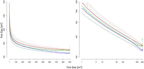
The modeled probability of active fire detection for the GOLI, Schroeder et al. (2016) and Murphy et al. (2016) algorithms plotted as a function of simulated active fire size and temperature are illustrated in Figure 6 to provide insights into their detection omission errors. The results were generated as described below.

Figure 6. Modeled probability of active fire detection for the GOLI (blue), Murphy et al. (2016) (green), and Schroeder et al. (2016) (red) algorithms plotted as a function of simulated active fire size and temperature. The 50% probability is shown as solid and the 10% and 90% probabilities are shown as dotted lines. Simulation results for the four subset images (Figure 1) together are shown with linear (left) and logarithmic (right) scales. Figures appear in color in the online version.

The four Landsat-8 algorithm subset images (Figure 1) were examined and a total of 350 thirty-meter pixels from each image that were visually assessed as not burning were selected. For each selected image pixel, the TOA spectral radiance modeling different active fires sensed through typical atmospheres was simulated (Giglio et al. 2003; Schroeder et al. 2016) as(19) (20) where is the simulated TOA radiance in Landsat-8 band λ (W sr⁻¹ m⁻² m⁻¹) for the pixel that contains fraction (1−f) that is not burning and fraction (f) that is actively burning. The non-burning fraction has a radiance defined by the Landsat-8 radiance of the selected pixel. The burning fraction has a radiance defined by integrating, in 1-nm wavelength steps, the product of the spectral black body emitted radiance (defined as Equation (2)) and the Landsat-8 relative spectral response (RSR_λ) (Barsi et al. 2014; WWW3). Different fire sizes from 1 to 900 m² were modeled in steps of 1 m² (providing different 30-m pixel fire fractions from 0 to 1), and for each the fire temperature was varied from 400 (cool smoldering fire) to 1200 K (hot flaming fire) in steps of 10 K. Atmospheric absorption of the emitted fire radiance was modeled by a spectral atmospheric transmission coefficient ( derived using MODTRAN (Berk et al. 2005) run, assuming a contemporary atmospheric CO₂ concentration of 395 ppm and with image appropriate MODTRAN atmospheric profiles (mid-latitude summer profile for the Canadian image, tropical-urban profile for the Indonesian image, tropical-rural atmospheric profile for the Southern Africa image, US-1976 profile for the US image).

The simulated TOA reflectance was then derived from using the gain and bias conversion coefficients in the Landsat-8 metadata for the corresponding L1T subset image that the pixel was selected from. The simulated TOA reflectance was overwritten into the Landsat-8 subset image at the location that the pixel came from. The GOLI, Murphy et al. (2016) and Schroeder et al. (2016) detection algorithms were then applied to the resulting subset images. For each subset image, and each simulated fire size and temperature combination, the 350 pixel active fire detection results were used to derive the algorithm detection probability as the number of fires (potential or unambiguous) detected in the image divided by 350.

The results considering the four subset images together are shown in Figure 6, reflecting more than 100 million simulations (4 images × 350 pixels per image × 900 fire sizes × 90 fire temperatures), with linear (left) and logarithmic (right) scales. Similar results were found considering the four subset images individually. The 50% probability of active fire detection for each algorithm are shown as solid lines and the 10% and 90% probabilities are shown as dotted lines. Algorithms with lower omission errors will have probabilities that occur closer to the Figure 6 axes. The 50% probabilities for GOLI are closer to the axes than the other algorithms. The GOLI is generally more sensitive than the other two algorithms and the Murphy et al. (2016) algorithm is more sensitive than the Schroeder et al. (2016) algorithm. The fire temperatures and sizes of the German and Brazilian fires (Figure 5) have a 100% probability of active fire detection for all three algorithms. The 50% probability of detection for the smallest simulated fire size of 1 m² occurs when the fire temperature is 1060, 1120, and 1180 K for the GOLI, Murphy et al. (2016), and Schroeder et al. (2016) algorithms, respectively. Typical smoldering 400–500 K fires have less than a 50% detection probability with any algorithm.

The modeled probability of active fire detection provides insights into the omission errors. To check this further, the unambiguous active fires identified in the Canada (Northwest Territories), Southern Africa, US (CA), and Indonesia (Kalimantan) subset images (Section 2.3) were compared to the actual active fire detection results for the three algorithms. The results are shown in Figure 7 on scatterplots of the Landsat-8 bands 5 (0.87 μm), 6 (1.61 μm) and 7 (2.20 μm) reflectance. The top row of Figure 7 shows the TOA reflectance values of the 355 Canadian (green), 77 Indonesian (light blue), 108 Southern African (red), and 256 Californian (dark blue) visually identified unambiguous active fires (total 796). The other rows show the active detection omission errors for the three algorithms. All of the algorithms have omission errors with a total of 104, 157, and 75 of the 796 active fires not detected by the Murphy et al. (2016), Schroeder et al. (2016), and GOLI algorithms, respectively.

Figure 7. Omission error illustration for the Murphy et al. (2016), Schroeder et al. (2016), and GOLI algorithms applied to the unambiguous active fires identified in the Canada (Northwest Territories), Southern Africa, US (CA), and Indonesia (Kalimantan) subset images (Section 2.3). Top row: TOA reflectance values of the 355 Canadian (green), 77 Indonesian (light blue), 108 Southern African (red), and 256 Californian (dark blue) visually identified unambiguous active fire pixel examples. Other rows: the corresponding pixel for each algorithm that were not detected, i.e. the algorithm omission errors. The background gray values show the 39 million CONUS spectral reflectance values (Figure 3) to provide spectral context. Figures appear in color in the online version.

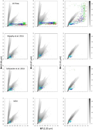
The Murphy et al. (2016) algorithm is elegant but, as seen in Figure 7, is prone to omission errors and fails to detect several active fires with low band 7 (2.20 μm) reflectance. The Schroeder et al. (2016) algorithm is more conservative than the Murphy et al. (2016) algorithm, with a higher omission rate. Detailed inspection indicates that the reflectance thresholds that the Schroeder et al. (2016) criteria use may be too aggressive. This is particularly apparent for some of the Canadian active fires (green) that have low band 7 (2.20 μm) and high band 6 (1.61 μm) active fire reflectance values that are rejected by Equation (10) in the Schroeder et al. (2016) algorithm. In addition, in Equation (6) the threshold on the Landsat-8 shortest wavelength band 1 (blue: 0.44 μm) used by Schroeder et al. (2016) is expected to be very sensitive to atmospheric effects particularly aerosol scattering (Roy et al. 2014b; Vermote et al. 2016). For all three algorithms, the highest omission errors are for the Indonesian peat fires. This is expected from the probability analysis (Figure 6) as smoldering peat fires typically have cool fire temperatures ∼500 K (Elvidge et al. 2015). The GOLI algorithm has fewer omission errors than the other two algorithms. Specifically, the GOLI algorithm omitted to detect 13 of the 355 Canadian fires, 49 of the 77 of the Indonesian fires, 1 of the 108 of the Southern Africa fires, and 12 of the 255 US fires. The reasons for the GOLI omission error differences between images are complex but are driven mainly by the fire size and temperature and the degree of spectral reflectance contrast with the local surroundings.

4.3. Commission and omission errors

The three active fire detection algorithms were applied to the 11 Landsat-8 images (Table 1). Unlike the Schroeder et al. (2016) and GOLI algorithms, the Murphy et al. (2016) algorithm does not include multi-temporal commission error reduction tests. Consequently, the Murphy et al. (2016) results were filtered using the GOLI multi-temporal tests (Equations (17) and (18)) applied to the previous six months of Landsat images.

The active fire detection commission and omission errors are summarized in Table 2 and illustrated in Figures 8 and 9, respectively. The commission errors were first identified by visual interpretation of the detected active fire locations and the Landsat-8 images to locate obvious commission errors (such as fires occurring incorrectly over water bodies). Then, the detections were compared with higher spatial resolution Google Earth imagery acquired before and after the active fire detection date (the date of the Landsat image acquisition). A detection was considered a commission error if it was detected within 30 m of an urban structure or some other feature identified in the Google Earth imagery that could not burn. The n and c values in Table 2 report the number of active fire detections and the number that were commission errors, respectively. The true number of fires that were actively burning in each Landsat image is unknown. For example, very small or cool fires may not be obvious in the Landsat image and the higher spatial resolution Google Earth imagery is rarely acquired at the time of Landsat overpass. Consequently, the spatial union of the active fire detection pixel locations after the commission errors were removed (t in Table 2) was considered to represent the true active fire detection locations. The omission errors for each algorithm were then straightforward to identify by comparison with the spatial union.

Figure 8. Top: Number of pixel locations detected as fire by the three algorithms after commission errors removed (t), bottom: Omission error percentages derived as o/t × 100. Results from Table 2 and the three algorithms shown colored as blue (GOLI), red (Schroeder), and green (Murphy). Figures appear in color in the online version.

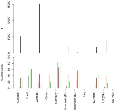
Figure 9. Top: Number of active fire detections (n), bottom: Commission error percentages derived as c/n × 100. Results from Table 2 and the three algorithms are colored blue (GOLI), red (Schroeder), and green (Murphy). Figures appear in color in the online version.

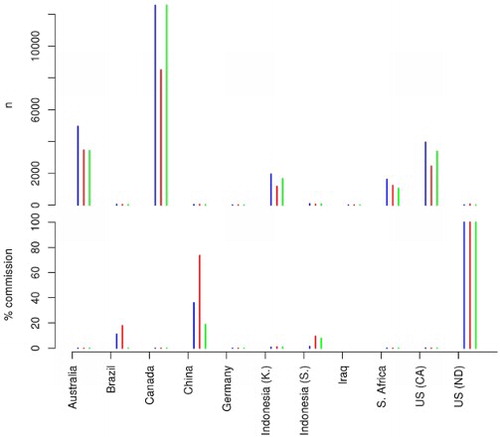
Figure 8 shows the total number of pixel locations detected as fire by the three algorithms after the commission errors were removed (t) and the omission errors expressed as a percentage of t for each algorithm (colors). Smaller colored bars indicate lower omission errors. Among the 11 sites, the GOLI had lower omission errors than the other two algorithms except for Canada and Germany. Over Canada, the GOLI and Murphy algorithms detected a similar number of fires, 12,566 and 12,573, respectively, and the Murphy algorithm had seven less omissions compared than GOLI, which is a marginal difference. The Germany image contained only a single fire event (Figure 5, left) and the GOLI, Schroeder, and Murphy algorithms detected 1, 2, and 1 active fires, respectively, and so the omission statistics for this image are not particularly meaningful. For the same reasons, the omission errors for China, Iraq, and the United States (ND) are less meaningful given their small t values (16, 0, and 0, respectively).

Figure 9 shows the total number of active fire detections detected by each algorithm (n) and the commission errors expressed as a percentage of this number. The top three highest number of active fire detections was in the Canada, Australia, and Southern Africa images, and no commission errors were observed by any of the algorithms. For the other sites, the GOLI had comparable commission errors than the other two algorithms and for most sites the commission error differences were marginal.

The Iraq and US (ND) images were selected as they only encompass gas flares that are expected to cause commission errors. Over the Iraq and US (ND) images, the GOLI algorithm detected 1990 and 604 active fires before and after application of the multi-temporal test, respectively. The multi-temporal test removed all the gas flares over the Iraq and all but 7 over the US (ND) images. The Schroeder and Murphy algorithms had no commission errors after application of the multi-temporal test over the Iraq image and commission errors of 59 and 1, respectively over the US (ND) image. The US (ND) commission errors are likely associated with oil infrastructure building that occurred in the six months prior to the Landsat image acquisition date that are apparent in Google Earth imagery.

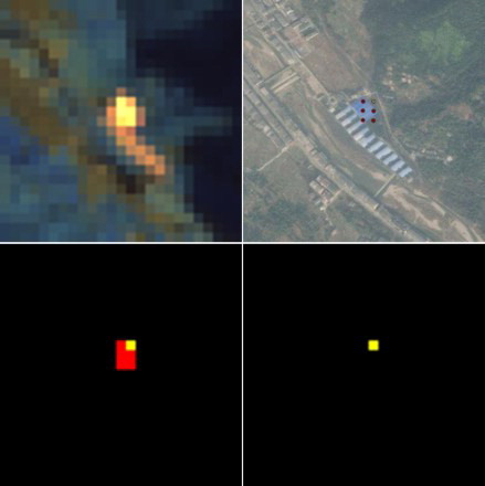
The China image was selected as Schroeder et al. (2016) highlighted it as a particularly problematic source of commission errors due to a large number of buildings with highly reflective building rooftops. Before the multi-temporal test, the GOLI algorithm detected 959 active fires of which the greater majority were clearly commission errors. The GOLI multi-temporal test reduced the number of active fire detections to 25, of which 9 were commission errors. The Schroeder and Murphy algorithms detected 34 and 16 fires after application of the multi-temporal tests and had commission errors of 25 and 3, respectively (Table 2). Figure 10 shows a 25 × 25 thirty-meter pixel subset of the China image with Google Earth imagery and illustrates the GOLI detections before and after the application of the multi-temporal test. It is unlikely that the illustrated GOLI active fire detections are due to vegetation fire. The elevated 2.20, 1.61, 0.87 μm Landsat-8 reflectance corresponds to a row of buildings apparent in the Google Earth image. Perhaps the active fire detections are associated with thermal anomalies caused by building heat exhausts. Similarly, the commission errors over Brazil, Indonesia (Kalimantan and Sumatra), and the United States (CA) were associated primarily with building rooftops. The majority of these commission errors were removed after the application of the multi-temporal tests.

Figure 10. Illustrative 25 × 25 thirty-meter pixel subset (centered on 27.6511°N, 120.1995°E) of the China image (Table 2). Top left: top of atmosphere (TOA) Landsat-8 reflectance (2.20, 1.61, and 0.87 μm shown as red, green, and blue, respectively). Bottom left: GOLI active fire detections without multi-temporal commission reduction. Top right: High-resolution Google Earth imagery sensed after the detection date on 17 January 2015 with active fire detection locations shown as dots. Bottom right: Remaining GOLI active fire detection commission error after the application of the GOLI multi-temporal commission reduction. Figures appear in color in the online version.

5. Conclusions and discussion

This study presented and demonstrated a daytime reflective wavelength Landsat-8 active fire detection algorithm suitable for global application. The GOLI algorithm takes advantage of the improved Landsat-8 calibration, signal-to-noise characteristics, higher 12-bit radiometric resolution, and more precise geolocation compared to previous Landsat sensors (Irons, Dwyer, and Barsi 2012; Roy et al. 2014a). The algorithm builds on heritage active fire detection algorithms with strict (high threshold) per-pixel tests to identify unambiguous active fire pixels and less strict (low threshold) tests to identify potential active fire pixels that are rejected if they do not pass a contextual test. The initial simulations described in this paper illustrate that hotter and larger fires have evident emitted radiation in the longer wavelength Landsat-8 SWIR bands 7 (2.20 μm) and 6 (1.61 μm), less in band 5 (NIR: 0.87 μm), and negligible contribution in band 4 (red: 0.66 μm). Recently, published Landsat-8 algorithms have exploited the greater increase in fire reflectance in Landsat-8 band 7 (2.20 μm) relative to band 5 (0.86 μm) (Murphy et al. 2016; Schroeder et al. 2016). In contrast to the recently published algorithms, the GOLI algorithm uses the significantly greater increase in fire reflectance in band 7 (2.20 μm) relative to band 4 (0.66 μm) to detect unambiguous fires. For all detection algorithms, the definition of the magnitude of change associated with the presence or absence of an actively burning fire is critical. The GOLI algorithm thresholds are fixed and defined statistically by prediction intervals derived considering 39 million reflectance values extracted from 4272 Landsat-8 OLI images acquired over three summer and three winter months across the conterminous United States that capture a range of land cover, land use, vegetation phenology, and soil moisture variations (Roy et al. 2016). The lower 2σ and 3σ prediction intervals for scatterplots of band 4 (0.66 μm) – band 7 (2.20 μm), band 4 (0.66 μm) – band 6 (1.61 μm), and band 6 (1.61 μm) – band 7 (2.20 μm) form the basis for the GOLI detection algorithm. Landsat reflectance saturation has been observed to be considerably less prevalent in Landsat-8 reflectance data compared to previous Landsat sensors due to the improved Landsat-8 sensor design (Roy et al. 2016). However, active fires can emit sufficient radiance to saturate Landsat-8 pixels that complicate active fire detection algorithms, and as with the recently published algorithms, tests for saturation are necessary and implemented.

The development of active fire detection algorithms with low omission errors is trivial if commission errors are ignored. For the majority of active fire applications both low omission and commission errors are required. Even in the fire management community, where the need for rapid fire assessment may be greater than accuracy considerations (Davies et al. 2009), managers do not wish to spend resources visiting satellite detected fires that do not exist (Trigg and Roy 2007). Non-burning surfaces, such as deserts, buildings, clouds, and sun-glint over water, have high reflectance and cause commission errors. The GOLI algorithm uses a similar contextual test as described by Schroeder et al. (2016) but with a growing window dimension rather than a fixed one to compute mean and standard deviation reflectance around each potential active fire detection, similar to the MODIS active fire detection algorithm (Giglio et al. 2003). To further reduce commission errors over highly reflective non-burning surfaces, an additional multi-temporal test is applied. As with Schroeder et al. (2016), the previous six months of Landsat data and past detections are considered, but rather than use a mean six-month band 7 (2.20 μm) reflectance threshold, the GOLI uses the more robust median band 7 (2.20 μm) reflectance in conjunction with thresholds on NDVI to discriminate burning vegetation from non-burning urban surfaces.

Assessment of active fire detection errors is challenging due to difficulties in obtaining independent reference data at the time of satellite overpass. The radiance emitted from an actively burning fire is dependent on the fire temperature and size relative to the non-burning components within the satellite observation (Kaufman et al. 1998; Giglio and Justice 2003) and so for meaningful active fire detection assessment these properties should be known and assessed over a range of conditions. In this study, accuracies were quantified by examination of a sample of Landsat-8 images that encompass a range of burning conditions, including sites that had high and low active fire detection commission errors reported in a recent Landsat-8 active fire detection algorithm study (Schroeder et al. 2016). Clearly, due to the limited number of images used, the accuracy assessments may not portray global accuracies.

Omission errors were quantified using modeled and observed Landsat-8 OLI data over a variety of burning and non-burning surfaces. Comparison of the modeled probability of active fire detection, using realistic simulated scenarios, indicates that the GOLI algorithm has lower omission errors and is able to better detect smaller and cooler fires compared to recently published Landsat-8 algorithms (Schroeder et al. 2016; Murphy et al. 2016). The 50% probability of detection for the smallest simulated fire size of 1 m² occurred when the fire temperature was 1060, 1120, and 1180 K for the GOLI, Murphy et al. (2016), and Schroeder et al. (2016) algorithms, respectively. This pattern of lower omission errors was corroborated by inspection of the algorithm results applied to 11 Landsat-8 test images.

Assessment of active fire detection commission errors is particularly hard to undertake as false active fire detection is difficult to identify reliably. Eleven Landsat-8 test images and corresponding Google Earth  high-resolution imagery acquired before and after the image acquisition dates were examined visually to exhaustively check for commission errors. The greatest number of active fire detections was in the Canada, Australia, and Southern Africa images, and no commission errors were observed by any of the algorithms, indicating that the GOLI multi-temporal commission reduction tests were not overly aggressive. Despite this, commission errors remained in several of the other test images, and were predominantly associated with buildings. This source of commission error is not documented in the MODIS 1-km active fire detection product but is evident in 375-m visible infrared imaging radiometer suite active fire products (Schroeder et al. 2014). As noted by Schroeder et al. (2016), this is a difficult issue to resolve. In particular, buildings that were built in the six months prior to the fire detection and/or specular reflectance off building roof tops that only occurred on the fire detection image and not in the previous six months of images may be difficult to unambiguously identify and remove. A contemporaneous high spatial resolution land cover map may help resolve this issue; however, in urban areas, land cover classification with Landsat data is often unreliable (Li, Gong, and Liang 2015; Zhang and Roy 2017), and there were no 30 m or higher spatial resolution year 2014 land cover maps available for this study.

The Landsat sensors were not designed for active fire monitoring. Landsat active fire detection algorithms are sub-optimal as they must use reflective wavelength data and not middle-infrared and thermal infrared wavelengths that are better suited to detecting fires (Dozier 1981; Kaufman et al. 1998; Giglio et al. 2003; Wooster, Xu, and Nightingale 2012). Despite this, the expectation of continued Landsat missions – notably Landsat-9 will be a clone of Landsat-8, and Landsat-10 will have improved capabilities while preserving measurement continuity (Loveland and Irons 2016) – underpins the need for research in this domain. Until there are several Landsat sensors in orbit concurrently, the utility of Landsat active fire detection, beyond providing moderate spatial resolution snap-shots of fire activity every 16-day repeat, is limited by the temporal sampling (Roy et al. 2014a). However, the Sentinel 2 sensors (Drusch et al. 2012), with one sensor in orbit since 2015 and another launched in 2017, have Landsat-like reflectance bands suitable for burned area mapping (Huang et al. 2016) and include similar reflective wavelength bands to those used by the GOLI, Schroeder et al. (2016), and Murphy et al. (2016) algorithms. Fusion of Landsat-8 and Sentinel-2 satellites therefore provides the potential for moderate resolution active fire monitoring with near daily temporal resolution (Li and Roy 2017), augmenting daily global active fire monitoring and characterization provided by coarser spatial resolution polar and geostationary systems.

Disclosure statement

No potential conflict of interest was reported by the authors.

ORCID

S. S. Kumar http://orcid.org/0000-0003-4067-4926

D. P. Roy http://orcid.org/0000-0002-1347-0250

Additional information

Funding

This research was funded by the NASA Land Cover/Land Use Change (LCLUC14-2): Multi-Source Land Imaging Science Program, Grant [NNX15AK94G] and by the U.S. Department of Interior, U.S. Geological Survey (USGS) under grant [G12PC00069].

References

- Aragão, L. E. O. C., Y. Malhi, R. M. Roman-Cuesta, S. Saatchi, L. O. Anderson, and Y. E. Shimabukuro. 2007. “Spatial Patterns and Fire Response of Recent Amazonian Droughts.” Geophysical Research Letters 34. doi: 10.1029/2006GL028946
- Barsi, J. A., K. Lee, G. Kvaran, B. L. Markham, and J. A. Pedelty. 2014. “The Spectral Response of the Landsat-8 Operational Land Imager.” Remote Sensing 6: 10232–10251. doi:10.3390/rs61010232.
- Berk, A., G. P. Anderson, P. K. Acharya, L. S. Bernstein, L. Muratov, J. Lee, M. Fox, S. M. Adler-Golden, J. H. Chetwynd, and M. L. Hoke. 2005. “MODTRAN 5: A Reformulated Atmospheric Band Model with Auxiliary species and Practical Multiple Scattering Options: Update.” In Defense and Security, 662–667. Orlando, FL: International Society for Optics and Photonics.
- Boschetti, L., and D. P. Roy. 2008. “Defining a Fire Year for Reporting and Analysis of Global Interannual Fire Variability.” Journal of Geophysical Research: Biogeosciences (2005–2012) 113. doi: 10.1029/2008JG000686
- Boschetti, L., D. P. Roy, C. O. Justice, and M. Humber. 2015. “MODIS-Landsat Fusion for Large Area 30m Burned Area Mapping.” Remote Sensing of Environment 161: 27–42. doi:10.1016/j.rse.2015.01.022.
- Boschetti, L., S. V. Stehman, and D. P. Roy. 2016. “A Stratified Random Sampling Design in Space and Time for Regional to Global Scale Burned Area Product Validation.” Remote Sensing of Environment 186: 465–478. doi:10.1016/j.rse.2016.09.016.
- Bowman, D. M., J. K. Balch, P. Artaxo, W. J. Bond, J. M. Carlson, M. A. Cochrane, C. M. D’Antonio, R. S. DeFries, J. C. Doyle, and S. P. Harrison. 2009. “Fire in the Earth System.” Science 324: 481–484. doi:10.1126/science.1163886.
- Cardoso, M. F., G. C. Hurtt, B. Moore, C. A. Nobre, and H. Bain. 2005. “Field Work and Statistical Analyses for Enhanced Interpretation of Satellite Fire Data.” Remote Sensing of Environment 96: 212–227. doi:10.1016/j.rse.2005.02.008.
- Chuvieco, E., L. Giglio, and C. Justice. 2008. “Global Characterization of Fire Activity: Toward Defining Fire Regimes from Earth Observation Data.” Global Change Biology 14: 1488–1502. doi:10.1111/j.1365-2486.2008.01585.x.
- Cocke, A. E., P. Z. Fulé, and J. E. Crouse. 2005. “Comparison of Burn Severity Assessments Using Differenced Normalized Burn Ratio and Ground Data.” International Journal of Wildland Fire 14: 189–198. doi:10.1071/WF04010.
- Csiszar, I. A., J. T. Morisette, and L. Giglio. 2006. “Validation of Active Fire Detection from Moderate-resolution Satellite Sensors: The MODIS Example in Northern Eurasia.” IEEE Transactions on Geoscience and Remote Sensing 44: 1757–1764. doi:10.1109/TGRS.2006.875941.
- Csiszar, I. A., and W. Schroeder. 2008. “Short-term Observations of the Temporal Development of Active Fires from Consecutive Same-day ETM+ and ASTER Imagery in the Amazon: Implications for Active Fire Product Validation.” IEEE Journal of Selected Topics in Applied Earth Observations and Remote Sensing 1: 248–253. doi:10.1109/JSTARS.2008.2011377.
- Davies, A. G., S. Chien, V. Baker, T. Doggett, J. Dohm, R. Greeley, F. Ip, et al. 2006. “Monitoring Active Volcanism with the Autonomous Sciencecraft Experiment on EO-1.” Remote Sensing of Environment 101: 427–446. doi:10.1016/j.rse.2005.08.007.
- Davies, D. K., S. Ilavajhala, M. M. Wong, and C. O. Justice. 2009. “Fire Information for Resource Management System: Archiving and Distributing MODIS Active Fire Data.” IEEE Transactions on Geoscience and Remote Sensing 47: 72–79. doi:10.1109/TGRS.2008.2002076.
- De Moura, M. L., and L. S. Galvão. 2003. “Smoke Effects on NDVI Determination of Savannah Vegetation Types.” International Journal of Remote Sensing 24: 4225–4231. doi:10.1080/0143116031000152318.
- Dozier, J. 1981. “A Method for Satellite Identification of Surface Temperature Fields of Subpixel Resolution.” Remote Sensing of Environment 11: 221–229. doi:10.1016/0034-4257(81)90021-3.
- Drusch, M., U. Del Bello, S. Carlier, O. Colin, V. Fernandez, F. Gascon, B. Hoersch, C. Isola, P. Laberinti, and P. Martimort. 2012. “Sentinel-2: ESA’s Optical High-resolution Mission for GMES Operational Services.” Remote Sensing of Environment 120: 25–36. doi:10.1016/j.rse.2011.11.026.
- Elvidge, C. D., M. Zhizhin, F.-C. Hsu, K. Baugh, M. R. Khomarudin, Y. Vetrita, P. Sofan, and D. Hilman. 2015. “Long-wave Infrared Identification of Smoldering Peat Fires in Indonesia with Nighttime Landsat Data.” Environmental Research Letters 10: 065002. doi: 10.1088/1748-9326/10/6/065002
- FEMA 2005. “ The Seasonal Nature of Fires.” In Emmitsburg, MD.: Federal Emergency Management Agency (FEMA). Accessed May 2017. https://www.usfa.fema.gov/downloads/pdf/publications/fa-236.pdf.
- Flasse, S., and P. Ceccato. 1996. “A Contextual Algorithm for AVHRR Fire Detection.” International Journal of Remote Sensing 17: 419–424. doi:10.1080/01431169608949018.
- Fraser, R., Z. Li, and J. Cihlar. 2000. “Hotspot and NDVI Differencing Synergy (HANDS) A New Technique for Burned Area Mapping Over Boreal Forest.” Remote Sensing of Environment 74: 362–376. 10.1016/S0034-4257(00)00078-X.
- French, N. H. F., E. S. Kasischke, R. J. Hall, K. A. Murphy, D. L. Verbyla, E. E. Hoy, and J. L. Allen. 2008. “Using Landsat Data to Assess Fire and Burn Severity in the North American Boreal Forest Region: An Overview and Summary of Results.” International Journal of Wildland Fire 17: 443–462. doi:10.1071/WF08007.
- Frost, P. 2013. “ Mobile Application Launched for the Advanced Fire Information System.” Accessed May 2017. Retrieved 2014 from CSIR: http://www.csir.co.za/enews/2013_oct/25.html.
- Giglio, L. 2007. “Characterization of the Tropical Diurnal Fire Cycle Using VIRS and MODIS Observations.” Remote Sensing of Environment 108: 407–421. doi:10.1016/j.rse.2006.11.018.
- Giglio, L., I. Csiszar, Á Restás, J. T. Morisette, W. Schroeder, D. Morton, and C. O. Justice. 2008. “Active Fire Detection and Characterization with the Advanced Spaceborne Thermal Emission and Reflection Radiometer (ASTER).” Remote Sensing of Environment 112: 3055–3063. doi:10.1016/j.rse.2008.03.003.
- Giglio, L., J. Descloitres, C. O. Justice, and Y. J. Kaufman. 2003. “An Enhanced Contextual Fire Detection Algorithm for MODIS.” Remote Sensing of Environment 87: 273–282. doi:10.1016/S0034-4257(03)00184-6.
- Giglio, L., and C. Justice. 2003. “Effect of Wavelength Selection on Characterization of Fire Size and Temperature.” International Journal of Remote Sensing 24: 3515–3520. doi:10.1080/0143116031000117056.
- Giglio, L., T. Loboda, D. P. Roy, B. Quayle, and C. O. Justice. 2009. “An Active-fire Based Burned Area Mapping Algorithm for the MODIS Sensor.” Remote Sensing of Environment 113: 408–420. doi:10.1016/j.rse.2008.10.006.
- Goward, S., T. Arvidson, D. Williams, J. Faundeen, J. Irons, and S. Franks. 2006. “Historical Record of Landsat Global Coverage: Mission Operations, NSLRSDA, and International Cooperator Stations.” Photogrammetric Engineering and Remote Sensing 72: 1155. doi: 10.14358/PERS.72.10.1155
- Huang, H., D. P. Roy, B. Boschetti, H. K. Zhang, L. Yan, S. S. Kumar, J. Gomez-Dans, and J. Li. 2016. “Separability Analysis of Sentinel-2A Multi-spectral Instrument (MSI) Data for Burned Area Discrimination.” Remote Sensing 8 (10): 873. doi: 10.3390/rs8100873
- Irons, J. R., J. L. Dwyer, and J. A. Barsi. 2012. “The Next Landsat Satellite: The Landsat Data Continuity Mission.” Remote Sensing of Environment 122: 11–21. doi:10.1016/j.rse.2011.08.026.
- Ju, J., and D. P. Roy. 2008. “The Availability of Cloud-free Landsat ETM+ Data Over the Conterminous United States and Globally.” Remote Sensing of Environment 112: 1196–1211. doi:10.1016/j.rse.2007.08.011.
- Ju, J., D. P. Roy, E. Vermote, J. Masek, and V. Kovalskyy. 2012. “Continental-scale Validation of MODIS-Based and LEDAPS Landsat ETM+ Atmospheric Correction Methods.” Remote Sensing of Environment 122: 175–184. doi:10.1016/j.rse.2011.12.025.
- Kaiser, J., A. Heil, M. Andreae, A. Benedetti, N. Chubarova, L. Jones, J.-J. Morcrette, M. Razinger, M. Schultz, and M. Suttie. 2012. “Biomass Burning Emissions Estimated with a Global Fire Assimilation System Based on Observed Fire Radiative Power.” Biogeosciences (online) 9: 527–554. doi:10.5194/bg-9-527-2012.
- Kaufman, Y. J., C. O. Justice, L. P. Flynn, J. D. Kendall, E. M. Prins, L. Giglio, D. E. Ward, W. P. Menzel, and A. W. Setzer. 1998. “Potential Global Fire Monitoring from EOS-MODIS.” Journal of Geophysical Research 103.
- Kovalskyy, V., and D. P. Roy. 2015. “A one Year Landsat 8 Conterminous United States Study of Cirrus and Non-cirrus Clouds.” Remote Sensing 7: 564–578. doi:10.3390/rs70100564.
- Kumar, S., D. Roy, L. Boschetti, and R. Kremens. 2011. “Exploiting the Power law Distribution Properties of Satellite Fire Radiative Power Retrievals: A Method to Estimate Fire Radiative Energy and Biomass Burned from Sparse Satellite Observations.” Journal of Geophysical Research: Atmospheres 116.
- Kumar, S. S., D. P. Roy, M. A. Cochrane, C. M. Souza JR, C. Barber, and L. Boschetti. 2014. “A Quantitative Study of the Proximity of Satellite Detected Active Fires to Roads and Rivers in the Brazilian Tropical Moist Forest Biome.” International Journal of Wildland Fire 23 (4): 532–543. doi:10.1071/WF13106.
- Lentile, L. B., Z. A. Holden, A. M. Smith, M. J. Falkowski, A. T. Hudak, P. Morgan, S. A. Lewis, P. E. Gessler, and N. C. Benson. 2006. “Remote Sensing Techniques to Assess Active Fire Characteristics and Post-fire Effects.” International Journal of Wildland Fire 15: 319–345. doi:10.1071/WF05097.
- Li, X., P. Gong, and L. Liang. 2015. “A 30-year (1984–2013) Record of Annual Urban Dynamics of Beijing City Derived from Landsat Data.” Remote Sensing of Environment 166: 78–90. doi:10.1016/j.rse.2015.06.007.
- Li, J., and D. P. Roy. 2017. “A Global Analysis of Sentinel-2A, Sentinel-2B and Landsat-8 Data Revisit Intervals and Implications for Terrestrial Monitoring.” Remote Sensing 9 (9): 902. doi: 10.3390/rs9090903
- Loboda, T. V., and I. A. Csiszar. 2007. “Reconstruction of Fire Spread within Wildland Fire Events in Northern Eurasia from the MODIS Active Fire Product.” Global and Planetary Change 56: 258–273. doi:10.1016/j.gloplacha.2006.07.015.
- Loveland, T. R., and J. L. Dwyer. 2012. “Landsat: Building a Strong Future.” Remote Sensing of Environment 122: 22–29. doi:10.1016/j.rse.2011.09.022.
- Loveland, T. R., and J. R. Irons. 2016. “Landsat 8: The Plans, the Reality, and the Legacy.” Remote Sensing of Environment 185: 1–6. doi:10.1016/j.rse.2016.07.033.
- Lymburner, L., E. Botha, E. Hestir, J. Anstee, S. Sagar, A. Dekker, and T. Malthus. 2016. “Landsat 8: Providing Continuity and Increased Precision for Measuring Multi-decadal Time Series of Total Suspended Matter.” Remote Sensing of Environment 185: 108–118. doi:10.1016/j.rse.2016.04.011.
- Markham, B., J. Barsi, G. Kvaran, L. Ong, E. Kaita, S. Biggar, J. Czapla-Myers, N. Mishra, and D. Helder. 2014. “Landsat-8 Operational Land Imager Radiometric Calibration and Stability.” Remote Sensing 6: 12275–12308. doi:10.3390/rs61212275.
- Matson, M., and J. Dozier. 1981. “Identification of Subresolution High Temperature Sources Using a Thermal IR Sensor.” Photogrammetric Engineering and Remote Sensing 47 (9): 1311–1318.
- Micijevic, E., K. Vanderwerff, P. Scaramuzza, R. A. Morfitt, J. A. Barsi, and R. Levy. 2014. “On-orbit Performance of the Landsat 8 Operational Land Imager.” In SPIE Optical Engineering+ Applications, 921816–921812. San Diego, CA: International Society for Optics and Photonics.
- Montanaro, M., A. Gerace, A. Lunsford, and D. Reuter. 2014. “Stray Light Artifacts in Imagery from the Landsat 8 Thermal Infrared Sensor.” Remote Sensing 6: 10435–10456. doi: 10.3390/rs61110435
- Morfitt, R., J. Barsi, R. Levy, B. Markham, E. Micijevic, L. Ong, P. Scaramuzza, and K. Vanderwerff. 2015. “Landsat-8 Operational Land Imager (OLI) Radiometric Performance on-Orbit.” Remote Sensing 7: 2208–2237. doi:10.3390/rs70202208.
- Morisette, J. T., L. Giglio, I. Csiszar, and C. O. Justice. 2005a. “Validation of the MODIS Active Fire Product Over Southern Africa with ASTER Data.” International Journal of Remote Sensing 26: 4239–4264. doi:10.1080/01431160500113526.
- Morisette, J. T., L. Giglio, I. Csiszar, A. Setzer, W. Schroeder, D. Morton, and C. O. Justice. 2005b. “Validation of MODIS Active Fire Detection Products Derived from two Algorithms.” Earth Interactions 9: 1–25. doi:10.1175/EI141.1.
- Murphy, S. W., C. R. de Souza Filho, R. Wright, G. Sabatino, and R. C. Pabon. 2016. “HOTMAP: Global hot Target Detection at Moderate Spatial Resolution.” Remote Sensing of Environment 177: 78–88. doi:10.1016/j.rse.2016.02.027.
- Oppenheimer, C. 1991. “Lava Flow Cooling Estimated from Landsat Thematic Mapper Infrared Data: The Lonquimay Eruption (Chile, 1989).” Journal of Geophysical Research: Solid Earth 96: 21865–21878. doi:10.1029/91JB01902.
- Pahlevan, N., Z. Lee, J. Wei, C. B. Schaaf, J. R. Schott, and A. Berk. 2014. “On-orbit Radiometric Characterization of OLI (Landsat-8) for Applications in Aquatic Remote Sensing.” Remote Sensing of Environment 154: 272–284. doi:10.1016/j.rse.2014.08.001.
- Pereira, J. M., D. Oom, P. Pereira, A. A. Turkman, and K. F. Turkman. 2015. “Religious Affiliation Modulates Weekly Cycles of Cropland Burning in Sub-Saharan Africa.” PloS one 10 (9): e0139189. doi: 10.1371/journal.pone.0139189
- Peterson, D., J. Wang, C. Ichoku, E. Hyer, and V. Ambrosia. 2013. “A Sub-pixel-based Calculation of Fire Radiative Power from MODIS Observations: 1: Algorithm Development and Initial Assessment.” Remote Sensing of Environment 129: 262–279. doi: 10.1016/j.rse.2012.10.036
- Prins, E. M., and W. P. Menzel. 1992. “Geostationary Satellite Detection of Biomass Burning in South America.” International Journal of Remote Sensing 13: 2783–2799. doi:10.1080/01431169208904081.
- Pyne, S. J., P. Andrews, and R. Laven. 1996. Introduction to Wildland fire (Second Edition). New York: John Wiley and Sons, Inc.
- Roberts, G. J., and M. J. Wooster. 2008. “Fire Detection and Fire Characterization Over Africa using Meteosat SEVIRI.” IEEE Transactions on Geoscience and Remote Sensing 46: 1200–1218. doi:10.1109/TGRS.2008.915751.
- Robinson, J. M. 1991. “Fire from Space: Global Fire Evaluation Using Infrared Remote Sensing.” International Journal of Remote Sensing 12: 3–24. doi:10.1080/01431169108929628.
- Roy, D. P., L. Giglio, J. D. Kendall, and C. O. Justice. 1999. “Multi-temporal Active-fire Based Burn Scar Detection Algorithm.” International Journal of Remote Sensing 20: 1031–1038. 10.1080/014311699213073.
- Roy, D. P., V. Kovalskyy, H. K. Zhang, E. F. Vermote, L. Yan, S. S. Kumar, and A. Egorov. 2016. “Characterization of Landsat-7 to Landsat-8 Reflective Wavelength and Normalized Difference Vegetation Index Continuity.” Remote Sensing of Environment 185: 57–70. doi:10.1016/j.rse.2015.12.024.
- Roy, D. P., and S. S. Kumar. 2017. “Multi-year MODIS Active Fire Type Classification Over the Brazilian Tropical Moist Forest Biome.” International Journal of Digital Earth 10 (1): 54–84. doi: 10.1080/17538947.2016.1208686
- Roy, D. P., Y. Qin, V. Kovalskyy, E. F. Vermote, J. Ju, A. Egorov, M. C. Hansen, I. Kommareddy, and L. Yan. 2014a. “Conterminous United States Demonstration and Characterization of MODIS-based Landsat ETM+ Atmospheric Correction.” Remote Sensing of Environment 140: 433–449. doi: 10.1016/j.rse.2013.09.012
- Roy, D. P., M. A. Wulder, T. R. Loveland, C. E. Woodcock, R. G. Allen, M. C. Anderson, D. Helder, et al. 2014b. “Landsat-8: Science and Product Vision for Terrestrial Global Change Research.” Remote Sensing of Environment 145: 154–172. doi: 10.1016/j.rse.2014.02.001
- Saxon, E., and Sheppard, S. 2010. “ Land Systems of Indonesia and Papua New Guinea.” Last Accessed May 2017. http://www.arcgis.com/home/item.html?id=dae887c070b840e1bdae639a1e63260d.
- Schaepman-Strub, G., M. Schaepman, T. Painter, S. Dangel, and J. Martonchik. 2006. “Reflectance Quantities in Optical Remote Sensing—Definitions and Case Studies.” Remote Sensing of Environment 103: 27–42. doi:10.1016/j.rse.2006.03.002.
- Schroeder, W., J. T. Morisette, I. Csiszar, L. Giglio, D. Morton, and C. O. Justice. 2005. “Characterizing Vegetation Fire Dynamics in Brazil Through Multisatellite Data: Common Trends and Practical Issues.” Earth Interactions 9: 1–26. doi:10.1175/EI120.1.
- Schroeder, W., P. Oliva, L. Giglio, and I. A. Csiszar. 2014. “The New VIIRS 375 m Active Fire Detection Data Product: Algorithm Description and Initial Assessment.” Remote Sensing of Environment 143: 85–96. doi:10.1016/j.rse.2013.12.008.
- Schroeder, W., P. Oliva, L. Giglio, B. Quayle, E. Lorenz, and F. Morelli. 2016. “Active Fire Detection Using Landsat-8/OLI Data.” Remote Sensing of Environment 185: 210–220. doi:10.1016/j.rse.2015.08.032.
- Schroeder, W., E. Prins, L. Giglio, I. Csiszar, C. Schmidt, J. Morisette, and D. Morton. 2008. “Validation of GOES and MODIS Active Fire Detection Products Using ASTER and ETM+ Data.” Remote Sensing of Environment 112: 2711–2726. doi:10.1016/j.rse.2008.01.005.
- Siegert, F., B. Zhukov, D. Oertel, S. Limin, S. E. Page, and J. O. Rieley. 2004. “Peat Fires Detected by the BIRD Satellite.” International Journal of Remote Sensing 25: 3221–3230. doi:10.1080/01431160310001642377.
- Storey, J., M. Choate, and K. Lee. 2014. “Landsat 8 Operational Land Imager On-orbit Geometric Calibration and Performance.” Remote Sensing 6: 11127–11152. doi:10.3390/rs61111127.
- Stroppiana, D., S. Pinnock, and J. M. Gregoire. 2000. “The Global Fire Product: Daily Fire Occurrence from April 1992 to December 1993 Derived from NOAA AVHRR Data.” International Journal of Remote Sensing 21 (6-7): 1279–1288. doi:10.1080/014311600210173.
- Swap, R. J., H. J. Annegarn, J. T. Suttles, J. Haywood, M. C. Helmlinger, C. Hely, P. V. Hobbs, et al. 2002. “The Southern African Regional Science Initiative (SAFARI 2000): Overview of the Dry-season Field Campaign.” South African Journal of Science 98: 125–130.
- Trigg, S. N., and D. P. Roy. 2007. “A Focus Group Study of Factors that Promote and Constrain the Use of Satellite Derived Fire Products by Resource Managers in Southern Africa.” Journal of Environmental Management 82: 95–110. doi:10.1016/j.jenvman.2005.12.008.
- Vermote, E. F., C. O. Justice, M. Claverie, and B. Franch. 2016. “Preliminary Analysis of the Performance of the Landsat 8/OLI Land Surface Reflectance Product.” Remote Sensing of Environment 185: 46–56. doi:10.1016/j.rse.2016.04.008.
- Weisberg, S. 2005. Applied Linear Regression. Hoboken, NJ: Wiley.
- Wooster, M. J., W. Xu, and T. Nightingale. 2012. “Sentinel-3 SLSTR Active Fire Detection and FRP Product: Pre-launch Algorithm Development and Performance Evaluation Using MODIS and ASTER Datasets.” Remote Sensing of Environment 120: 236–254. doi:10.1016/j.rse.2011.09.033.
- Wulder, M. A., J. C. White, T. R. Loveland, C. E. Woodcock, A. S. Belward, W. B. Cohen, G. Fosnight, J. Shaw, J. G. Masek, and D. P. Roy. 2016. “The Global Landsat Archive: Status, Consolidation, and Direction.” Remote Sensing of Environment 185: 271–283. doi:10.1016/j.rse.2015.11.032.
- WWW2 ASTM Standard Extraterrestrial Spectrum Reference E-490-00. Accessed May 2017. http://rredc.nrel.gov/solar/spectra/am0/.
- WWW1 (Joint Fire Science Program). Accessed May 2017. https://www.frames.gov/partner-sites/assessing-burn-severity/spectral/
- WWW3 Spectral Response of the Operational Land Imager In-Band, Band-Average Relative Spectral Response. Accessed May 2017. http://landsat.gsfc.nasa.gov/?p=5779.
- Zhang, X., S. Kondragunta, and D. P. Roy. 2014. “Interannual Variation in Biomass Burning and Fire Seasonality Derived from Geostationary Satellite Data Across the Contiguous United States from 1995 to 2011.” Journal of Geophysical Research: Biogeosciences 119: 1147–1162. doi:10.1002/2013JG002518.
- Zhang, H. K., and D. P. Roy. 2017. “Using the 500 m MODIS Land Cover Product to Derive a Consistent Continental Scale 30 m Landsat Land Cover Classification.” Remote Sensing of Environment 197: 15–34. doi:10.1016/j.rse.2017.05.024.
- Zhang, H. K., D. P. Roy, and V. Kovalskyy. 2016. “Optimal Solar Geometry Definition for Global Long Term Landsat Time Series Bi-directional Reflectance Normalization.” IEEE Transactions on Geoscience and Remote Sensing 54 (3): 1410–1418. doi: 10.1109/TGRS.2015.2480684