2014 summer Arctic sea ice thickness and concentration from shipborne observations

ABSTRACT

A series of shipborne sea ice observations were performed during the Chinese National Arctic Research Expedition in the Pacific Arctic sector between 2 August 2014 and 1 September 2014. Undeformed sea ice thickness (SIT) as well as area fractions of open water, melt pond, and sea ice (A_w, A_p, and A_i) were monitored using downward-oriented and oblique-oriented cameras. The results show that SIT varied between 20 and 220 cm throughout the whole cruise, with the average and standard deviation equaling 104.9 and 29.1 cm, respectively. Mean A_w and A_i were 0.52 and 0.44 in the marginal ice zone, respectively, while mean A_w decreased to 0.23 and mean A_i increased to 0.73 in the pack ice zone. Limited variation between 0 and 0.32 in A_p was seen throughout the whole cruise. Shipborne sea ice concentration was then rectified and mapped across a large transect to validate estimates derived from the satellite sensors Special Sensor Microwave Imager/Sounder (SSMIS) (25 km) and AMSR2 (25 km). Overestimations were 9.5% and 9.9% for SSMIS and AMSR2 compared with measurements, respectively. The mean areal broadband surface albedo based on shipborne survey increased from 0.07 to 0.66 along the transect between 72°N and 81°N.

KEYWORDS:

• Arctic sea ice
• shipborne photography
• remote sensing
• surface albedo
• summer melt

1. Introduction

The Arctic plays a vital role in the climate system, as one of the Earth’s ‘three poles’ in addition to the Antarctic and the Qinghai-Tibet Plateau. However, data show that Arctic air temperature has increased at a speed more than twice the global rate because of the Arctic Amplification (Serreze and Barry 2011), while Arctic sea ice in this ocean has experienced dramatic changes in recent decades, including a consistent reduction in extent (Comiso et al. 2008; Stroeve et al. 2012), loss of multi-year coverage (Kwok and Cunningham 2010; Comiso 2012), and a reduction in thickness (Renner et al. 2014; Lindsay and Schweiger 2015). These changes have caused large fluctuations in the sea ice regime, leading to possible navigations as the Arctic ocean has become more accessible (Khon and Mokhov 2010; Liu and Kronbak 2010; Shibata et al. 2013). In each summer of recent years, Chinese container vessels have been able to pass through the Arctic passage to Europe. Indeed, subsequent to the proposal and future development of the Belt and Road Initiative, Arctic navigations between China and Europe is expanding.

Thus, it is now especially important to study Arctic sea ice, especially the vital parameters of sea ice concentration (SIC) and sea ice thickness (SIT). These variables are important, not only as measures for the state of the climate, but also for Arctic navigations. SIC is the main variable affecting the composite surface albedo of the Arctic Ocean, and SIT affects the heat budget of the Arctic and exchanges of freshwater between sea ice and the ocean. Variation in these parameters along a cruise also influences the probability of Arctic sailing, as both are related to the ice load exerted on the hull of a ship and thus are crucial factors in determining whether a vessel can break through the ice zone or not.

Remote sensing (RS) is an important approach that can be applied to measure sea ice conditions at the pan-Arctic scale. Indeed, since the launch of the Electronically Scanning Microwave Radiometer in late 1972, data on Arctic ice conditions have been readily available almost continuously from space-borne instruments. And since 1978, more data have been commonly acquired by the Special Sensor Microwave/Imager (SSM/I) and Special Sensor Microwave Imager/Sounder (SSMIS). Applying the NASA Team (NT) algorithm, these RS data are able to provide a consistent SIC time series at a spatial resolution of 25 km. A further satellite instrument, the Advanced Microwave Scanning Radiometer for the Earth Observing System (AMSR-E), has also been operational since 2002, and its successor (AMSR-2) started acquiring data in 2012. The climate change initiative sea ice (SICCI) project collected SIC measurements from AMSR2 data at resolutions of 25 and 50 km since 2012. However, available passive microwave SIC reveals a significant difference compared with in situ data because of the coarse spatial resolution distinguishing small-scale open water and melt ponds (Inoue, Curry, and Maslanik 2008; Li et al. 2017). In addition, SIC retrieved from passive microwave data using different algorithms is shown to be different compared with each other (Spreen, Kaleschke, and Heygster 2008; Ivanova et al. 2014; Beitsch, Kern, and Kaleschke 2015). In situ observation of sea ice conditions is therefore essential to validate RS SIC.

Several methods are available for field observations of sea ice conditions. Ice cores were drilled and measured to determine the ice thickness of an area in many previous expeditions (Overgaard, Wadhams, and Leppäranta 1983; Perovich et al. 2009; Xie et al. 2013). While this method could not give the ice thickness in a wide region, manual visual observation has been widely conducted to record the sea ice conditions along the vessel route in the Southern Ocean (Worby and Allison 1999; Knuth and Ackley 2006; Worby et al. 2008; Tekeli et al. 2011) and Arctic Ocean (|Lei et al. 2012, 2017; Xie et al. 2013). Shipborne and airborne investigations were then conducted to avoid the possible errors in visual method and collect more consecutive data (Weissling et al. 2009; Lu et al. 2010; Istomina et al. 2015; Miao et al. 2015; Huang et al. 2016; Lu et al. 2016b). Instruments, such as digital cameras, are utilized to capture images of sea ice conditions onboard a ship or aircraft. Algorithms of image processing are then applied post hoc to retrieve ice thickness and morphology on the basis of these images (Lu and Li 2010; Zhang and Skjetne 2015; Lu et al. 2016b). Several other instruments, such as electromagnetic device (Haas et al. 2009) and laser altimeter (Kurtz et al. 2008) were previously adopted on ship and airplane to measure ice thickness and freeboard.

All above field investigation methods enable the recording of small-scale ice features that are undetectable by satellites. Furthermore, with a purpose of continuous and efficient observations, shipborne photography is superior compared with the other field methods because of its cost effectiveness, automatic operation, and high level of accuracy. Using this observation method, ice conditions along ship cruise were recorded in the Arctic Ocean during 2014 summer.

As part of the Chinese National Arctic Research Expedition in 2014 (CHINARE-2014), R/V Xuelong sailed during summer in the ice zone of the Pacific Arctic sector and carried out shipborne observations for SIT and SIC. The aim of this paper is to present and illustrate the SIT measurements as well as the sea ice morphology and SIC data collected during this cruise. These data are all potentially useful for future Arctic navigations and might guide the development of a future systematic data base, as we intend to propose a reliable shipborne method to measure ice conditions during a cruise which could be applied to all ships sailing in the Arctic. The measurements presented in this paper can thus be regarded as basic data for validating information from satellites. Another aim is to develop an approach to pinpoint SIC over large scales utilizing local scale data.

2. Observations and data

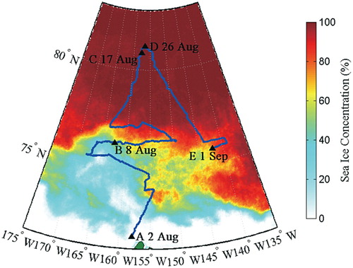
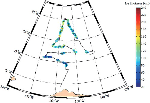
The trajectory of observation within the ice zone during the CHINARE-2014 cruise is shown in Figure 1. Observation of the ice conditions was initiated at around 72°N (A) in the offshore region near Barrow on 2 August 2014. The vessel sailed within the marginal ice zone (MIZ) before it reached the pack ice zone (PIZ) at around 76°N (B) on 8 August 2014. Once inside the PIZ the vessel reached 80.8°N (C) on 17 August 2014 and settled there for long-term ice camp (LIC) of nine days. The vessel subsequently drifted northward to 81.2°N (D) by the end of the LIC, and began the backward trip on 26 August 2014. Thus, by 1 September 2014, the R/V Xuelong had reached nearby the outer edge of the PIZ (E) and so ice condition observations were terminated. The vessel cruise was restricted by the ice-breaking ability of ship and the local ice conditions. As thresholds of 15% and 75% ice SIC were used to define the southern edge of the MIZ and PIZ, the whole CHINARE-2014 cruise in ice zone can be divided into two sections, to the south (MIZ) and north of 76°N (PIZ).

Figure 1. The cruise trajectory (blue line) of the R/V Xuelong during observation of ice conditions, with the dates of some turning points (triangle) (A-E) marked in the map. The background was the averaged sea ice concentration derived from AMSR2 data between 2 August 2014 and 1 September 2014.

2.1. Observation methods

The instruments used to observe ice conditions during the cruise are shown in Figure 2. Specifically, two cameras were mounted on the port and starboard sides of the vessel, respectively (the portside example is shown in Figure 2(a)), and both were placed on the bridge deck, 22.8 m above the waterline. Each camera lens was oriented obliquely at an angle of 26° to the horizon to ensure that the view encompassed the range from shipside to the skyline (Lu and Li 2010). Cameras were installed in plastic boxes inlaid with glass at the front of all cases to protect them from snow and wind; ice morphology observations using these two obliquely oriented cameras were conducted between 2 August 2014 and 1 September 2014 all at time intervals of one minute, with the exception of the LIC period.

Figure 2. Instruments onboard R/V Xuelong used for observations of (a) sea ice concentration and (b) sea ice thickness.

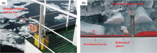
When the R/V Xuelong icebreaker navigated within the ice zone, broken floes were observed to turn over along the hull of the ship with cross sections exposed above the sea surface. Thus, another downward-oriented video camera was fixed onto the portside of the first deck to measure ice thickness levels throughout the cruise (Figure 2(b)). The video camera in this case was set 6.5 m above the sea surface and 0.7 m away from the hull, while to determine the real thickness of the cross section, a plastic sphere with a diameter of 0.4 m was hung along the hull of ship as a reference, set close to the waterline to reduce potential error due to its distance to the ice cross section. This system was run continuously between 2 August 2014 and 1 September 2014, except for the period of LIC.

2.2. Shipborne imagery and analysis

2.2.1. Sea ice thickness

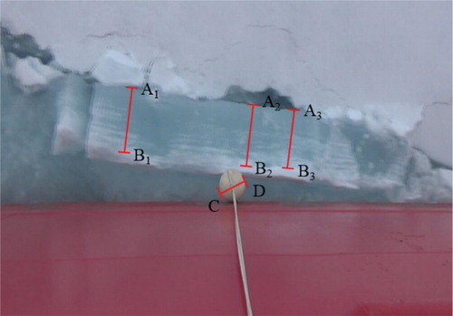
To derive SIT information from downward-oriented shipborne video, image frames containing the whole cross section of overturned level sea ice were initially captured artificially (Figure 3). However, in order to avoid oblique distortion, this cross section needs to be oriented parallel to the image plane. As most floes were covered with a layer of snow, the next step of this analysis was to distinguish the interface between ice and snow on the cross section and obtain SIT pixels within the frame (e.g. A₁B₁, A₂B₂, and A₃B₃). Three in frame thicknesses pixels were extracted for one floe, and the actual SIT of level ice can be determined, as follows:(1) $\text{SIT}=\frac{1}{3}\sum _{j=1}^3{\text{A}}_j{\text{B}}_j\cdot \frac{d}{\text{CD}},$(1) where A_jB_j denotes the SIT pixels in the frame, while CD is the pixels of the diameter of referenced sphere in the frame, and d is the real diameter of referenced sphere. The Coordinated Universal Time of each frame was determined using the video recording time as well as the duration of each frame. Thus, the frame location can be obtained by matching its Coordinated Universal Time with the voyage data recorder. We collected a total of 2459 frames over the whole cruise including 1879 during the northward leg and 580 during the southward section.

Figure 3. One frame containing a whole overturned level ice cross section captured from shipborne video. In this image, A₁B₁, A₂B₂, and A₃B₃ are ice thicknesses in cross section and CD is the diameter of referenced sphere within the frame.

2.2.2. Sea ice concentration

The process of deriving SIC from oblique-oriented pictures included two steps: image partition and correction of geometric distortion. During the first step, the sea surface components were partitioned into three categories: sea ice, melt pond, and open water, by manually selecting red, green, and blue (RGB) thresholds based on the color distribution histograms within each image (Perovich, Tucker , and Ligett 2002; Inoue, Curry, and Maslanik 2008; Lu et al. 2010; Huang et al. 2016; Li et al. 2017). The threshold levels for each surface category in each image were independently determined. The RGB thresholds for each category were assumed to be disparate and that there would be no overlap between threshold levels. Melt ponds can be distinguished from surrounding ice because they look bluish and pond reflectance is greater in the blue portion of the spectrum than in the red (Grenfell and Maykut 1977). Similarly, open water can be identified by its darker appearance because of lower reflectance. Based on these criteria, melt ponds, open water, and sea ice can be separated from each other.

A number of other special cases also warrant discussion including completely developed melt ponds that penetrate throughout the ice, such as melt holes. These were characterized as open water because of their similar optical features. While edge erosion caused by lateral melt was treated as melt pond because of a similar RGB distribution. Finally, new ice layers floating on open water were classified in the same category as they contribute little to surface reflectance because of their negligible thicknesses (Lu et al. 2010; Huang et al. 2016; Li et al. 2017). The accuracy of the classification method has been inspected by Li et al. (2017) using a confusion matrix. They randomly selected 7% photos from the image archive and referred visual interpretation results as the ‘true value’. The Kappa coefficient was more than 0.8, which confirmed the feasibility of the method. We used the same method as Li et al. (2017) in this study and obtained a similar Kappa coefficient, which verified the accuracy of the partitioning method in this study.

It is noteworthy that image planes inclined relative to the sea surface will yield a geometric distortion, which led Hall, Hughes, and Wadhams (2002) to underestimate SIC from uncorrected oblique-oriented photos. During the second step of the process of oblique-oriented image, a method for geometric correction developed by Lu and Li (2010) was applied in this study to correct the geometric distortion of oblique photos and to determine the SIC from calculations of the actual size of the area of each surface component. Besides, this approach could reduce errors caused by ship sway and shadowing by setting an upper limit of the view angle. The area fractions of open water, melt pond, and sea ice were therefore presented as A_w, A_p, and A_i, respectively; it is clear that A_w + A_p+ A_i= 1, and that SIC is the sum of A_p and A_i.

A total of 47,050 oblique-oriented pictures were obtained throughout the whole cruise. Because the visibility was often limited due to heavy fog in Arctic summer, all these images were screened at first. Approximately 15% of them were unable to be processed due to poor contrast under fog condition. Afterwards we selected two pictures for both sides at intervals of 1 h to reduce the enormous workload necessary to select RGB thresholds in each case (Huang et al. 2016). Thus, a final total of 892 pictures from cameras on both sides were used in this study; if two pictures were available for the same location from both sides, then an average was used for the location value.

2.3. Satellite data

Daily SSM/I-SSMIS NT SIC data with a grid resolution of 25 km (at 19 and 37 GHz), processed by the National Snow and Ice Data Center (Cavalieri et al. 1996), and daily AMSR2 SICCI SIC data with a grid resolution of 25 km (at 19 and 37 GHz), processed by the University of Hamburg (Pedersen et al. 2017), were acquired for the same duration as the CHINARE-2014 cruise. The SSM/I and SSMIS instruments were launched onboard the Defense Meteorological Satellite Program satellites and AMSR2 sensor was launched onboard Global Change Observation Mission 1st-Water satellite. All of these satellites orbit the earth in a sun-synchronous circle and cover the polar region every day. Brightness temperatures are recorded by these satellite sensors and the NT SIC and SICCI SIC are retrieved based on the brightness temperature polarization difference (Comiso et al. 1997; Ivanova et al. 2015).

3. Results

3.1. General sea ice conditions

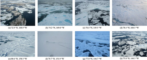
Arctic sea ice conditions at different locations along the cruise exhibit large spatial variations due to the summer melt. At the outer edge of the MIZ, sea ice presented mainly as small crushed ice floating on open water alongside dirty ice from nearshore regions (Figure 4(a)). Melt ponds with bright appearance in blue spread onto the ice surface in distinct shapes (Figure 4(b)). As the ice underneath the pond gets thinner, the pond albedo decreases and the ponds appear darker (Perovich et al. 2009). Therefore those ponds with bright turquoise appearances had enough thickness in underlying ice, while floe size increased and dirty ice disappeared at the outer boundary of the PIZ. At the same time, melt ponds connected with each other and developed into complex networks (Figure 4(c)). Some of ponds even had a very dark appearance due to the fact that these ponds had melt through to the ocean and therefore were referred to as melt holes. At higher latitudes beyond 78°N, small floes or open water were scarcely present, and huge floes covered almost the entire sea surface with ponds spreading on surface (Figure 4(d–f)). In these regions the ice surface seemed smoother because it was covered with a thick snow layer, while during the southward cruise, melt ponds with bright turquoise appearance were rarely seen and they mostly showed dark appearances in irregular shape and developed into networks due to mature evolution (Figure 4(g)). Open water reappeared with small ice floating on it when returning to the outer edge of PIZ (Figure 4(h)), while new ice layers formed on the surfaces of ponds and open water because of early freeze-up.

Figure 4. Typical oblique-oriented photos of ice conditions during the cruise; (a–e) are from the northward cruise while (f–,g) are from the southward.

3.2. SIT along vessel cruise

The distribution of SIT derived from downward-oriented video throughout the cruise is shown in Figure 5. Most of the discontinuities in these data are indicative of open water in the video view, except for the discontinuity at 81°N because of the LIC. During northward cruise in the MIZ, SIT showed large spatial variability with an average of 88.3 ± 28.2 cm, similar to SIT detected using EM31 during the same cruise (92.0 ± 31.0 cm) (Lei et al. 2017). The thinnest recorded floe in MIZ was 23.4 cm while the thickest was 165.1 cm. Data show that as the vessel entered the PIZ during northward cruise, SIT increased rapidly up to more than 100.0 cm, and to more than 120.0 cm in the region north of 78°N. At the same time, SIT varied around an average of 109.3 ± 26.2 cm in the PIZ during northward cruise; as the vessel moved southward within the PIZ from the LIC, SIT thickness decreased gradually to around 100.0 cm, but remained at an average of 110.9 ± 30.3 cm. This similarity in average SIT in the PIZ during both northward and southward section of the cruise indicates small temporal variability over the study duration. Results show that the overall average SIT in the PIZ was 21.5 cm more than that in the MIZ (109.8 ± 27.5 cm versus 88.3 ± 28.2 cm).

Figure 5. The distribution of sea ice thickness along the cruise (black line). The discontinuity in this figure denotes open water or the duration of the long-term ice camp in the northernmost region.

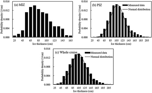
The cruise was divided into two sections, south of 76°N (MIZ) and north of 76°N (PIZ), to characterize the SIT distribution. In the MIZ, SIT varied between 20 and 170 cm with that between 50 and 110 cm encompassing 72% of the thickness distribution (Figure 6(a)). The probability density of SIT in the PIZ was considered to be close to a normal distribution around an average of 109.8 cm and with a standard deviation of 27.5 cm, compared with the normal distribution fitting curve using the observed data (Figure 6(b)), although it was rejected by a KS-test. Thus, SIT between 82.3 and 137.3 cm occupied the dominant portion (68%) of the distribution within the PIZ. While distinct modes could be identified between the PIZ and the MIZ (105 cm versus 75 cm) that are related to large spatial variation. Over the entire cruise, the average SIT was 104.9 ± 29.1 cm with a mode of 105 cm. The SIT probability density also approximatively conformed to a normal distribution with the dominant portion between 75.8 and 134.0 cm compared with the normal distribution fitting curve in spite of a rejection of KS-test (Figure 6(c)).

Figure 6. The probability density of sea ice thickness in the regions of (a) MIZ, (b) PIZ, and (c) the whole cruise. As shown are the normal distribution curves fitting the sea ice thickness distribution in the PIZ and the whole cruise.

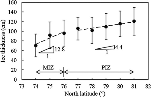
According to spatial variations, the average SIT over the whole cruise at each latitude was plotted (Figure 7) to determine the correlation of SIT with latitude. The results show that mean SIT at the outer edge of the MIZ was 70.4 ± 23.5 cm, rising to 96.1 ± 27.2 cm in the inner MIZ, a gradient of increase of 12.8 (cm/°). Mean SIT at the outer boundary of the PIZ was 105.6 ± 26.3 cm, followed by a slight decline to 101.8 ± 29 cm at 78°N. Subsequently, SIT increased linearly with north latitudes. While SIT showed a varying gradient of 4.4 (cm/°) in the PIZ, about three times less than that in the MIZ, indicative of relatively slower variation.

Figure 7. Average sea ice thicknesses at each latitude and standard deviations along the cruise. Also shown are the regression lines (dash lines) and varying gradients in MIZ and PIZ.

3.3. Sea ice morphology along cruise

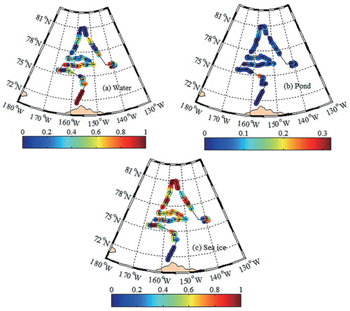
Area fractions were defined as the area ratio of open water, melt pond, and sea ice relative to the observed sea surface, substituted as A_w, A_p, and A_i, respectively, and variations of the area fractions along the cruise are presented in Figure 8. Observations show that there was an offshore ice-free (A_w= 1) region below 73°N near Barrow; as sailing northward into the MIZ, A_w and A_i fluctuated over a wide range, from almost 0 to 1.0, corresponding to averages of 0.52 ± 0.33 and 0.44 ± 0.30, respectively. The large scope of these fluctuations as well as their standard deviations reflect the alternate appearance of open water and sea ice. Observations also show that, A_w decreased and A_i increased rapidly after entering the PIZ, reaching averages of 0.01 ± 0.03 and 0.96 ± 0.07 during LIC for A_w and A_i, respectively. As the vessel returned to 76°N, A_w gradually increased to 1.0 and A_i decreased gradually to 0. Mean A_w and A_i values for the PIZ during the southward cruise were 0.23 ± 0.29 and 0.74 ± 0.28, respectively, similar to those for PIZ during the northward cruise, 0.23 ± 0.25 and 0.72 ± 0.24. These values are indicative of a small temporal variation in sea surface components over the study duration. However, A_p throughout the whole cruise varied within a narrow range, between 0 and 0.32, corresponding to an average of 0.04 ± 0.05.

Figure 8. Variations of the area fractions of (a) water, (b) pond, and (c) sea ice along the cruise (black line) obtained from the oblique photography of sea ice onboard R/V Xuelong.

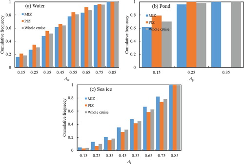
In order to describe variations in sea surface components, frequencies of fractional coverage were analyzed in the MIZ and PIZ. Extreme sections within the frequency (i.e. between 0 and 0.1 and between 0.9 and 1.0 for water and sea ice and between 0 and 0.1 for melt pond) were abandoned for analysis, and results are shown in Figure 9. The results show that in the MIZ, the varying gradient of cumulative frequency of A_w decreased, indicating that the frequency of A_w decreased with increasing A_w. Similarly, as A_p increased from 0.10 to 0.40, the frequency decreased linearly from 0.6 to almost 0, while the frequency of A_i conformed to an opposite trend as the varying trend of their cumulative frequency increased with increasing area fraction. In the PIZ, the cumulative frequency distributions of fractional coverage followed a similar trend to that seen in the MIZ. And considering area fractions from the whole cruise, frequency distributions reveal no obvious differences compared with divided regimes.

Figure 9. Cumulative frequency distributions of the area fractions of (a) water, (b) pond, and (c) sea ice in MIZ, PIZ, and throughout the whole cruise when extreme regions (i.e. between 0 and 0.1 and between 0.9 and 1.0 for water and sea ice, respectively, and between 0 and 0.1 for melt pond) were abandoned.

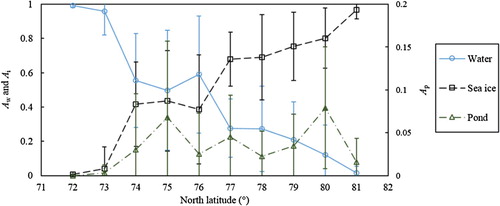
In order to account for changes in ice conditions with latitudes, the mean fractional coverage of surface components at each latitude was shown in Figure 10. Data show that mean A_i was close to 0 at the southern edge of the MIZ, increased to 0.42 ± 0.25 at 74°N, and was maintained around 0.41 within the MIZ. However, after entering the PIZ, mean A_i jumped to 0.68 ± 0.16 at 77°N before increasing with a gradient of 0.07 (/°) between 77°N and 81°N. Average A_w varied in the opposite way against A_i, with an average decrease rate of 0.07(/°) within the PIZ. A_w was higher than A_i below 76°N but this reversed when entering into the PIZ above 76°N. Overall, mean A_p remained very small, less than 0.08. A significant correlation between melt pond fractions and north latitudes was not clear.

Figure 10. Average area fractions and standard deviations of water, pond, and sea ice.

4. Discussions

4.1. Uncertainty assessment of image processing

There are three possible uncertainties contained in the retrievals of SIC. First, the light conditions are changing when capturing oblique images of the sea surface. For example, photographs taken at different time during a day could show discrepant appearance color on melt ponds. Even in the same image, the melt ponds might show different appearance in color due to distinct viewing angle. Thus, some pond-like objects might be mistaken as melt pond. When handling this issue, the manual interaction would eliminate this error. The boundary of melt pond based on the threshold calculated by computer was justified by naked-eyes. Then the objects mistaken as melt ponds, which, actually, were not melt ponds, but brash ice and something else similar to melt ponds were excluded and corrected manually. Second, those melt ponds with very thin underlying ice (less than a few centimeters) often show very dark appearances which resemble melt holes. There is uncertainty, however, in determining whether the very darker melt ponds have melted through to the ocean from the surface appearances in an image. They were classified into melt holes in this study, which indicates that there were an overestimate in open water fraction and an underestimate in melt pond fraction based on our portioning criteria. Finally, weather conditions, especially fogs, largely impacted the image quality. Because ordinary optical cameras were used in the survey and their waveband was just a little wider than visible spectrum. They had limited ability to penetrate through fogs. Those images with poor contrast had to be deleted. An infrared camera which has a higher penetrating ability may be helpful in the future observation to overcome the weather impact and improve the quality of data.

4.2. A comparison of SIC from shipborne images with that from satellite data

Because the distances between the locations of two adjoining images were more than 20 km in nearly half of the photos, covering several grids of satellite products with higher resolution, data from AMSR2 SICCI SIC (25 km) and SSM/I-SSMIS NT SIC (25 km) are presented as comparisons for shipborne observations. The fixed grid of satellite data might not correspond to the locations of shipborne images. Thus, SIC recorded by each satellite on the same day as shipborne observation was interpolated to each oblique-oriented photo location using the value of the closest grid point. When the displacement between the locations of two adjoining images was less than the satellite resolution, shipborne SIC was smoothed by a moving average to fit to the satellite resolution. Therefore, the SIC from different sources with distinct resolutions could be compared.

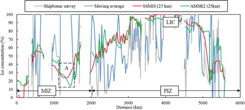
The results in Figure 11 show that shipborne SIC and the moving average fluctuated irregularly when cruising through the MIZ, indicating a frequently alternation between sea ice and open water. After entering the PIZ, both shipborne SIC and moving average gradually increased to 100% while sailing northwards to the LIC. But when the vessel turned back, both shipborne SIC and moving average dropped rapidly. Satellite-derived SIC exhibited a generally similar trend to shipborne values, except that area A (around 75.5°N, 165.9°W) was recorded by RS as almost ice-free due to coarse resolution even though local scale shipborne observations showed the sea surface was covered with ice.

Figure 11. SIC derived from shipborne observations and its moving average along the cruise route. SIC values from SSMIS (25 km) and AMSR2 (25 km) data are shown for comparison. The MIZ, PIZ, location of the LIC, and a special area A with explanations in context are shown.

In order to validate the accuracy of RS, shipborne SIC values without moving averages were used as a reference criterion (Table 1). Differences between satellites and moving averages across the whole SIC section were 9.5% and 9.9% for SSMIS (25 km) and AMSR2 (25 km), respectively. Although there were a small number of overestimates based on RS, discrepancies changed in areas with very low (<15%) and high (>75%) SIC. In the open water area, overestimation was enhanced in the case of the two satellites, while RS overestimated the SIC moving average by 12% and 16.4% for SSMIS (25 km) and AMSR2 (25 km), respectively. In close ice regions, however, RS underestimated the SIC moving average by 4.4% and 8.9% for SSMIS (25 km) and AMSR2 (25 km), respectively, similar satellite errors to those recovered in other studies (Steffen and Schweiger 1991; Alekseeva and Frolov 2013).

Table 1. Mean sea ice concentration derived from moving averages and RS for different sections.

Shipborne SIC (%)	Moving average (%)	SSMIS (25 km) (%)	AMSR2 (25 km) (%)
0–100	63.9 ± 33.8	73.4 ± 30.0	73.8 ± 25.0
≤15	43.6 ± 85.8	55.6 ± 92.6	60.0 ± 91.6
≥75	93.3 ± 9.3	88.9 ± 20.0	84.4 ± 18.2

Certainly, there were uncertainties in the comparison between RS SIC and moving average SIC. First of all, the moving average of shipborne SIC could probably cover the satellite footprint in the dimension along the ship track. However, it could not correspond to satellite resolution in the dimension across the track because the observing area of shipborne oblique images was a narrow strip. During the comparisons, we assumed isotropic ice conditions, i.e. that ship data was taken representative for RS pixels as Lu and Li (2010). Second, RS SIC are daily averages, in contrast, shipborne SIC are instantaneously obtained. Ice conditions at any location could change because sea ice is always drifting. Whereas, considering the drift speed of sea ice (Martin and Augstein 2000; Sumata et al. 2015), the sea ice which is captured in the shipborne observing area could not drift out of the region of the pixel resolution (25 km × 25 km). Therefore, the effect temporal asynchrony between shipborne SIC and RS data on the accuracy of the comparison could be neglected.

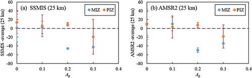
Melt ponds affect the accuracy of SIC derived from satellites (Ivanova et al. 2015; Kern et al. 2016). To detect the possible impact of melt ponds on satellite-derived SIC, difference variations between RS and shipborne observation with A_p are shown in Figure 12. One common trend revealed by these data is that RS data are inclined to underestimate SIC at increasing pond fractions; for example, in the MIZ, when A_p was below 0.1, SIC derived from satellites and shipborne observations were close to one another (<±10%), while when A_p increased above 0.2, these differences dropped below −35%, significant underestimations. However, in the PIZ, satellites overestimated SIC by between 3.2% and 13.6% when A_p was below 0.2, and underestimated SIC by about 19% when A_p= 0.3. Such underestimations at high A_p were probably the result of the almost full development of melt ponds; these ponds, although they did not penetrate the underlying ice, were nevertheless identified as water due to their dark appearance.

Figure 12. The impact of A_p on differences between satellite-derived and shipborne sea ice concentration for (a) SSMIS (25 km) and (b) AMSR2 (25 km) in the MIZ and PIZ.

4.3. Areal surface albedo

Large spatial discrepancies in sea surface morphology lead to changes in composite surface albedo, which has a considerable impact on solar energy reflectance. The surface albedo can be determined using the image-derived area fractions by weighing the albedos of sea surface components by their fractional coverage as followed equation:(2) $\overline{\alpha }={\alpha }_{\mathrm{i}}{A}_{\mathrm{i}}+{\alpha }_{\mathrm{p}}{A}_{\mathrm{p}}+{\alpha }_{\mathrm{w}}{A}_{\mathrm{w}},$(2) where $\overline{\alpha }$ refers to composite surface albedo, while α_i, α_p, and α_w denote the broadband albedos of sea ice, melt pond, and open water, respectively. This expression has been employed in many previous studies (Tschudi, Curry, and Maslanik 2001; Perovich et al. 2009; Lu et al. 2010; Li et al. 2017) to estimate area albedo. Besides, comparisons of the calculated albedo with field measurements have been conducted in Lu et al. (2010) to validate the feasibility of the method.

Although area fractions are obtained based on visible spectrum, the albedo of each sea surface component was set based on broadband spectrum. Thus $\overline{\alpha }$ in Equation (2) is the broadband area albedo. Arctic sea ice is often covered by snow, so a range between 0.55 and 0.80 was used for α_i, corresponding to the fluctuating value between bare ice and snow-covered ice (Grenfell and Perovich 2004; Hudson et al. 2013). In addition, α_p is known to vary in both space and time because of its sensitivity to pond depth and underlying ice thickness (Lu et al. 2016a); thus, a range between 0.15 and 0.34, the threshold albedos of two typical ponds (dark pond and bright pond), was assigned based on the observation that the developing stage of ponds are associated with surface appearance (Hudson et al. 2013). Finally, α_w was set at 0.07 due to limited variability (Pegan and Paulson 2001; Lu et al. 2010). An estimated area albedo from Perovich et al. (2009) was used here to check the albedo calculated in this study. With an ice condition of A_w = 0.07, A_p = 0.29, and A_i = 0.64, they gave an estimated surface albedo value of 0.49. Putting the area fractions into Equation (2), the albedo range was 0.40–0.62 with an average of 0.51, which agreed well with the value in Perovich et al. (2009), confirming the feasibility of our method.

The composite broadband surface albedo at each latitude was calculated by inputting average area fractions (Figure 10), and the results of these calculations are shown in Figure 13. Data show that mean surface albedo varied between 0.07 and 0.66 and was significantly associated with latitude, showing a large spatial variations. At latitudes below 73°N, mean surface albedos were less than 0.10, while within the MIZ, values reached an average of 0.33, a saltation above 0.20 compared with lower latitudes. Subsequent to entering the PIZ, surface albedo values increased more, conforming to a gradient of 0.04(/°) with north latitudes between 77°N and 81°N.

Figure 13. Maximum, average, and minimum broadband surface albedos at each latitude calculated using image-derived average area fractions during the CHINARE-2014 cruise. Surface albedos from other cruises (SHEBA, CHINARE-2008 and CHINARE-2010) are shown for comparison.

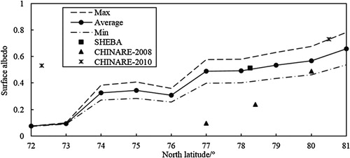
A number of other cruises have also measured broadband surface albedo over the same season in this region, including the Surface Heat Budget of the Arctic Ocean (SHEBA) (Perovich, Tucker , and Ligett 2002), CHINARE-2008 (Lu et al. 2010), and CHINARE-2010 (Xie et al. 2013, 2015); the results of these expeditions are also plotted in Figure 13 for comparison. Comparing matching latitudes, the surface albedo observed by SHEBA (22 August 1998) is similar to that recorded in this cruise, while the surface albedos reported by CHINARE-2008 at 77°N (5 September 2008), 78.4°N (4 September 2008), and 78°N (17 August 2008) were 5.1, 2.1, and 1.2 times lower than those reported here, respectively. One likely reason for these differences is that the SIC in 2008 was small, just 3%, 12%, and 52% at 77°N, 78.4°N, and 80°N, respectively. However, the surface albedos measured by CHINARE-2010 at 72.3°N (27 July 2010) and at 80.5°N (1 August 2010) were 7.0 and 1.3 times higher than those reported here, also likely the result of interannual SIC variation (72% at 72.3°N and 100% at 80.5°N in 2010).

5. Conclusions

Sea ice conditions were observed continuously throughout the CHINARE-2014 cruise in the Pacific Arctic sector. A video mounted face-down as well as two cameras mounted obliquely were used to capture level sea ice turnover as well as the sea surface morphology. Observations show that sea ice conditions exhibited large spatial and relatively small temporal variations throughout the duration of the expedition and the whole ice region could be divided into MIZ and PIZ based on the boundary of 76°N. Mean SIT was 88.8 ± 28.2 cm in the MIZ and 109.3 ± 26.2 cm in the PIZ. At the same time, mean A_w and A_i were 0.52 ± 0.33 and 0.44 ± 0.30 within MIZ, respectively, and were 0.23 ± 0.29 and 0.74 ± 0.28 within the PIZ, while mean A_p was 0.04 ± 0.05 throughout the whole cruise. Compared with ice conditions in a similar domain and over a similar duration during the CHINARE-2010 cruise (Xie et al. 2013), the outer ice edge recorded here was about 2.2° backwards, mean SIT was 20.5 cm less, and mean SIC was 5.6% less.

SSMIS (25 km) and AMSR2 (25 km) satellite data overestimated the SIC by 9.5% and 9.9% compared with shipborne measurements. However, for areas with SIC less than 15%, this overestimation increased to 12% and 16.4% for SSMIS (25 km) and AMSR2 (25 km) data, while underestimating by 4.4% and 8.9% in areas with SIC more than 75%, respectively. A common trend was found for both satellite sensors that they are inclined to underestimate the SIC with increasing pond fractions.

The average areal surface albedo determined based on shipborne SIC increased northward from 0.07 to 0.66, significantly correlated with the SIC spatial variation; data show an average of 0.23 and an increase of 0.07 (/°) in the MIZ and an average of 0.55 and an increase of 0.04 (/°) in the PIZ. Surface albedos from previous campaigns in similar regions over similar durations were compared and reveal a range of results, likely due to rapid interannual variation in summer SIC.

Arctic sea ice is changing rapidly, and further accumulation of ice conditions will be required for Arctic navigations. As the R/V Xuelong tended to sail through a region with less ice during the cruise, the data collected in this study will prove useful for future commercial navigations and to validate satellite data. In order to provide more ground truth data with higher coverage, helicopter or unmanned aerial vehicle survey coordinated with shipborne investigations would be helpful in the future. An infrared camera is also necessary to overcome the bad atmospheric conditions.

Disclosure statement

No potential conflict of interest was reported by the authors.

Additional information

Funding

This work was supported by the National Key Research and Development Program of China [grant number 2016YFC1402702], [grant number 2015CB953901]; the National Natural Science Foundation of China [grant number 41676187], [grant number 41428603], [grant number 41376186], [grant number 41722605]; the High Technology of Ship Research Project of the Ministry of Industry and Information Technology [grant number [2013]417], [grant number [2013]412]; and Academy of Finland [grant number 283101].

References

- Alekseeva, T. A., and S. V. Frolov. 2013. “Comparative Analysis of Satellite and Shipborne Data on Ice Cover in the Russian Arctic Seas.” Izvestiya, Atmospheric and Oceanic Physics 49: 879–885. doi:10.1134/s000143381309017x.
- Beitsch, A., S. Kern, and L. Kaleschke. 2015. “Comparison of SSM/I and AMSR-E Sea Ice Concentrations with ASPeCt Ship Observations Around Antarctica.” IEEE Transactions on Geoscience and Remote Sensing 53: 1985–1996. doi:10.1109/TGRS.2014.2351497.
- Cavalieri, D., C. Parkinson, P. Gloersen, and H. J. Zwally. 1996. Sea Ice Concentrations From Nimbus-7 SMMR and DMSP SSM/I-SSMIS Passive Microwave Data, Version 1. [Indicate Subset Used] , updated yearly. Boulder, CO: NASA DAAC at the National Snow and Ice Data Center.
- Comiso, J. C. 2012. “Large Decadal Decline of the Arctic Multiyear Ice Cover.” Journal of Climate 25: 1176–1193. doi:10.1175/JCLI-D-11-00113.1.
- Comiso, J. C., D. J. Cavalieri, C. L. Parkinson, and P. Gloersen. 1997. “Passive Microwave Algorithms for Sea Ice Concentration: A Comparison of Two Techniques.” Remote Sensing of Environment 60: 357–384. doi:10.1016/S0034-4257(96)00220-9.
- Comiso, J. C., C. L. Parkinson, R. Gersten, and L. Stock. 2008. “Accelerated Decline in the Arctic Sea Ice Cover.” Geophysical Research Letters 35: L01703. doi:10.1029/2007gl031972.
- Grenfell, T. C., and G. A. Maykut. 1977. “The Optical Properties of Ice and Snow in the Arctic Basin.” Journal of Glaciology 18: 445–463. doi:10.1017/S0022143000021122.
- Grenfell, T. C., and D. K. Perovich. 2004. “Seasonal and Spatial Evolution of Albedo in a Snow-ice-land-ocean Environment.” Journal of Geophysical Research 109: C01001. doi:10.1029/2003jc001866.
- Haas, C., J. Lobach, S. Hendricks, L. Rabenstein, and A. Pfaffling. 2009. “Helicopter-borne Measurements of Sea Ice Thickness, Using a Small and Lightweight, Digital EM System.” Journal of Applied Geophysics 67: 234–241. doi:10.1016/j.jappgeo.2008.05.005.
- Hall, R. J., N. Hughes, and P. Wadhams. 2002. “A Systematic Method of Obtaining Ice Concentration Measurements from Ship-based Observations.” Cold Regions Science and Technology 34: 97–102. doi:10.1016/S0165-232X(01)00057-X.
- Huang, W., P. Lu, R. Lei, H. Xie, and Z. Li. 2016. “Melt Pond Distribution and Geometry in High Arctic Sea Ice Derived from Aerial Investigations.” Annals of Glaciology 57: 105–118. doi:10.1017/aog.2016.30.
- Hudson, S. R., M. A. Granskog, A. Sundfjord, A. Randelhoff, A. H. H. Renner, and D. V. Divine. 2013. “Energy Budget of First-year Arctic Sea Ice in Advanced Stages of Melt.” Geophysical Research Letters 40: 2679–2683. doi:10.1002/grl.50517.
- Inoue, J., J. A. Curry, and J. A. Maslanik. 2008. “Application of Aerosondes to Melt-pond Observations Over Arctic Sea Ice.” Journal of Atmospheric and Oceanic Technology 25: 327–334. doi:10.1175/2007JTECHA955.1.
- Istomina, L., G. Heygster, M. Huntemann, P. Schwarz, G. Birnbaum, R. Scharien, C. Polashenski, et al. 2015. “Melt Pond Fraction and Spectral Sea Ice Albedo Retrieval from MERIS Data − Part 1: Validation Against In Situ, Aerial, and Ship Cruise Data.” The Cryosphere 9: 1551–1566. doi:10.5194/tc-9-1551-2015.
- Ivanova, N., O. M. Johannessen, L. T. Pedersen, and R. T. Tonboe. 2014. “Retrieval of Arctic Sea Ice Parameters by Satellite Passive Microwave Sensors: A Comparison of Eleven Sea Ice Concentration Algorithms.” IEEE Transactions on Geoscience and Remote Sensing 52: 7233–7246. doi:10.1109/TGRS.2014.2310136.
- Ivanova, N., L. T. Pedersen, R. T. Tonboe, S. Kern, G. Heygster, T. Lavergne, A. Sørensen, et al. 2015. “Inter-comparison and Evaluation of Sea Ice Algorithms: Towards Further Identification of Challenges and Optimal Approach Using Passive Microwave Observations.” The Cryosphere 9: 1797–1817. doi:10.5194/tc-9-1797-2015.
- Kern, S., A. Rösel, L. T. Pedersen, N. Ivanova, R. Saldo, and R. T. Tonboe. 2016. “The Impact of Melt Ponds on Summertime Microwave Brightness Temperatures and Sea Ice Concentrations.” The Cryosphere 10: 2217–2239. doi:10.5194/tc-10-2217-2016.
- Khon, V. C., and I. I. Mokhov. 2010. “Arctic Climate Changes and Possible Conditions of Arctic Navigation in the 21st Century.” Izvestiya, Atmospheric and Oceanic Physics 46: 14–20. doi:10.1134/s0001433810010032.
- Knuth, M. A., and S. F. Ackley. 2006. “Summer and Early-fall Sea-ice Concentration in the Ross Sea: Comparison of In Situ ASPeCt Observations and Satellite Passive Microwave Estimates.” Annals of Glaciology 44: 303–309. doi:10.3189/172756406781811466.
- Kurtz, N. T., T. Markus, D. J. Cavalieri, W. Krabill, J. G. Sonntag, and J. Miller. 2008. “Comparison of ICESat Data With Airborne Laser Altimeter Measurements Over Arctic Sea Ice.” IEEE Transactions on Geoscience and Remote Sensing 46: 1913–1924. doi:10.1109/TGRS.2008.916639.
- Kwok, R., and G. F. Cunningham. 2010. “Contribution of Melt in the Beaufort Sea to the Decline in Arctic Multiyear Sea Ice Coverage: 1993−2009.” Geophysical Research Letters 37: 79–93. doi:10.1029/2010gl044678.
- Lei, R., Z. Li, N. Li, P. Lu, and B. Cheng. 2012. “Crucial Physical Characteristics of Sea Ice in the Arctic Section of 143°−180°W During August and Early September 2008.” Acta Oceanologica Sinica 31: 65–75. doi:10.1007/s13131-012-0221-0.
- Lei, R., X. Tian-Kunze, B. Li, P. Heil, J. Wang, J. Zeng, and Z. Tian. 2017. “Characterization of Summer Arctic Sea Ice Morphology in the 135°−175°W Sector Using Multi-scale Methods.” Cold Regions Science and Technology 133: 108–120. doi:10.1016/j.coldregions.2016.10.009.
- Li, L., C. Ke, H. Xie, R. Lei, and A. Tao. 2017. “Aerial Observations of Sea Ice and Melt Ponds Near the North Pole During CHINARE2010.” Acta Oceanologica Sinica 36: 64–72. doi:10.1007/s13131-017-0994-2.
- Lindsay, R., and A. Schweiger. 2015. “Arctic Sea Ice Thickness Loss Determined Using Subsurface, Aircraft, and Satellite Observations.” The Cryosphere 9: 269–283. doi:10.5194/tc-9-269-2015.
- Liu, M., and J. Kronbak. 2010. “The Potential Economic Viability of Using the Northern Sea Route (NSR) as an Alternative Route Between Asia and Europe.” Journal of Transport Geography 18: 434–444. doi:10.1016/j.jtrangeo.2009.08.004.
- Lu, P., M. Leppäranta, B. Cheng, and Z. Li. 2016a. “Influence of Melt-pond Depth and Ice Thickness on Arctic Sea-ice Albedo and Light Transmittance.” Cold Regions Science and Technology 124: 1–10. doi:10.1016/j.coldregions.2015.12.010.
- Lu, P., and Z. Li. 2010. “A Method of Obtaining Ice Concentration and Floe Size from Shipboard Oblique Sea Ice Images.” IEEE Transactions on Geoscience and Remote Sensing 48: 2771–2780. doi:10.1109/TGRS.2010.2042962.
- Lu, P., Z. Li, B. Cheng, R. Lei, and R. Zhang. 2010. “Sea Ice Surface Features in Arctic Summer 2008: Aerial Observations.” Remote Sensing of Environment 114: 693–699. doi:10.1016/j.rse.2009.11.009.
- Lu, W., Q. Zhang, R. Lubbad, S. Løset, and R. Skjetne. 2016b. “A Shipborne Measurement System to Acquire Sea Ice Thickness and Concentration at Engineering Scale.” Paper presented at Arctic Technology Conference, Newfoundland and Labrador, October 24−26.
- Martin, T., and E. Augstein. 2000. “Large-scale Drift of Arctic Sea Ice Retrieved From Passive Microwave Satellite Data.” Journal of Geophysical Research 105: 8775–8788. doi:10.1029/1999JC900270.
- Miao, X., H. Xie, S. F. Ackley, D. K. Perovich, and C. Ke. 2015. “Object-based Detection of Arctic Sea Ice and Melt Ponds Using High Spatial Resolution Aerial Photographs.” Cold Regions Science and Technology 119: 211–222. doi:10.1016/j.coldregions.2015.06.014.
- Overgaard, S., P. Wadhams, and M. Leppäranta. 1983. “Ice Properties in the Greenland and Barents Seas During Summer.” Journal of Glaciology 29: 142–164. doi:10.1017/S0022143000005219.
- Pedersen, L. T., G. Dybkjær, S. Eastwood, G. Heygster, N. Ivanova, S. Kern, T. Lavergne, et al. 2017. ESA Sea Ice Climate Change Initiative (Sea_Ice_cci): Sea Ice Concentration Climate Data Record from the AMSR-E and AMSR-2 Instruments at 25km Grid Spacing, Version 2.0. Centre for Environmental Data Analysis. doi:10.5285/c61bfe88-873b-44d8-9b0e-6a0ee884ad95.
- Pegan, W. S., and C. A. Paulson. 2001. “The Albedo of Arctic Leads in Summer.” Annals of Glaciology 33: 221–224. doi:10.3189/172756401781818833.
- Perovich, D. K., T. C. Grenfell, B. Light, B. C. Elder, J. Harbeck, C. Polashenski, W. B. Tucker III, et al. 2009. “Transpolar Observations of the Morphological Properties of Arctic Sea Ice.” Journal of Geophysical Research 114: C00A04. doi:10.1029/2008JC004892.
- Perovich, D. K., W. B. Tucker III, and K. A. Ligett. 2002. “Aerial Observations of the Evolution of Ice Surface Conditions During Summer.” Journal of Geophysical Research 107: 8048. doi:10.1029/2000jc000449.
- Renner, A. H. H., S. Gerland, C. Haas, G. Spreen, J. F. Beckers, E. Hansen, M. Nicolaus, and H. Goodwin. 2014. “Evidence of Arctic Sea Ice Thinning from Direct Observations.” Geophysical Research Letters 41: 5029–5036. doi:10.1002/2014gl060369.
- Serreze, M. C., and R. G. Barry. 2011. “Processes and Impacts of Arctic Amplification: A Research Synthesis.” Global and Planetary Change 77: 85–96. doi:10.1016/j.gloplacha.2011.03.004.
- Shibata, H., K. Izumiyama, K. Tateyama, H. Enomoto, and S. Takahashi. 2013. “Sea-ice Coverage Variability on the Northern Sea Routes, 1980−2011.” Annals of Glaciology 54: 139–148. doi:10.3189/2013AoG62A123.
- Spreen, G., L. Kaleschke, and G. Heygster. 2008. “Sea ice Remote Sensing Using AMSR-E 89-GHz Channels.” Journal of Geophysical Research 113: C02S03. doi:10.1029/2005JC003384.
- Steffen, K., and A. Schweiger. 1991. “NASA Team Algorithm for Sea Ice Concentration Retrieval from Defense Meteorological Satellite Program Special Sensor Microwave Imager: Comparison with Landsat Satellite Imagery.” Journal of Geophysical Research 96: 21971–21987. doi:10.1029/91jc02334.
- Stroeve, J. C., V. Kattsov, A. Barrett, M. Serreze, T. Pavlova, M. Holland, and W. N. Meier. 2012. “Trends in Arctic Sea Ice Extent from CMIP5, CMIP3 and Observations.” Geophysical Research Letters 39: L16502. doi:10.1029/2012gl052676.
- Sumata, H., R. Kwok, R. Gerdes, F. Kauker, and M. Karcher. 2015. “Uncertainty of Arctic Summer Ice Drift Assessed by High-resolution SAR Data.” Journal of Geophysical Research 120: 5285–5301. doi:10.1002/2015JC010810.
- Tekeli, A. E., S. Kern, S. F. Ackley, B. Ozsoy-Cicek, and H. Xie. 2011. “Summer Antarctic Sea Ice as Seen by ASAR and AMSR-E and Observed During Two IPY Field Cruises: A Case Study.” Annals of Glaciology 52: 327–336. doi:10.3189/172756411795931697.
- Tschudi, M. A., J. A. Curry, and J. A. Maslanik. 2001. “Airborne Observations of Summertime Surface Features and Their Effect on Surface Albedo During FIRE/SHEBA.” Journal of Geophysical Research 106: 15335–15344. doi:10.1029/2000JD900275.
- Weissling, B., S. Ackley, P. Wagner, and H. Xie. 2009. “EISCAM – Digital Image Acquisition and Processing for Sea Ice Parameters from Ships.” Cold Regions Science and Technology 57: 49–60. doi:10.1016/j.coldregions.2009.01.001.
- Worby, A. P., and I. Allison. 1999. A Technique for Making Ship-based Observations of Antarctic Sea Ice Thickness and Characteristics, Part I: Observational Techniques and Results. Antarctic CRC Research Report 14, 1–23. Hobart, Tasmania. ISBN: 1875796096.
- Worby, A. P., C. A. Geiger, M. J. Paget, M. L. Van Woert, S. F. Ackley, and T. L. DeLiberty. 2008. “Thickness Distribution of Antarctic Sea Ice.” Journal of Geophysical Research 113: C05S92. doi:10.1029/2007jc004254.
- Xia, W., H. Xie, C. Ke, J. Zhao, R. Lei, and S. F. Ackley. 2015. “Summer Surface Albedo of Sea Ice in Pacific Arctic Sector as Measured During the CHINARE 2010 Cruise.” Arctic, Antarctic, and Alpine Research 47: 645–656. doi:10.1657/aaar0014-090.
- Xie, H., R. Lei, C. Ke, H. Wang, Z. Li, J. Zhao, and S. F. Ackley. 2013. “Summer Sea Ice Characteristics and Morphology in the Pacific Arctic Sector as Observed During the CHINARE 2010 Cruise.” The Cryosphere 7: 1057–1072. doi:10.5194/tc-7-1057-2013.
- Zhang, Q., and R. Skjetne. 2015. “Image Processing for Identification of Sea-ice Floes and the Floe Size Distributions.” IEEE Transactions on Geoscience and Remote Sensing 53: 2913–2924. doi:10.1109/TGRS.2014.2366640.