Parameterization of the freeze/thaw discriminant function algorithm using dense in-situ observation network data

ABSTRACT

The near-surface soil freeze–thaw (FT) transition is an important factor affecting land-atmosphere exchanges, hydrology and carbon cycles. Thus, effectively monitoring the temporal–spatial changes of soil FT processes is crucial to climate change and environment research. Several approaches have been developed to detect the soil FT state from satellite observations. The discriminant function algorithm (DFA) uses temperature and emissivity information from Advanced Microwave Scanning Radiometer Enhanced (AMSR-E) passive microwave satellite observations. Although it is well validated, it was shown to be insufficiently robust for all land conditions. In this study, we use in-situ observed soil temperature and AMSR-E brightness temperature to parameterize the DFA for soil FT state detection. We use the in-situ soil temperature records at 5 cm selected from available dense networks in the Northern Hemisphere as a reference. Considering the distinction between ascending and descending orbits, two different sets of parameters were acquired for each frequency pair. The validation results indicate that the overall discriminant accuracy of the new function can reach 90%. We further compared the Advanced Microwave Scanning Radiometer 2 discriminant results using the new function to the Soil Moisture Active Passive freeze/thaw product, and a reasonable consistency between them was found.

KEYWORDS:

• Soil freeze–thaw state
• discriminant function algorithm
• AMSR-E
• AMSR2
• SMAP

1. Introduction

Frozen ground is an important component of the cryosphere, which mainly refers to surface whose temperature is at or below the freezing point and contains ice. Frozen ground can be divided into permafrost, seasonal frozen ground and areas that experience short-term freeze–thaw (FT) cycles. Permafrost is defined as subsurface earth materials that remain below 0° for at least two continuous years (Dobinski 2011), while seasonal frozen ground persists for half month or several months and short-term FT cycles usually lasts only a few hours or days. The distribution of frozen ground is mainly concentrated in the northern hemisphere, where about 24% of land surface is permafrost (Zhang et al. 1999, 2000), and approximately 55% of the exposed land surface of the Northern Hemisphere experienced frozen state. The FT process of land surface is widespread with strong dynamics. About 50 million square kilometres of land surface in the Northern Hemisphere has undergone the process of FT transition every year. The near-surface FT cycles normally occur in the upper layer of permafrost, called the active layer of permafrost (Schuur et al. 2008). The FT state of surface has an important influence on energy exchange, surface runoff, crop growth and carbon cycle (Goodison, Brown, and Grane 1998; Zhang and Armstrong 2001; Zhang, Armstrong, and Smith 2003). In general, the appearance of seasonal thawing and snow melting water is usually consistent with the start time of the plant growing season which is also closely tied to the carbon balance (Oechel et al. 2000; Kimball et al. 2001; Kimball and Mcdonald 2004). In the non-frozen period, with the increase of temperature, the amount of liquid water in the environment increases, the respiration of the soil and the photosynthesis of the vegetation are gradually enhanced (Black et al. 2000) which leads to a substantial increase of the greenhouse gas exchange between the land surface and atmosphere. However, when the frozen period begins, it reduces the water availability in the soil and organisms turn into the dormant period or slow activity period, the exchanges between the land–atmosphere weaken. Since the 1980s, with the global warming of the land surface, the plant’s growth season not only starts earlier than the original time but also becomes longer than the former (Du 2007), which has in turn resulted in an increase in net primary productivity of vegetation (Panneer Selvam et al. 2016). Therefore, monitoring the freezing and thawing process has important theoretical significance and application value for a more comprehensive understanding of land surface process and its response to the influence of human activities. Additionally, the timing and duration of surface FT can be used as a sensitive indicator of climate change (Zhang and Armstrong 2001; Zhang, Armstrong, and Smith 2003). However, these applications require long time series of FT cycles that cover large geographical areas, which are impractical to collect in situ. Satellite-based microwave remoting sensing has proven an efficient way to discriminate FT state due to its all-weather, all-time capabilities, long-wave radiation and sensitive to soil moisture change (Han et al. 2014). Soil FT process is actually the phase change process of liquid water and solid ice in soil. Because of the large difference in dielectric properties between ice and water, the microwave signal (i.e. brightness temperature or backscattering coefficient) substantially change when water freeze, which leads to the basic principle of microwave remote sensing of the surface FT state (Entekhabi et al. 2010; Kim et al. 2011).

In recent years, several FT algorithms based on passive microwave radiation characteristics were developed. It includes dual-indices (Zuerndorfer and England 1992; Zhang, Armstrong, and Smith 2003), new dual-indices (Han et al. 2015), decision tree (Jin, Li, and Che 2009; Jin et al. 2015) and discriminant function algorithm (DFA) (Zhao et al. 2011). There are also FT algorithms based on active microwave information relying on the time change detection. It mainly includes three algorithms which are seasonal threshold method (Rignot and Way 1994; Way et al. 1997; Entekhabi et al. 2004; Gamon et al. 2004), threshold window method (Frolking et al. 1999; Kimball et al. 2001; Kimball, McDonald, et al. 2004; Kimball and Mcdonald 2004; Rawlins et al. 2005) and edge detection method (Canny 1986). Besides, in recent years there has been a great interest in L-band technology such as Soil Moisture and Ocean Salinity (SMOS) and Soil Moisture and Active Passive (SMAP) (Entekhabi et al. 2010; Kerr et al. 2012) due to its sensitivity to soil water phase transition (Rautiainen et al. 2012). Due to the high revisit period of time and many new types of passive microwave sensors, passive microwave remote sensing has huge potential for large-scale FT detection. The DFA was developed based on Advanced Microwave Scanning Radiometer for EOS (AMSR-E) passive microwave imagery (Zhao et al. 2011), where the concepts of ‘quasi-temperature’ and ‘quasi-emissivity’ were used as two criteria to discriminate the FT state. The authors developed the algorithm based on the observed brightness temperature (Tb) from a trunk-mounted microwave radiometer and data simulated by physical models. In another study, the DFA was used to obtain global near-surface FT state validated using the World Meteorological Organization (WMO) weather stations data, Global Land Data Assimilation Systems (GLDAS) modelled soil temperature and the International Soil Moisture Network (ISMN) soil temperature (Hu, Zhao, Shi, Wang, et al. 2016). Despite this progress, the DFA still lacks sufficient calibration and validation on a global scale and as yet does not consider the differences between ascending orbit and descending orbit.

This paper aims to parameterize the FT DFA for different overpassing time. The study aims to refine the performance of the DFA for detecting the near-surface FT state by using AMSR-E observations. The performance of the refined DFA was further tested using imagery from Advanced Microwave Scanning Radiometer 2 (AMSR2) in order to compare with the SMAP freeze/thaw product.

2. Data and methods

2.1. Data sources

2.1.1. Dense in-situ soil temperature measurements

A dense in-situ soil temperature at 5 cm selected from all over the Northern Hemisphere was collected. The Aqua orbit is sun-synchronous with equator crossings at 01:30 pm and 01:30 am local solar time, approximately corresponding to the hottest and coldest time of the day and AMSR-E is one sensor of the satellite. Thus, at each station, data (soil temperature at 5 cm) corresponding to 01:30 pm and 01:30 am were retrieved. However, some stations only have hourly data. To solve this problem, we use the average value of 01:00 and 02:00 to be as the soil temperature of 01:30. Due to the coarse resolution of AMSR-E imagery, a single station generally cannot represent the soil temperature of a single pixel (Roy et al. 2017). In order to better represent the soil temperature within a pixel, only dense in-situ stations whose location is in one AMSR-E pixel were taken. The average value of the soil temperature of these stations was calculated to obtain the soil temperature in the pixel. In addition, considering the difference among different regions, five networks located in China, America, Canada and Finland were selected (Table 1). According to the above, one network contains several pixels and one pixel includes several in-situ single stations.

Table 1. Details of networks.

Network	State	Pixels	Single stations	Row	Column	In-situ observation Points	Points for parameterization
CTP-SMTMN	China	3	3	1087	233	1749	1749
			3	1087	236
			5	1088	234
USA_NET	USA	3	2	304	192	5484	5400
			2	292	170
			2	123	86
FLUXNET	Canada	3	4	302	145	6409	5400
			3	300	145
			4	297	143
FMI	Finland	1	7	827	91	3430	1800
APEX	Alaska (USA)	4	8	127	102	8167	7200
			1	139	105
			1	119	118
			1	120	112

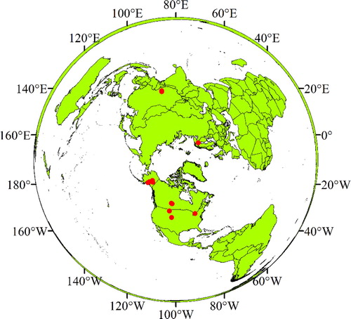
The CTP-SMTMN network which is in a cold semiarid climate in Qinghai-Tibet Plateau in China. Its stations provide in-situ data for three AMSR-E pixels covering the period 1 August 2010 to 27 September 2011. These data can be obtained in the Third Pole Environment Database (http://en.tpedatabase.cn/portal/MetaDataList.jsp). In Canada, three sites were selected: the Met2GF site includes four single stations, the BERMS_OAB site includes three single stations, and the SKfire site includes four single stations each representing one AMSR-E pixel. The data of all selected stations extend from 1 January 2008 to 31 December 2010 and were acquired from FLUXNET Canada Research Network – Canadian Carbon Program Data Collection, 1993–2014 database (https://daac.ornl.gov/cgi-bin/dsviewer.pl?ds_id=1335). The FMI network has one site containing seven single stations which span from 1 January 2007 to 27 September 2011 and was acquired in the LITDB database of the Ground-Based Data Sets of the Arctic Research Centre of Finnish Meteorological Institute (http://litdb.fmi.fi/). The USA_NET network contains three sites whose data can be obtained by the Soil Climate Analysis Network (SCAN) in America (https://www.wcc.nrcs.usda.gov/scan/). The APEX network is in Alaska and consists of four sites. Data from three sites of the APEX network can be acquired by SCAN and that of the remaining site is from Bonanza Creek LTER of the Institute of Arctic Biology, University of Alaska (http://www.lter.uaf.edu/data). Figure 1 shows the location of these sites over the Northern Hemisphere.

Figure 1. The distribution of the sites over the Northern Hemisphere.

2.1.2. Satellite passive microwave observations

2.1.2.1. AMSR-E and AMSR2 brightness temperature

The AMSR-E sensor has six bands in the microwave range including 6.9, 10.65, 18.7, 36.5, 89 GHz with every band having dual polarization (Horizontal: H, Vertical: V). In this study, the AMSR-E brightness temperature of multiple frequencies at 6.9H, 10.65H, 18.7H and 36.5V from 2002 to 2010 were used (Zhao et al. 2011). The brightness temperature used in this study is a 0.25-degree grid product obtained by processing the AMSR-E/Aqua L2A product. AMSR2 is a successor sensor of AMSR-E with the same orbital characteristics, similar sensor configurations and spatial resolution. The observation time difference between the two platforms is theoretically within 10 min (Lobl et al. 2009). As only two frequencies (18.7 and 36.5 GHz) of AMSR-E and AMSR2 were calibrated for DFA (Hu, Zhao, Shi, and Gu 2016), we use the AMSR2 brightness temperature (18.7H, 36.5V) for all of 2016 and use the corresponding functions to translate them into AMSR-E data to discriminate the FT state for 2016 and then make a contrast to the FT product of SMAP (described below). The brightness temperature of AMSR-E and AMSR2 all can be obtained from the Global Change Observation Mission (GCOM) Data Providing Service, JAXA (http://suzaku.eorc.jaxa.jp/GCOM_W/data/data_w_dpss.html).

2.1.2.2. SMAP freeze/thaw product

The SMAP L3 Radiometer Northern Hemisphere Daily 36 km EASE-Grid Freeze/Thaw State, Version 1 (SPL3FTP) is available through the National Snow and Ice Data Centre (NSDIC). The product is a daily composite of the SMAP L1C_TB processor product which provides gridded SMAP radiometer brightness temperatures and adds retrieval of FT states, ancillary data and quality-assessment flags on the polar 36-km EASE2 Grid designed by NSIDC for SMAP (Derksen et al. 2017). The product’s geographic span is from 45° south to 85° north, 180° degrees east to 180° west. The temporal coverage is from 31 March 2015 to present (Xu et al. 2016).

2.2. Methods

2.2.1. Fisher linear discrimination analysis

Fisher linear discrimination analysis (LDA) is a technique that separates the multi-dimensional data with projecting the data into one-dimensional space (Fisher 1936). The basic of Fisher linear discrimination is to find the most suitable projection axes for minimizing the overlapping part of two samples. In other words, a projection is found to maximize the distance between the means of two samples while minimizing the variance within each sample. Thus, the direction of the projection should maximize the equation as follows:(1) $J\left(\omega \right)=\frac{{\left({\mu }_1-{\mu }_2\right)}^2}{{\sigma }_1^2+{\sigma }_2^2},$(1) where $\mu$ is the mean, $\sigma$ is the variance of the two samples. We can find the direction of projection $\omega$ by maximizing the equation above. Next step is to calculate the Mahalanobis distance (square distance) of every sample to the group mean, the sample will belong to the group when the square distance is the minimum. According to the above analysis, the general form of the discriminant function is as follows:(2) $D\left(x\right)={\omega }^T\ast X_i+N,$(2) where D represents the discriminant score, $X_i$ is the criteria of the discrimination, $\omega$ is the optimal solution of the projection axes, and N is a constant. In this study, we selected the same criteria with the DFA function which are the ‘quasi-emissivity’ and the ‘quasi-temperature’. Aiming at the two state of ground, we can acquire two discriminant scores when testing a sample, then we will regard the group of larger score as the sample’s category.

2.2.2. Parameterization of the DFA

There are mainly two features that allow to monitor the frozen ground from passive microwave observations: the low physical temperature and the variation of earth emissivity. Thus, in the DFA, the ‘quasi-temperature’ and the ‘quasi-emissivity’ were chosen for FT discrimination (Zhao et al. 2011). The ‘quasi-temperature’ is the vertical polarization brightness temperature of 37 GHz which has been proved to be the most suitable factor in estimating surface temperature in microwave bands (Mcfarland, Miller, and Neale 1990). Due to the large increase in emissivity which is more pronounced at horizontal polarization at low frequencies, the ratio of brightness temperature in the horizontal polarization at low frequencies (6.9, 10.65 and 18.7 GHz) can be chosen to indicate the change of emissivity. These ratios are the ‘quasi-emissivity’. Thus, in the original function (DFA), the discriminant algorithm form is as follows:(3) $\text{DFT}=\text{A}\ast \text{T}{\text{B}}_{37\mathrm{V}}+B\ast \mathrm{Q}\mathrm{e}+C,$(3) where A, B and C are the discriminant function coefficients, $\text{Qe}$ means the ‘quasi-emissivity’ which is equal to the ratio of brightness temperature between $\text{T}{\text{B}}_{37\mathrm{V}}$ and $\text{T}{\text{B}}_{\mathrm{H}}$ at low frequencies (6.9 GHz: $\text{T}{\text{B}}_{06\mathrm{H}}$, 10.65 GHz: $\text{T}{\text{B}}_{10\mathrm{H}}$ and 18.7 GHz: $\text{T}{\text{B}}_{18\mathrm{H}}$). In this study, different combinations of $\text{Qe}$ are evaluated. When DFT > 0, the ground is frozen; when DFT < 0, the ground is thawed. However, this overlooks the difference between ascend orbit and descend orbit. AMSR-E overpass times are near 1:30 am (ascending) and 1:30 pm (descending) local time at the equator. Therefore, in order to get rid of the effect of different orbits, we separate the data of ascend and descend and parameterize the discriminant algorithm function respectively. In addition, when using AMSR-E brightness temperature, we should consider the effect of Radio-Frequency Interference (RFI) especially with respect to the C and X bands. In this article, we used the simple threshold method to get rid of the effect of RFI. The threshold value is set as 320 K which is the most common value to remove RFI (Oliva et al. 2012). When brightness temperature value is larger than 320 K, it is considered that the value has been effected by the RFI and was thus removed. This correction was applied to the whole satellite record before parameterizing the discriminant function.

After removing the effects of RFI, we could use the AMSR-E brightness temperature of one pixel and the corresponding in-situ soil temperature to acquire three elements for one day: the ‘quasi-emissivity’ (the ratio), the ‘quasi-temperature’ (Tb37V) and the FT state of ground based on the in-situ soil temperatures (the ground is frozen (signed 1) when the average in-situ soil temperature is below 0°C while the ground is thawed (signed 2) when the average temperature is above 0°C). Finally, we made in-situ observations and corresponding AMSR-E brightness temperature constitute the database for the establishment of the equations. Thus, every point in the database had three elements which were the ‘quasi-emissivity’, ‘quasi-temperature’, the state sign of ground (1 means frozen ground, 2 means thawed ground). In detail, the ground state is considered as the class category, while the ‘quasi-temperature’ and the ‘quasi-emissivity’ are considered as variable. They are all used to parameterize the DFA with the Fisher LDA based on ascend and descend orbit. Using the Statistic Package for Social Science (SPSS) and the optimal solution for the equation coefficients were derived corresponding to the freezing and thawing state with the Fisher LDA.

3. Results and discussion

According to the calculation of SPSS, the final discriminant functions of different frequencies are as follows:(4) $\text{DFT}\mathrm{\_}\mathrm{A}=-0.119\ast \mathrm{T}{\text{B}}_{37\mathrm{V}}+7.961\ast \frac{\text{T}{\text{B}}_{06\mathrm{H}}}{\text{T}{\text{B}}_{37\mathrm{V}}}+23.626,$(4) (5) $\text{DFT}\mathrm{\_}\mathrm{D}=-0.121\ast T{\text{B}}_{37\mathrm{V}}+4.857\ast \frac{\text{T}{\text{B}}_{06\mathrm{H}}}{\text{T}{\text{B}}_{37\mathrm{V}}}+26.071,$(5) (6) $\text{DFT}\mathrm{\_}\mathrm{A}=-0.120\ast T{\text{B}}_{37\mathrm{V}}+8.861\ast \frac{\text{T}{\text{B}}_{10\mathrm{H}}}{\text{T}{\text{B}}_{37\mathrm{V}}}+22.956,$(6) (7) $\text{DFT}\mathrm{\_}\mathrm{D}=-0.138\ast \text{T}{\text{B}}_{37\mathrm{V}}+3.351\ast \frac{\text{T}{\text{B}}_{10\mathrm{H}}}{\text{T}{\text{B}}_{37\mathrm{V}}}+31.877,$(7) (8) $\text{DFT}\mathrm{\_}\mathrm{A}=-0.123\ast \text{T}{\text{B}}_{37\mathrm{V}}+11.842\ast \frac{\text{T}{\text{B}}_{18\mathrm{H}}}{\text{T}{\text{B}}_{37\mathrm{V}}}+20.650,$(8) (9) $\text{DFT}\mathrm{\_}\mathrm{D}=-0.209\ast T{\text{B}}_{37\mathrm{V}}+9.384\ast \frac{\text{T}{\text{B}}_{18\mathrm{H}}}{\text{T}{\text{B}}_{37\mathrm{V}}}+43.697,$(9) where Equations (4) and (5) represent the new discriminant function of ascend orbit and descend orbit respectively at 6.925 GHz. Similarly, Equations (6) and (7) represent the discriminant function of different orbit at 10.65 GHz. Equations (8) and (9) represent the function at 18.7 GHz. FT state at each frequency can be seen in Figures 2, 3 and 4. Each figure contains FT state of ascend (left) and descend (right) data. The left colour bar (blue scale) represents the data density of frozen points, while the right colour bar (red scale) represents the data density of thawed points. The density is calculated from the in-situ observations. We can see that there is a clear difference between ascend orbit and descend orbit for all cases and the discriminant results of different frequencies also show differences. Although the new function can discriminate the frozen and thawed ground effectively, some overlaps area where frozen and thawed points are together exists. There are some thawed points that show the same radiation characteristic with the frozen points which cannot be separated by the algorithm. One reason for emergence of these overlapping points is the effect of precipitation, desert and snow. Precipitation and desert can be misjudged as frozen soil due to their strong body scattering characteristic. A lot of points used to build the discriminant function are in the high latitude area where the most land surface is covered by snow in winter. Our criteria may not be valid for thawed soil with dry snow covered, which has a high quasi-emissivity and a low temperature. It could also have some problems with wet snow-covered ground, as passive microwave observations over melting snow cannot give information on the soil below (Zhao et al. 2011). Another reason may be the vegetation cover. Some single stations from USA_NET network and FLUXNET network are forested area. These forest cover are complex and heterogeneous. Therefore, the microwave radiation characteristic we acquire is not only the radiation feature of the near-surface ground but the comprehensive results of the vegetation emission and ground emission scattered by the vegetation (Roy et al. 2012), thus leading to the deviation when discriminating the freeze/thaw state of the ground.

Figure 2. Results of the data separated by Equations (4) and (5) at 6.925 GHz and the original function (colour online).

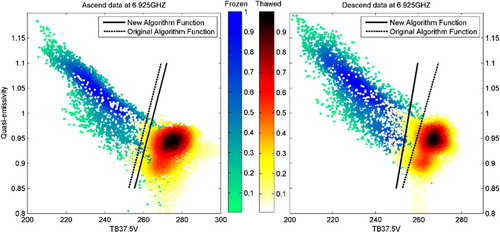
Figure 3. Results of the data separated by Equations (6) and (7) at 10.65 GHz and the original function (colour online).

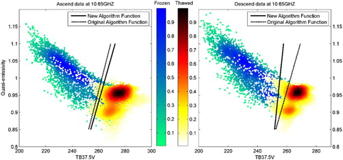
Figure 4. Results of the data separated by Equations (8) and (9) at 18.7 GHz and the original function (colour online).

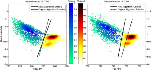
The original discriminant function and the new discriminant function both can disentangle between frozen and thawed soil with the ascend data. But for descend orbit, the original function always seems to overestimate thawed ground, thus making the accuracy of thawed soil low. However, we can see on Figures 2, 3 and 4 that the new discriminant function improves the retrievals, where the thawed points are mostly concentrated in the range of 260–276 K (‘quasi-temperature’) and 0.97–1 (‘quasi-emissivity’), while the frozen points centre in the range of 230–250 K (‘quasi-temperature’) and 1–1.03 (‘quasi-emissivity’), which demonstrate the ability of the two criteria to effectively separate the FT state.

4. Validation and comparison

The classification accuracy of the new DFA is validated against the in-situ soil temperature at 5 cm. The classification accuracy is calculated as the ratio between correct classifications and the total number of instances:(10) $\text{Accuracy}=\frac{\text{FF + TT}}{\text{FF + FT + TF + TT}}\cdot 100\text{\%},$(10) where $\text{FF}$ is a correct frozen classification while $\text{FT}$ is an incorrect case as it is classified as thawed. Similarly, $\text{TT}$ represents a correct thawed classification while $\text{TF}$ is an incorrect case as it is classified as frozen soil.

4.1. Validation with in-situ measurements

In this section, we compare the new DFA with the original one for different orbits using the database composed by all the in-situ soil temperature above. The original function (Zhao et al. 2011) only consider one frequency (18.7 GHz) when calculating the ‘quasi-emissivity’. However, the new function can use three frequencies, represented by the black solid line at 6.925, 10.65 and 18.7 GHz in Figures 2, 3 and 4. Table 2 lists the accuracy of the new discriminant function using 6.9, 10.65 and 18.7 GHz respectively. ‘Frozen (%)’ is the discriminant accuracy of frozen ground, ‘Thawed (%)’ is the discriminant accuracy of thawed soil, and ‘Ascend’ and ‘Descend’ refer to the different orbits of the AMSR-E instrument. The mean discriminant accuracy of ascend orbit, descend orbit, frozen ground and thawed ground were also calculated. The mean accuracy of all the stations at each frequency were all around 90%. Similarly, the mean accuracy of ascend data were around 89% and the mean accuracy of descend data were around 91%. Comparing the accuracy of disparate orbit reveals if the frozen and thawed discriminant accuracy on descend orbit is more balanced. In fact, all the accuracies were around 91%. However, the frozen accuracy of the data was only approximately 84% on ascend orbit while the thawed accuracy could reach as high as 92%. In order to make a contrast with the old discriminant function, Table 3 lists the accuracy of the old function at 18.7 GHz. On the ascend orbit, we can see that the new discriminant function improves the discriminant accuracy of frozen ground for most of cases. On the descend orbit, the original function yields discriminant accuracy of thawed soil as low as 73.3%, while the frozen accuracy is 98.3%. These results reveal the difference between ascend orbit and descend orbit and the need to use two discriminant functions to separate the FT state of the data based on different orbits. The descend data greatly improved through the use of the new function compared with the old algorithm.

Table 2. Accuracy of the new discriminant algorithm function.

Frequency	Orbit	Frozen (%)	Thawed (%)	Mean (%)
6.9 GHz	Ascend	84.30	91.62	88.70
	Descend	84.14	92.02	88.87
	Mean (%)	83.98	92.49	89.09
10.65 GHz	Ascend	90.82	91.38	91.15
	Descend	91.18	90.56	90.81
	Mean (%)	88.91	92.47	91.02
18.7 GHz	Ascend	87.58	91.50	89.92
	Descend	86.46	92.48	90.06
	Mean (%)	86.46	92.48	90.06

Table 3. Accuracy of the original function.

18.7 GHz (original function)
	Frozen (%)	Thawed (%)	Mean (%)
Ascend	82.83	92.93	88.90
Descend	98.32	73.26	83.44
Mean (%)	90.63	83.16	86.17

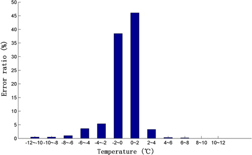
As demonstrated, the new discriminant function clearly improves the discriminant accuracy over the old function; however, it is still not perfect. We analysed the proportion of errors among the different section of temperature of the new algorithm (18.7 and 36.5 GHz) for different orbits (Figures 5 and 6). We found that erroneous classifications generally occurred when soil temperature was close to 0°C for both orbits. Specifically, about 87% of errors on the ascend orbit and about 93% of errors on the descend orbit occurred between −4°C and 4°C. This is likely due to the fact that changes in the FT state of the soil will be more likely and thus more frequent when the soil temperature is near 0°C. With higher frequency changes of state, there is equally a higher chance potential that the instantaneous observation of the satellite will miss the state transformation. Another consideration is that when the soil temperature is near 0°C, the soil is likely to contain both ice and liquid water (L. Zhang et al. 2003). A mixed soil which is transforming between frozen and thawed states will fall in the intersecting region of the new function’s discriminant criteria, thus leading to classification errors. An explanation for why the function may classify soil as frozen when the temperature is above 0°C is that the ground is covered by snow. Conversely, errors in discrimination when the soil temperature is below 0°C could be caused by the melting of snow during the transition from winter to spring. Errors in classification are almost non-existent when the soil temperature is above 4°C but are still present when the soil temperature is below −4°C on both Figures 5 and 6. In other words, among errors in identification, misclassifying frozen soil as the thawed soil is more common in the new discriminant function. This is at least in part due to difference in the depth of the in-situ measured temperatures (i.e. 5 cm), which is deeper than the penetration depth of 18.7 and 36.5 GHz radiation (Ulaby, Moore, and Fung 1982). Here, when the top layer soil (0–2 cm) had thawed, the phase transition of deeper soil had not yet occurred.

Figure 5. Distribution of classification errors among different temperature ranges for the new algorithm (ascending).

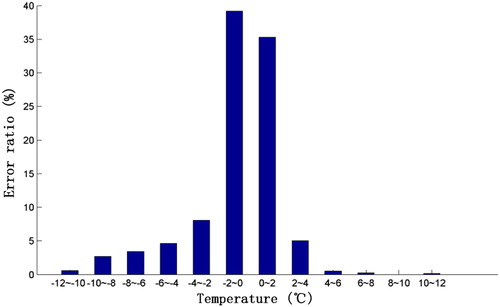
Figure 6. Distribution of classification errors among different temperature ranges for the new algorithm (descending).

4.2. Comparison with the SMAP FTP

In this section, the FT results of the new discriminant algorithm function were compared to the SMAP FT product (SMAP FTP). Since the SMAP FTP is not available until March 2015 while the AMSR-E data covers 2002–2011, in order to evaluate the new function against SMAP FTP, we used the new discriminant function with AMSR2 data. Thus, the AMSR-E inversion algorithm was applied to AMSR2 in order to obtain the long sequence data sets of the land parameters. First of all, we transform the value of AMSR2 brightness temperature into the value of AMSR-E brightness temperature. For 18.7 and 36.5 GHz observations, when using corresponding transformed equations (Hu, Zhao, Shi, and Gu 2016) to compare the two sensors, the correlation reaches 97%, while the root mean square is about 3–6 K and the mean bias is about 0–3 K by comparing the two sensors. The transformed formulas are as follows:(11) $\text{T}{\text{B}}_{\mathrm{A}\mathrm{E}\mathrm{\_}18.7\mathrm{h}}=1.0189\ast T{\text{B}}_{\mathrm{A}2\mathrm{\_}18.7\mathrm{h}}-5.2717,$(11) (12) $\text{T}{\text{B}}_{\mathrm{A}\mathrm{E}\mathrm{\_}18.7\mathrm{v}}=1.0577\ast T{\text{B}}_{\mathrm{A}2\mathrm{\_}18.7\mathrm{v}}-16.204,$(12) (13) $\mathrm{T}{\text{B}}_{\mathrm{A}\mathrm{E}\mathrm{\_}36.5\mathrm{h}}=1.0073\ast T{\text{B}}_{\mathrm{A}2\mathrm{\_}36.5\mathrm{h}}-4.7723,$(13) (14) $\text{T}{\text{B}}_{\mathrm{A}\mathrm{E}\mathrm{\_}36.5\mathrm{v}}=1.0135\ast T{\text{B}}_{\mathrm{A}2\mathrm{\_}36.5\mathrm{v}}-\mathrm{6.3914.}$(14)

We then use the new discriminant algorithm function to calculate the state of the ground in a grid with the transformed brightness temperature and acquire the results of the FT state. Finally, we made a comparison with the SMAP FTP in the same geographic locations. The SMAP FTP of the whole 2016 year was used to compare to the discriminant results of the new discriminant algorithm function. The SMAP sensor overpass times are 06:00 pm (ascending) and 06:00 am (descending), while the corresponding time of AMSR-E and AMSR2 are 01:30 pm and 01:30 am. Hence, it should be note that it exists about five hours’ interval. However, we can compare the results of new discriminant function with the SMAP FTP indirectly. Figure 7 shows the results of a comparison between these two data sets for 2016 at a SMAP FTP core validation site named Cambridge-Bay at 69.15°N, 105.11°W. (Derksen et al. 2017). The ‘New Algorithm Index’ (left Y axis) represents the calculated value by Equations (8) and (9) while the ‘SMAP FTP’ (right Y axis) corresponds to the FT state of SMAP FTP. The blue squares mean the pixel is frozen and the red squares mean the pixel is thawed according to the SMAP FTP. The blue circles and the red circles represent the FT condition calculated by the new algorithm function. The pixel is frozen when the New Algorithm Index value is larger than 0°C and it is thawed when it is less than 0°C. Clearly, there exists a high concordance between SMAP FTP and the discriminant results acquired by the new discriminant function. The accuracy of identification reached about 84.9% for the ascending orbits and 90.4% for the descending orbits when using SMAP FTP as validation. Regardless of the orbit, the ‘New Algorithm Index’ results transition gradually except from March to mid-April, when values fluctuate considerably. This is expected since this time represents a change in seasons where temperature is liable to fluctuate. Figure 7 also shows that there is a delay in the starting date of the freezing or thawing periods between the SMAP FTP and the DFA results. This is primarily due to the five hour offset in overpass time between the two sensors. A comparison of the discriminant results for other SMAP core sites are given in Table 4. The mean accuracy of these sites was about 81.25% (ascending orbit) and 81.11% (descending orbit).

Figure 7. Comparison between SMAP FTP and the results of the new discriminant function at Cambridge-Bay (colour online).

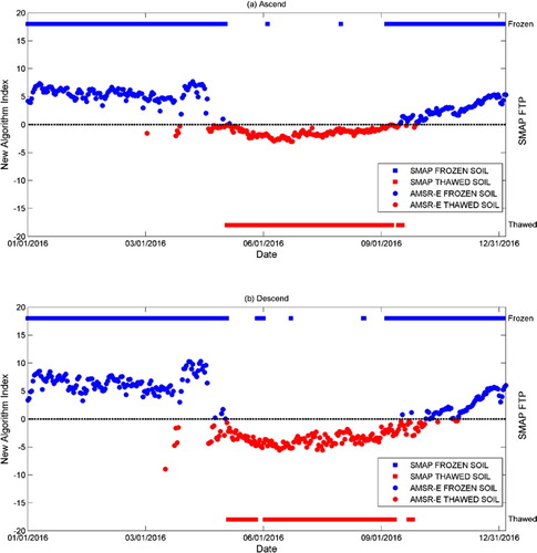
Table 4. Comparison between discriminant results of the new function and SMAP FTP at SMAP core validations sites.

			Comparison analysis
Core site	Country	Location	Ascending orbit (%)	Descending orbit (%)
BERMS-OAS	Canada	53.63 N; 106.20 W	86.81	84.89
BERMS-OBS	Canada	53.99 N; 105.12 W	83.79	84.34
Kenaston	Canada	51.41 N; 106.50 W	79.67	75.82
Sodankyla	Finland	67.36 N; 26.64 E	77.75	75.55
Saariselka	Finland	68.38 N; 27.42 E	83.24	75.82
Imnavait	USA	68.62 N; 149.30 W	70.33	82.69
Baie-James	Canada	53.41 N; 75.013 W	83.52	79.40
Cambridge-Bay	Canada	69.15 N; 105.11 W	84.89	90.38
Mean			81.25	81.11

5. Summary and conclusions

Seasonal frozen soil is widely distributed in the world and is an indicator of climate change. Passive microwave remoting sensing takes the advantages of high temporal resolution and wide spatial coverage, thus playing an important role in the study of the surface FT monitoring. In this article, we use the in-situ soil temperature at 5 cm to parameterize the FT DFA. In addition, the effect of different orbit was considered and two discriminant functions were developed for ascend and descend orbit separately. The precision of the new discriminant function can reach 90% when compared to the in-situ soil temperature at 5 cm. We also compared the FT results determined by the new discriminant function with the SMAP FTP for 2016 and the results show that the new FT discriminant results are generally consistent with the SMAP FTP.

This new discriminant function is, however, not without its limits. First, the algorithm does not consider the effect of earth-covering materials, such as snow and sand. Second, we do not take into account any pixels which contain a water body or lake ice. With these limitations in mind for future research, we aim to use a water distribution maps to avoid the effect of water body or lake ice, and corresponding vegetation models to eliminate the effects of vegetation. We will also conduct further FT experiments of snow-covered ground to determine the radiation characteristics for building simple models to improve the algorithm in the presence of snow.

Acknowledgements

AMSRE, AMSR2 brightness temperature was provided by the GCOM-W Data Providing service, JAXA. The SMAP FTP data can be accessed at the National Snow and Ice Data Center. Pingkai Wang, Tianjie Zhao and Jiancheng Shi contributed to intellectual design and initial drafting. Pingkai Wang compiled and processed data. Pingkai Wang and Tianjie Zhao contributed to data analysis and interpretation. All the authors contributed to the writing of the final draft.

Disclosure statement

No potential conflict of interest was reported by the authors.

ORCID

Hui Lu http://orcid.org/0000-0003-1640-239X

Additional information

Funding

This study was jointly supported by the National Key Basic Research Program of China (2015CB953701), National Natural Science Foundation of China (41671355), Chinese Academy of Sciences Key Research Program of Frontier Sciences (QYZDY-SSW-DQC011), Strategic Pionner Program on Space Science (XDA15052300), ‘Light of West China’ Program and Youth Innovation Promotion Association (No. 2016061). Alexandre Roy was financed by the Canadian Space Agency and the Natural Science and Engineering Research Council of Canada.

References

- Black, T. A., W. J. Chen, A. G. Barr, M. A. Arain, Z. Chen, Z. Nesic, E. H. Hogg, H. H. Neumann, and P. C. Yang. 2000. “Increased Carbon Sequestration by a Boreal Deciduous Forest in Years with a Warm Spring.” Geophysical Research Letters 27 (9): 1271–1274. doi: 10.1029/1999GL011234
- Canny, J. 1986. “A Computational Approach to Edge Detection.” IEEE Transactions on Pattern Analysis and Machine Intelligence PAMI-8 (6): 679–698. doi: 10.1109/TPAMI.1986.4767851
- Derksen, C., X. Xu, R. Scott Dunbar, A. Colliander, Y. Kim, J. S. Kimball, T. Andrew Black, et al. 2017. “Retrieving Landscape Freeze/Thaw State from Soil Moisture Active Passive (SMAP) Radar and Radiometer Measurements.” Remote Sensing of Environment 194: 48–62. doi:10.1016/j.rse.2017.03.007.
- Dobinski, W. 2011. “Permafrost.” Earth-Science Reviews 108 (3–4): 158–169. doi:10.1016/j.earscirev.2011.06.007.
- Du, Toit J. 2007. “The Fourth Assessment Report of the Intergovernmental Panel on Climate Change (IPCC).” Political Science & Politics 36 (3): 423–426.
- Entekhabi, D., E. G. Njoku, P. Houser, M. Spencer, T. Doiron, K. Yunjin, J. Smith, et al. 2004. “The Hydrosphere State (Hydros) Satellite Mission: an Earth System Pathfinder for Global Mapping of Soil Moisture and Land Freeze/Thaw.” IEEE Transactions on Geoscience and Remote Sensing 42 (10): 2184–2195. doi:10.1109/TGRS.2004.834631.
- Entekhabi, D., E. G. Njoku, P. E. O’Neill, K. H. Kellogg, W. T. Crow, W. N. Edelstein, J. K. Entin, et al. 2010. “The Soil Moisture Active Passive (SMAP) Mission.” Proceedings of the IEEE 98 (5): 704–716. doi:10.1109/JPROC.2010.2043918.
- Fisher, R. A. 1936. “The Use of Multiple Measurements in Taxonomic Problems.” Ann Eugenics 7 (2): 179–188. doi: 10.1111/j.1469-1809.1936.tb02137.x
- Frolking, S., K. C. McDonald, J. S. Kimball, J. B. Way, R. Zimmermann, and S. W. Running. 1999. “Using the Space-Borne NASA Scatterometer (NSCAT) to Determine the Frozen and Thawed Seasons.” Journal of Geophysical Research: Atmospheres 104 (D22): 27895–27907. doi: 10.1029/1998JD200093
- Gamon, J. A., K. F. Huemmrich, D. R. Peddle, J. Chen, D. Fuentes, F. G. Hall, J. S. Kimball, et al. 2004. “Remote Sensing in BOREAS: Lessons Learned.” Remote Sensing of Environment 89 (2): 139–162. doi: 10.1016/j.rse.2003.08.017
- Goodison, B. E., R. D. Brown, and R. G. Grane. 1998. “Chapter 6. Cryospheric System.” In EOS Science Plan—The State of Science in the EOS Program, edited by M. D. King, 261–307. NASA Goddard Space Flight Center.
- Han, L., A. Tsunekawa, M. Tsubo, C. He, and M. Shen. 2014. “Spatial Variations in Snow Cover and Seasonally Frozen Ground over Northern China and Mongolia, 1988–2010.” Global and Planetary Change 116: 139–148. doi:10.1016/j.gloplacha.2014.02.008.
- Han, M., K. Yang, J. Qin, R. Jin, Y. Ma, J. Wen, Y. Chen, L. Zhao, Lazhu, and W. Tang. 2015. “An Algorithm Based on the Standard Deviation of Passive Microwave Brightness Temperatures for Monitoring Soil Surface Freeze/Thaw State on the Tibetan Plateau.” IEEE Transactions on Geoscience and Remote Sensing 53 (5): 2775–2783. doi:10.1109/TGRS.2014.2364823.
- Hu Tongxi, Zhao Tianjie, Shi Jiancheng, and Gu Jinzhi. 2016. “Inter-calibration of AMSR-E and AMSR2 Brightness Temperature.” Remote Sensing Technology and Application 31 (5): 919–924. doi: 10.11873/j.issn.1004-0323.2016.5.0919.
- Hu, T., T. Zhao, J. Shi, T. Wang, D. Ji, A. A. Bitar, B. Peng, and Y. Cui. 2016. “Development and Analysis of a Continuous Record of Global Near-Surface Soil Freeze/Thaw Patterns From AMSR-E and AMSR2 Data.” The Cryosphere Discussions: 1–24. doi:10.5194/tc-2016-115.
- Jin, R., X. Li, and T. Che. 2009. “A Decision Tree Algorithm for Surface Soil Freeze/Thaw Classification Over China Using SSM/I Brightness Temperature.” Remote Sensing of Environment 113 (12): 2651–2660. doi:10.1016/j.rse.2009.08.003.
- Jin, R., T. Zhang, X. Li, X. Yang, and Y. Ran. 2015. “Mapping Surface Soil Freeze-Thaw Cycles in China Based on SMMR and SSM/I Brightness Temperatures From 1978 to 2008.” Arctic, Antarctic, and Alpine Research 47 (2): 213–229. doi:10.1657/AAAR00C-13-304.
- Kerr, Y. H., P. Waldteufel, P. Richaume, J. P. Wigneron, P. Ferrazzoli, A. Mahmoodi, A. A. Bitar, et al. 2012. “The SMOS Soil Moisture Retrieval Algorithm.” IEEE Transactions on Geoscience and Remote Sensing 50 (5): 1384–1403. doi: 10.1109/TGRS.2012.2184548
- Kim, Y., J. S. Kimball, K. C. McDonald, and J. Glassy. 2011. “Developing a Global Data Record of Daily Landscape Freeze/Thaw Status Using Satellite Passive Microwave Remote Sensing.” IEEE Transactions on Geoscience and Remote Sensing 49 (3): 949–960. doi:10.1109/TGRS.2010.2070515.
- Kimball, J. S., K. C. Mcdonald, A. R. Keyser, S. Frolking, and S. W. Running. 2001. “Application of the NASA Scatterometer (NSCAT) for Determining the Daily Frozen and Nonfrozen Landscape of Alaska.” Remote Sensing of Environment 75 (1): 113–126. doi: 10.1016/S0034-4257(00)00160-7
- Kimball, J. S., K. C. McDonald, S. W. Running, and S. E. Frolking. 2004. “Satellite Radar Remote Sensing of Seasonal Growing Seasons for Boreal and Subalpine Evergreen Forests.” Remote Sensing of Environment 90 (2): 243–258. doi:10.1016/j.rse.2004.01.002.
- Kimball, John S., and Kyle C. Mcdonald. 2004. “Satellite Observations of Annual Variability in Terrestrial Carbon Cycles and Seasonal Growing Seasons at High Northern Latitudes.” Proceedings of SPIE - The International Society for Optical Engineering 5654.
- Lobl, Elena, Roy W. Spencer, Keiji Imaoka, and Keizo Nakagawa. 2010. “AMSR-E and its follow-on, AMSR2.” Geoscience and Remote Sensing Symposium, 2009 IEEE International, igarss, Vol. 3, pp. III-77-III-80. IEEE.
- Mcfarland, M. J., R. L. Miller, and C. M. U. Neale. 1990. “Land Surface Temperature Derived From the SSM/I Passive Microwave Brightness Temperatures.” IEEE Transactions on Geoscience and Remote Sensing 28 (5): 839–845. doi: 10.1109/36.58971
- Oechel, W. C., G. L. Vourlitis, S. J. Hastings, R. C. Zulueta, L. Hinzman, and D. Kane. 2000. “Acclimation of Ecosystem CO2 Exchange in the Alaskan Arctic in Response to Decadal Climate Warming.” Nature 406 (6799): 978–981. http://www.nature.com/nature/journal/v406/n6799/suppinfo/406978a0_S1.html. doi: 10.1038/35023137
- Oliva, R., E. Daganzo, Y. H. Kerr, S. Mecklenburg, S. Nieto, P. Richaume, and C. Gruhier. 2012. “SMOS Radio Frequency Interference Scenario: Status and Actions Taken to Improve the RFI Environment in the 1400–1427-MHz Passive Band.” IEEE Transactions on Geoscience and Remote Sensing 50 (5): 1427–1439. doi: 10.1109/TGRS.2012.2182775
- Panneer Selvam, B., H. Laudon, F. Guillemette, and M. Berggren. 2016. “Influence of Soil Frost on the Character and Degradability of Dissolved Organic Carbon in Boreal Forest Soils.” doi:10.1002/2015JG003228.
- Rautiainen, K., J. Lemmetyinen, J. Pulliainen, J. Vehvilainen, M. Drusch, A. Kontu, J. Kainulainen, and J. Seppanen. 2012. “L-Band Radiometer Observations of Soil Processes in Boreal and Subarctic Environments.” IEEE Transactions on Geoscience and Remote Sensing 50 (5): 1483–1497. doi:10.1109/TGRS.2011.2167755.
- Rawlins, M. A., K. C. McDonald, S. Frolking, R. B. Lammers, M. Fahnestock, J. S. Kimball, and C. J. Vörösmarty. 2005. “Remote Sensing of Snow Thaw at the pan-Arctic Scale Using the SeaWinds Scatterometer.” Journal of Hydrology 312 (1): 294–311. doi: 10.1016/j.jhydrol.2004.12.018
- Rignot, E., and J. B. Way. 1994. “Monitoring Freeze—Thaw Cycles Along North—South Alaskan Transects Using ERS-1 SAR.” Remote Sensing of Environment 49 (2): 131–137. doi: 10.1016/0034-4257(94)90049-3
- Roy, A., A. Royer, J. P. Wigneron, A. Langlois, J. Bergeron, and P. Cliche. 2012. “A Simple Parameterization for a Boreal Forest Radiative Transfer Model at Microwave Frequencies.” Remote Sensing of Environment 124 (2): 371–383. doi: 10.1016/j.rse.2012.05.020
- Roy, A., P. Toose, C. Derksen, T. Rowlandson, A. Berg, J. Lemmetyinen, A. Royer, E. Tetlock, W. Helgason, and O. Sonnentag. 2017. “Spatial Variability of L-Band Brightness Temperature During Freeze/Thaw Events Over a Prairie Environment.” Remote Sensing 9 (12): 894. doi:10.3390/rs9090894.
- Schuur, E. A. G., J. Bockheim, J. G. Canadell, E. Euskirchen, C. B. Field, S. V. Goryachkin, S. Hagemann, et al. 2008. “Vulnerability of Permafrost Carbon to Climate Change: Implications for the Global Carbon Cycle.” BioScience 58 (8): 701–714. doi:10.1641/B580807.
- Ulaby, Fawwaz T., Richard K. Moore, and Adrian K. Fung. 1982. Microwave Remote Sensing Active and Passive-Volume II: Radar Remote Sensing and Surface Scattering and Enission Theory. Reading, MA: Addison-Wesley, Advanced Book Program.
- Way, J. B., R. Zimmermann, E. Rignot, K. McDonald, and R. Oren. 1997. “Winter and Spring Thaw as Observed with Imaging Radar at BOREAS.” Journal of Geophysical Research: Atmospheres 102 (D24): 29673–29684. doi:10.1029/96JD03878.
- Xu, X., R. S. Dunbar, C. Derksen, A. Colliander, Y. Kim, and J. S. Kimball. 2016. SMAP L3 Radiometer Northern Hemisphere Daily 36 km EASE-Grid Freeze/Thaw State, Version 1. [Indicate subset used]. Boulder, CO: NASA National Snow and Ice Data Center Distributed Active Archive Center. https://doi.org/10.5067/RDEJQEETCNWV.
- Zhang, T., and R. L. Armstrong. 2001. “Soil Freeze/Thaw Cycles over Snow-Free Land Detected by Passive Microwave Remote Sensing.” Geophysical Research Letters 28 (5): 763–766. doi: 10.1029/2000GL011952
- Zhang, T., R. L. Armstrong, and J. Smith. 2003. “Investigation of the Near-Surface Soil Freeze-Thaw Cycle in the Contiguous United States: Algorithm Development and Validation.” Journal of Geophysical Research: Atmospheres 108 (D22): S80–S85.
- Zhang, T., R. G. Barry, K. Knowles, J. A. Heginbottom, and J. Brown. 1999. “Statistics and Characteristics of Permafrost and Ground-ice Distribution in the Northern Hemisphere.” Polar Geography 23 (2): 132–154. doi:10.1080/10889379909377670.
- Zhang, T., J. A. Heginbottom, R. G. Barry, and J. Brown. 2000. “Further Statistics on the Distribution of Permafrost and Ground ice in the Northern Hemisphere.” Polar Geography 24 (2): 126–131. doi:10.1080/10889370009377692.
- Zhang, L., J. Shi, Z. Zhang, and K. Zhao. 2003. “The Estimation of Dielectric Constant of Frozen Soil-Water Mixture at Microwave Bands.” Geoscience and Remote Sensing Symposium, 2003. IGARSS ‘03. Proceedings. 2003 IEEE International.
- Zhao, T., L. Zhang, L. Jiang, S. Zhao, L. Chai, and R. Jin. 2011. “A new Soil Freeze/Thaw Discriminant Algorithm Using AMSR-E Passive Microwave Imagery.” Hydrological Processes 25 (11): 1704–1716. doi:10.1002/hyp.7930.
- Zuerndorfer, B., and A. W. England. 1992. “Radiobrightness Decision Criteria for Freeze/Thaw Boundaries.” IEEE Transactions on Geoscience & Remote Sensing 30 (1): 89–102. doi: 10.1109/36.124219