Quantifying local fire regimes using the Landsat data-archive: a conceptual framework to derive detailed fire pattern metrics from pixel-level information

ABSTRACT

Free and open access to the Landsat archive has enabled the detection and delineation of an unprecedented number of fire events across the globe. Despite the availability and potential of these data, few studies have analysed residual vegetation patterns and/or partial mortality of fire across the Canadian boreal forest, and those available, are either incomplete or inaccurate. Further, they all differ in the methods and spatial language, which makes it difficult for managers to interpret fire patterns over large areas. There is an urgent need for methods to help unify fire pattern observations across the Canadian boreal forest. This study explores the capacity of the Landsat data archive when coupled with a recently developed fire mapping approach and a robust spatial language to characterize and compare tree mortality patterns across the boreal plains ecozone, Canada. With 507 fires 2.5 Mha mapped, this study represents the most comprehensive analysis of mortality patterns for study area. Summaries from this demonstration generated an accurate characterization of the fire patterns the various ecoregions based on seven key fire metrics. The comparison between ecoregions revealed differences in the amount of residual vegetation, which in turn suggested various climate, topography and/or vegetation ecosystem drivers.

KEYWORDS:

• Fire emulation
• historical range of variability
• landscape metrics
• fire patterns
• disturbance-based management

1. Introduction

In the last decade multiple forest management agencies across Canada have adopted a disturbance-based approach to harvesting, where historical, natural fire patterns are used as a guide to maintain a range of ecosystem conditions (Hunter 1993; Landres, Morgan, and Swanson 1999). In fact, most provinces and certification agencies in Canada now require forest management plans to include some level of natural pattern approximation (Perera 2014), including guidelines for stand structure retention (e.g. OMNR 2001). Relevant to the implementation of such approaches is to define and characterize local fire regimes (Boulanger et al. 2013): how much, where, how often, and why do fires burn what they do? In particular, the characterization of smaller and/or partial mortality remnants whose amount and spatial configuration are important for forest succession (Kane et al. 2015), habitat refugia (Banks et al. 2011), and re-vegetation patterns (Oliver 1980).

Fire patterns vary greatly, both between and within fires, in response to environmental conditions at multiple temporal and spatial scales (Loehman, Reinhardt, and Riley 2014). In fact, there is evidence to suggest that wildfire patterns are regionally unique (Andison and McCleary 2014; Burton et al. 2008; Madoui et al. 2010; Parisien et al. 2006), which means that capturing the complexity of fire patterns across large areas like the Canadian boreal forest requires extensive and detailed fire pattern information. Conventional methods to map fire mortality patterns are via manual delineation of polygons of different tree mortality classes within a fire perimeter from very high-resolution aerial images (Morgan, Gergel, and Coops 2010). Fire mortality data generated by this method are highly accurate and precise, however, are expensive and time-consuming to produce, and are geographically limited to areas of existing aerial photo coverage (Wulder 1998). A Canadian wildfire dataset of 129 wildfires (30–25,000 ha) that burned between 1940 and 2010 across Alberta and Saskatchewan (Andison and McCleary 2014) offers a prime example of these detailed and valuable databases.

Over continental scales and multi-decadal time frames satellite remotely sensed data have great potential to capture changes in vegetation condition (Wulder et al. 2008). The recent opening of the United States Geological Survey (USGS) archive of Landsat imagery (Woodcock et al. 2008) has provided users with high-quality data processed to stringent radiometric and geometric standards that is suitable for time-series analysis of vegetation condition (Zhu and Woodcock 2014). The increased data availability has enabled the development of multiple algorithms to detect and mask noise and data fusion techniques to guarantee spectral consistency across the time series (White et al. 2014). For example, the Fmask algorithm developed by Zhu and Woodcock (2012) is now routinely applied to the entire Landsat data archive providing a user-ready mask with information about water, clouds, shadows and other atmospheric distortions (https://espa.cr.usgs.gov/). Similarly, the development of pixel-compositing approaches to combine and summarize dense and noisy time-series imagery into seamless spectrally consistent, cloud-free images can be used to detect and quantify changes in vegetation condition (White et al. 2014). Together these advancements make possible the detection and delineation of fires across unprecedented spatial scales (Hermosilla et al. 2016; White et al. 2017), the detailed characterization of changes in vegetation condition (Eidenshink et al. 2007) and the study of recovery trends after disturbance (Kennedy, Yang, and Cohen 2010).

Despite the availability and potential of these data, there have been no studies that have captured detailed residual patterns and partial mortality with reasonable accuracy on anything more than a very small sample size across the Canadian boreal forest. One of the major reasons this is so challenging is that Landsat requires an independent source of data for calibration and validation. Without this, it is not possible to evaluate the accuracy of the mortality maps, rendering the results un-defendable for managers (e.g. Burton et al. 2008). Composite Burn Index (CBI) field data (Key and Benson 2006) has become the standard for burn severity mapping as a quick method to assess ground measurements of fire effects for map calibration and accuracy assessment of burn severity maps (Eidenshink et al. 2007). CBI plots record rankings from 0 (unburned) to 3 (most severe) across different strata (soil, understory, shrub, intermediate trees and overstory trees), which are then averaged to a unitless value (Key and Benson 2006). Few studies across the Canadian boreal forest have used Landsat and CBI data with moderate to highly significant relationships (overall R² from 0.66 to 0.84) (Boucher et al. 2017; Hall et al. 2008; Soverel, Perrakis, and Coops 2010). However, there are some challenges to using CBI data. First, collecting CBI data over remote areas is highly expensive and would require a vast network of plots to capture the variability of conditions in highly heterogeneous boreal landscapes (Fraser, van der Sluijs, and Hall 2017). The result is a series of scattered studies with low sample sizes (<10) (Boucher et al. 2017; Hall et al. 2008; Soverel, Perrakis, and Coops 2010) that offer little context to interpret the variability of fire patterns within and among fires across even moderately-sized areas. Other challenges to utilizing CBI for fire pattern studies include that its visual assessment is somewhat subjective and highly variable among observers (Lentile et al. 2006) and lacking a clear agreed-upon biometric definition (Kolden, Matthew, and Smith 2016), which hinders the comparability and interpretability of the results. Given the applied nature of the fire mortality pattern information to forest management, regulatory, and certification agencies, incomplete or inaccurate fire pattern estimates are not defendable, and thus of limited value. Another significant challenge associated with the existing fire mortality studies in the Canadian boreal is the inability to compare results between studies. All of the available studies differ in their methods, data quality and type, and spatial language, which makes difficult for managers to understand and compare fire patterns across large areas. For example, Andison (2012) demonstrated that even subtle changes to the definition of a fire event can have dramatic impacts on the amount of residual vegetation.

Thus there is an increasing need to characterize detailed tree mortality patterns of wildfire in a systematic, accurate and comprehensive way across the boreal forest. This information can then be used to quantify how fire pattern metrics vary among and within pre-defined ecological zonations (e.g. Parisien et al. 2004), to define areas were fire regimes are relatively homogeneous (Boulanger et al. 2012), or to better understand the relationship between fire pattern metrics and various environmental variables (Morgan et al. 2001). If broad-scale patterns are found to exist, they would increase the robustness of statistic inferences across the broader expanse of the Canadian boreal forest in support to management efforts.

Recently, San-Miguel, Andison, and Coops (2017) developed a Landsat-based model to cost-effectively generate seven fire event characteristics based on a three-class mortality map (unburned, partial mortality and complete mortality) coupled with the spatial language proposed by Andison (2012). The method utilizes a random forest (RF) classifier (Breiman 2001) combining as training data aerial photo-interpreted (API) polygons of mortality and as predictor variables multiple multi-temporal Landsat spectral variables (such as the differenced Normalized Burn Ratio (dNBR) by Key and Benson [2006]) and complementary geospatial variables (such as land cover and topography). The model was calibrated to the area of study by using detailed mortality polygons covering 14 fires across the boreal plains (BP) ecozone, Canada. Once calibrated, this model was used to produce mortality maps for other fires using predictor variables derived from Landsat and ancillary data.

We believe there are several advantages to using polygons of tree mortality to map fire patterns. First, in forested systems, Landsat burn severity products are highly correlated to fire effects on overstory vegetation (Lentile et al. 2006; Miller and Thode 2007; Fraser, van der Sluijs, and Hall 2017) and less so with the obscured sub-canopy effects that are also captured in CBI (Cocke, Fulé, and Crouse 2005). Second, API can provide a cheaper and quicker alternative to producing validation data for burn severity studies, which will help in cost-effectively covering much larger areas. Third, polygons of tree mortality are spatially continuous rather than plot-based, which better capture the variability of fire effects across the fire event. Lastly, canopy mortality is estimated via a direct measurement of a single variable, rather than a composite index aggregating multiple strata. This provides a more concrete basis to map fire patterns with satellite-derived data that can augment the comparability of results across ecological conditions and be more useful for managers.

The San San-Miguel, Andison, and Coops (2017) fire pattern model requires (1) a buffered perimeter to identify the Landsat scenes covering the area of study and, (2) the year of fire occurrence to determine the dates of the pre- and post-fire images needed for the analysis. Overall the Landsat method produced comparable results to those observed from API, both at the regional scale of all fires combined and at the scale of single fire events. The technique captured the outer perimeter and the total amount of vegetation residuals with high accuracy, although misclassified a small portion (6%) of the partially burned areas as unburned (San-Miguel, Andison, and Coops 2017). There are several reasons for the difficulty in capturing partial mortality which have been reported in other studies. For example, partially disturbed areas are generally patchier and of smaller size than their completely burned counterparts, making them more difficult to capture with the 30-m pixel size of Landsat Thematic Mapper (TM) due to mixed fire effects (Lentile et al. 2006). Also, plant regrowth following fire and delayed mortality sometimes masks the changes in reflectance in burned areas (Key and Benson 2006). Despite these challenges, the San-Miguel, Andison, and Coops (2017) study provides a strong model that predicts key fire pattern metrics with accuracy levels close to that of those from API. The opportunity to couple this model with the ability to use freely and widely available Landsat makes this technique well suited for capturing and comparing detailed mortality patterns of hundreds of wildfires across vast areas, and thus potentially a valuable new tools for both researchers and forest managers. However, the degree to which this approach can be successfully applied across large areas remains untested.

In this paper, we explore the capacity of a recently developed standardized fire mapping approach by San-Miguel, Andison, and Coops (2017) using Landsat data and the spatial language by Andison (2012), to characterize, summarize and compare fire mortality patterns in the BP ecozone of Canada. It is important to note that the detection model applied to these fires was an entirely separate analytical step that was part of another study (San-Miguel, Andison, and Coops 2017). Our hypothesis is that Landsat-based approach can be used to capture and compare fire patterns to a sufficient degree of accuracy and completion across the boreal biome to support management efforts. The results will not only allow the collection of quantitative fire pattern information on an unprecedented scale, but also new insights into the most appropriate scales to characterize local fire regimes to support disturbance-based management approaches and a broad range of associated research studies. We also discuss the big data processing decisions and related outcomes for large area mapping of hundreds of fires over the region.

2. Study area

The BP is the third largest ecozone in Canada (Canadian Forest Service 2013), covering the provinces Manitoba, Saskatchewan and Alberta and extensions of northeastern British Columbia and south-central Northwest Territories (Figure 1). The climate is humid continental with cold winters and moderately warm summers. The precipitation ranges from 300 to 500 mm in average, typically increasing from north to south and west to east. The area consists of low-lying valleys and plains, dominated by dense to sparse coniferous and mixedwood forests, with a mosaic of trees, shrubs, herbs, wetlands and lakes (Ecological Stratification Working Group 1996). The main tree species are black spruce (Picea mariana P. Mill.), white spruce (Picea glauca Moench), jack pine (Pinus banksiana Lamb.) and tamarack (Larix lariciana Du Roi) which are capable of tolerating the long, cold winters characteristic of this ecozone. Broadleaf species, such as trembling aspen (Populus tremuloides Michx.), white birch (Betula papyrifera Marshall) and balsam poplar (Populus balsamifera L.), are more abundant towards the southern portion of the ecozone (Ecological Stratification Working Group 1996). In terms of land cover uses, a 76% of the BP is allocated to forestry, followed by conservation (figures of protection) (15%), with smaller contributions of agriculture, oil and gas exploration and settlements (Canadian Forest Service 2013). The BP region is also important for the forestry economy in Canada as it holds an 11% of the total tree volume (Canadian Forest Service 2013). The BP is divided into 10 ecoregions, or broad recurring vegetation and landform patterns, within the regional climatic context of the ecozone (Table 1).

Figure 1. Fire sample across the boreal plains ecozone.

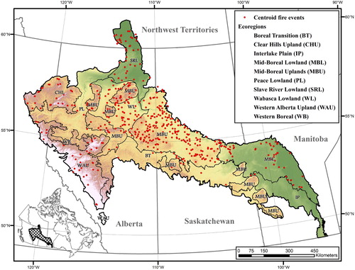
Table 1. Physical and biological characteristics of the ecoregions with 30 or more fires within the BP ecozone. Based on the Terrestrial Ecozones of Canada (Wiken 1986).

Ecoregion name	Ecoclimate	Mean temperatures for year/summer/winter (°C)	Precipitation (mm)	Vegetation	Topography	Remarks	N of fires in the sample
Slave River Lowlands (SRL)	Sub humid mid-boreal	−2/13/−17	300–400	Closed stands of trembling aspen, balsam poplar, and jack pine with white and black spruce, and balsam fir in late successional stages. Tamarack and black spruce dominate fens and bogs with ericaceous shrubs and mosses	Flat to gently rolling	50% of the area is peatlands	38
Clear Hills Upland (CHU)	Sub humid mid-boreal	−1/13/−17	400–600	Lodgepole pine with white spruce and fir in the uplands. Black spruce dominates in the poorly drained valley bottoms	Steep to gently rolling	Ecotone between boreal and cordilleran vegetation	30
Mid-Boreal Uplands (MBU)	Sub humid mid-boreal	−1/14/−14	400–550	Closed stands dominated by trembling aspen with balsam poplar with understory of tall shrubs and herbs. White and black spruce, and balsam fir occur in late successional stages. Deciduous stands have and understory of tall shrubs and herbs while coniferous have feathermoss. Tamarack and black spruce dominate fens and bogs	Flat to gently rolling	Accounts for most area burnt in BP (Parisien et al. 2004)	275
Wabasca Lowland (WL)	Sub humid mid-boreal	1/13/−13	350–500	Closed stands of trembling aspen and balsam poplar. White and black spruce, and balsam fir, occur in late successional stages. Tamarack and black spruce dominate fens and bogs	Flat to gently rolling	50% of the area is peatlands	53
Western Alberta Upland (WAU)	Sub humid mid-boreal	1.5/12/−10	450–600	Closed stands dominated by lodgepole pine, trembling aspen and white spruce with some balsam poplar, paper birch and balsam fir. Drier sites are most often covered by stands of aspen or open lodgepole pine forest; while on wet sites tamarack and black spruce are more prevalent. Higher elevations of the foothills are dominated by conifers and lower plains with aspen	Flat to gently rolling	Ecotone between mid-boreal and mid-cordilleran vegetation	35
Mid-Boreal Lowland (MBL)	Sub humid mid-boreal	−1/13/−17	375–625	Closed stands of trembling aspen, balsam poplar, and jack pine with white and black spruce, and balsam fir in late successional stages. Black spruce and willows dominate fens and bogs	Flat	50% wetlands	51

Wildfire is the most prevalent natural disturbance agent in the area, with smaller contributions from insects, disease, and wind (Brandt 2009; White et al. 2017). Historical fire cycles in the BP are in average around 250 years (Parisien et al. 2004; Stocks et al. 2002), but with substantial inter-annual variability and among ecoregions (Parisien et al. 2004). Anthropogenic disturbances are more common in southern areas of the ecozone, where the accessibility is greater, harvest tenures older and more common and fire suppression more temporally consistent over the last 60 years.

3. Methods

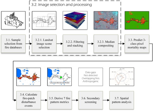
The developed method is summarized in Figure 2 and briefly described below. First, from existing fire history databases (described below) we selected all available fires larger than 100 ha which occurred within the BP from 1985 to 2014 (Section 3.1) and downloaded, pre-processed and merged the Landsat imagery into seamless cloud-free surface-reflectance composites (Section 3.2). Next, for each fire, we produced a three-class mortality map using a RF classifier previously trained with manually interpreted polygons of tree mortality from aerial imagery and multi-temporal spectral indices calculated from the Landsat composites and ancillary data (Section 3.3). Based upon the pixel mortality predictions for each fire, we then calculated discrete patch disturbance events based on the spatial language by Andison (2012) (Section 3.4) and derived seven fire pattern metrics of interest for managers (Section 3.5). Next, we screened out the predictions that were not consistent with the reference perimeters from the fire databases (Section 3.6). Finally, we pooled the results from all fires and analysed the variability of the fire pattern metrics across the full fire sample and the ecoregions within (Section 3.7). A description of each step is given in Figure 2.

Figure 2. Analysis workflow.

3.1. Sample selection from fire databases

As reference data for this study, we captured as many previously identified historical wildfires as possible from the BP ecozone that occurred between 1985 and 2014 that were at least 100 ha in size. We sampled from three publically available sources (i) the federal Canadian Fire and (ii) provincial fire databases, as well as (iii) fire events with perimeters derived from the High Resolution Forest Change (HRFC) for Canada product (White et al. 2017; accessed via https://opendata.nfis.org/mapserver/nfis-change_eng.html). This initial screening process yielded 1147 fires across 5.3 Mha. From each fire, we retained the perimeter and the fire year.

3.2. Image selection and processing

3.2.1. Landsat image scene selection

For each fire that met the above criteria, we used fire year and perimeter (which included a 20 km buffer to allow for mapping errors) to select the corresponding pre- and post-fire Landsat images. The pre-fire temporal window was between one and six years prior to the fire. Lengthening the pre-fire temporal window minimized the chances of gap occurrence (mostly due to cloud coverage) while still representing a relatively static picture of low productivity boreal ecosystems. The post-fire temporal window included images from one to two years after the fire, which aligns well with the extended assessment (EA) proposed by Key and Benson (2006). EA better portrays the long-term ecological effects of fire accounting for delayed tree mortality and secondary mortality agents (Key and Benson 2006), and has been most often used in burn severity mapping of forested and shrub systems (Eidenshink et al. 2007; French et al. 2008). Candidate Landsat imagery included LT-1 corrected-products from Landsat TM, Enhanced Thematic Mapper Plus (ETM+) and Operational Land Imager (OLI) from the USGS archive over all fires within the defined pre- and post-fire windows. We selected a 130 day window from each fire event (from mid-May to mid-September) to maximize the number of Landsat images while avoiding images before vegetation green-up or after vegetation senescence, reducing probability of snow presence, and minimizing the chances of classification errors associated to low-sun elevation angles late in the fire season (Verbyla, Kasischke, and Hoy 2008). To reduce the processing times, we removed scenes with more than 80% cloud cover estimation from the Fmask layer (Zhu and Woodcock 2012) included in the image metadata. All candidate images were sent to the USGS ESPA platform (http://espa.cr.usgs.gov) to be processed to surface-reflectance products and downloaded.

3.2.2. Filtering and stacking

From all the Landsat ESPA layers we retained the red, near (NIR) and shortwave infrared (SWIR) portions of the spectrum since they are the most responsive to changes in vegetation condition (i.e. 3, 4, 5 and 7 in Landsat TM/ETM+; and 4, 5, 6 and 7 for OLI) (Pereira et al. 1999); and the water mask of water from the Fmask layer. We also utilized the Fmask to mask out pixels flagged as cloud or near cloud (distance < 150 m), as well as cloud shadows and haze (atmospheric opacity < 200).

3.2.3. Median compositing

While most noise was removed from the Landsat imagery by using the procedures described above, undetected clouds, smoke or haze from single date cloud detection (Zhu and Woodcock 2012) can lead to a false detection of change. To select representative pixels for the pre- and post-fire image composites we used a median compositing approach to produce seamless cloud-free composites as it is robust against outliers (White et al. 2014), can be directly applied to the filtered image stacks and, unlike the spectral trend analysis algorithms (as in Hermosilla et al. [2016] or Kennedy, Yang, and Cohen [2010]), can be computed over shorter temporal windows to help reduce data volumes and processing times. We also created a water layer mask with the pixels classified as water by the Fmask in more than 60% of the total valid observations, similar to methods of Hermosilla et al. (2016).

3.3. Predict three-class pixel mortality maps

To produce tree mortality maps for single fires we utilized a RF classifier (Breiman 2001) previously trained with API polygons for 14 fires across the BP ecozone and a suite of explanatory variables to characterize the spectral response of fire effects (San-Miguel, Andison, and Coops 2017). Tree mortality was defined as the percentage of crown mortality of overstory vegetation and/or consumption of lesser vegetation, and was classified into three classes: unburned = 0–5%, partial mortality = 6–94%, and complete mortality ≥ 94. The explanatory variables for the RF classifier included the difference in the green, NIR and SWIR Landsat bands (i.e. 3, 4, 5 and 7 in Landsat TM/ETM+), the dNBR (Key and Benson 2006) that is based on the NBR by García and Caselles (1991) and responsive to changes in live vegetation (NIR), moisture content, mineral soil exposure, char and ash occurrence (SWIR) (Miller and Thode 2007) that is highly correlated to changes in canopy cover (Mccarley et al. 2017); and the differenced Normalized Difference Vegetation Index (dNDVI) (Rouse et al. 1974) to improve the characterization of forest structure and photosynthetic activity (Bolton, Coops, and Wulder 2015). In addition we included an assessment of pre-fire vegetation condition through the pre-fire NBR and NDVI, the land cover class from the Earth Observation for Sustainable Development of Forests (EOSD) product (Wulder et al. 2007); as well as topographic information derived from the Shuttle Radar Topography Mission (SRTM) 1 arc second global product, which included aspect, slope angle and terrain roughness, calculated as the difference in metres between the value of a cell and the mean value of its eight surrounding cells (Wilson et al. 2007).

To provide spatial context for the classification (Morgan and Gergel 2010), we summarized the pixel-level explanatory variables by segments and incorporated them as additional explanatory variables to the RF classifier. To do this the mean-shift algorithm implemented in the Orfeo Toolbox (Christophe, Inglada, and Giros 2008) was used on the dNBR values (Key and Benson 2006). The approach requires two inputs: a spatial radius and a range value. The spatial radius is the distance in pixels to be utilized for the search window. The range value is the maximum radiometric distance in the multispectral space. For each pixel, the mean-shift algorithm calculates a vector with the pixels within the spatial range whose value is within the radiometric range. The method iteratively shifts the centre of window to the pixel suggested by the vector until it finds a local maximum of density. All the initial pixels that converged to the same local maxima are considered to be members of the same cluster. For the segmentation, we utilized a spatial range of 50 pixels and a spatial radius of 5 pixels.

3.4. Calculate fire-patch disturbance events

Pixel-level mortality maps were converted into discrete fire-patch disturbance events using the spatial language of Andison (2012). Three types of patches are defined: disturbed, island remnants and matrix remnants. The disturbed class corresponds to areas that underwent complete mortality. The island remnants comprise the vegetation that survives in some form within the event perimeter and serves as starting point from biotic reassembly (Perera 2014), such as providing refugia for small mammals and seed sources for tree recolonization (Banks et al. 2011; Eberhart and Woodard 1987). The matrix remnants represent undisturbed vegetation residuals that lie beyond the boundaries of disturbed patches, and that serve as corridors or peninsulas between disturbed patches (Andison 2012). The island remnants class comprises a broad range of mortality which makes easier to calculate and interpret broad fire pattern metrics. Multiple studies have already used this nomenclature to inform management plans across the Canadian boreal forest. For example, Pickell, Andison, and Coops (2013) used it to quantify deviances from the natural variability of various harvesting and oil exploration treatments in northern Alberta; and Andison and McCleary (2014) to compare fire patterns across multiple sub-regions across the western Canadian boreal forest.

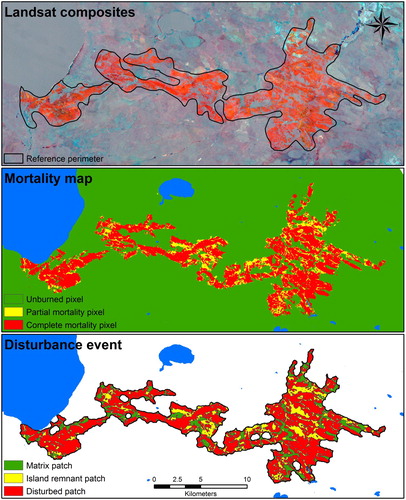
We calculated the disturbance events as follows. First, adjacent similar pixel types were merged into individual polygons based on eight neighbours. Second, we delineated the boundaries of individual disturbed patches within each wildfire by merging all adjacent disturbed and island polygons. Third, we buffered out, and then back in 200 m from the disturbed patches, to define the boundary of the fire event. The new residual areas created by this buffering exercise are matrix remnants (Andison 2012). Lastly, water pixels were masked from the disturbance event. For the purpose of this study, we only retained the disturbance events intersecting with the reference perimeter from the fire databases. Figure 3 shows an example of the complete process, from the image mosaics to defining the disturbance events.

Figure 3. Process to derive a disturbance event.

Notes: The top thumbnail represents the difference between pre- and post-fire composites, where the red channel corresponds to the difference in Landsat NIR band (4 in TM and 5 in OLI), the green channel to the difference in the SWIR 1 band (5 in TM and 6 in OLI) and the blue channel the difference in the SWIR 2 band (7 in TM and OLI). The middle thumbnail represents the three-class mortality map from the RF classifier, where green corresponds to unburned, yellow to partial mortality and red complete mortality. The bottom figure corresponds to the disturbance event by Andison (2012), where red corresponds to disturbed, yellow to IR and dark green to MR (colour online only).

3.5. Derive seven fire pattern metrics

For each disturbance event, we calculated seven fire pattern metrics initially proposed by Andison (2012) to represent key fire pattern characteristics, since tested by San-Miguel, Andison, and Coops (2017). To characterize the size and complexity of the fire event perimeter, we used the event area (EA) and the shape index (SI) metrics, respectively. To characterize the details of the amount and spatial arrangement of the mortality within each event we used the percentage of total remnants (%TR), the percentage of island remnants (%IR), the percentage of matrix remnants (%MR), the number of disturbed patches (NDP) and the percentage of largest disturbed patch (%LDP) (see details in Table 2). The seven metrics were assigned to a point at the centroid of each disturbance event in our sample.

Table 2. Description of the seven fire pattern metrics calculated on the disturbance events. Based on Andison (2012).

Type	Metric [unit]	Acronym	Formula	Interpretation
Event	Event area [ha]	EA	MR + IR + disturbed	Size of the event
	Shape index [no units]	SI	Total perimeter of the disturbance event/perimeter of a square with area of EA	Complexity of the perimeter
Within-event	Percentage of matrix remnants [%]	%MR	(Total area of MR/EA) × 100	Percentage of residuals physically attached to the surrounding matrix of intact forest
	Percentage of island remnants [%]	%IR	(Total area of IR/EA) × 100	Percentage of residuals lying entirely within disturbed patches
	Percentage of total remnants [%]	%TR	((Total area of IR + total area of MR)/EA) × 100	Percentage of vegetation that survives in some form
	Number of disturbed patches [patches]	NDP	Number of patches resulting of the combination of IR and disturbed classes	Total number of disturbed patches per event
	Percentage largest disturbed patch [%]	%LPD	(Area of the LDP/EA) × 100	Size variability of disturbed patches

3.6. Secondary screening

The last data processing step was to filter out fire events that were not consistent with the fire perimeters utilized for reference, to avoid possible biases during the spatial pattern analysis. A secondary screening process consisted of a sequence of automated quality control steps followed by a visual evaluation of the results. First, we removed the fire events for which the mortality maps presented more than 5% of data gaps in the mortality prediction within or near (1 km) the perimeters suggested by the fire databases. Second, we removed the fires events that were not detected (i.e. all unburned pixels from the mortality maps) or covered less than 30% of the area suggested by the reference perimeters. Finally, through visual inspection we discarded the disturbance events that included adjacent contemporaneous fire events or with signs of anthropogenic activity (harvesting cutblocks).

3.7. Spatial pattern analysis

To explore the variability in fire patterns we pooled the results from single events and summarized and compared the seven pattern metrics using a combination of box-and-whisker plots and spyder plots calculated on median values. Spyder plots show the relative values for a single data point given an arbitrary number of variables, and are useful to highlight similarities or differences in the fire pattern metrics among the ecoregions. To guarantee sufficient data representation, we did not consider the ecoregions with less than 30 fires. To test for differences in fire pattern metrics we compared the cumulative distributions functions of each metric across all possible pair-wise combinations through the non-parametric two-tailed Wilcoxon Rank Sum (WX) and the Kolmogorov–Smirnov (KS) tests at the p < .01 significance. The KS test was used as a goodness-of-fit test to compare the shape of the distribution while the WX also assessed differences of central tendency (median). To increase the robustness of the results, we only considered as significantly different the cases when both tests indicated significant differences.

4. Results

4.1. Image selection and processing

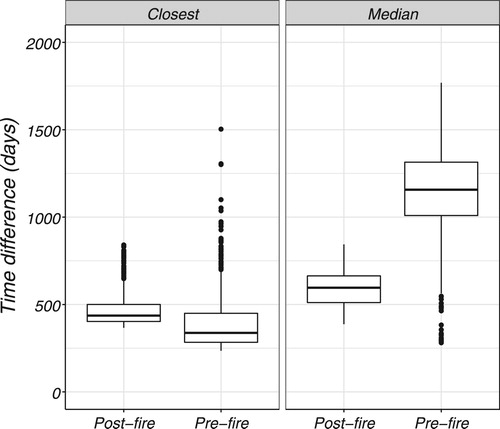
In total, we retrieved information from 1147 fire events covering 5.3 Mha. We extracted imagery from an area equivalent to 82 unique Landsat scenes (i.e. path and row combinations) and a total of 18,148 pre- and post-fire images. On average a pre-fire pixel had 21 Landsat observations in the 6 years prior to the fire, of which 9 were usable after filtering for noise and cloud (Figure 4). The closest pre-fire observation occurred an average of 41 days from the opening of the acquisition window, or 323 days before the fire (Figure 5). In contrast, a post-fire pixel had an average of eight Landsat observations over the two-year observation window, of which an average of three was usable after filtering out potentially noisy pixels (Figure 4). The closest post-fire observation was acquired an average of 104 days after the acquisition window opened, or 386 days after the fire event (assuming that each fire occurred on the 1st of August). The median value selected for the post-fire window across all fire events was on average 230 days after the window opened (126 days since the first acquisition), or 512 days from the fire date (Figure 5). The median value selected for the pre-fire composite was acquired in average 772 days since the opening of the pre-fire window (731 days from the closest acquisition), or an average of 1137 days before the fire.

Figure 4. Number of observations per pixel for the image compositing averaged by individual fires.

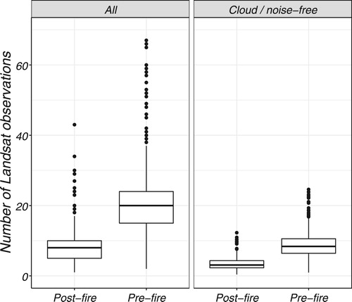
Figure 5. Time difference (days) for the image compositing averaged by individual fires.

Notes: ‘Median’ corresponds the distance in days between the selected median pixel and a hypothetical fire occurring the 1st of August of the fire year reported in the fire history databases. ‘Closest’ is the nearest observation in days from a hypothetical fire occurring the 1st of August of the fire year.

4.2. Secondary screening

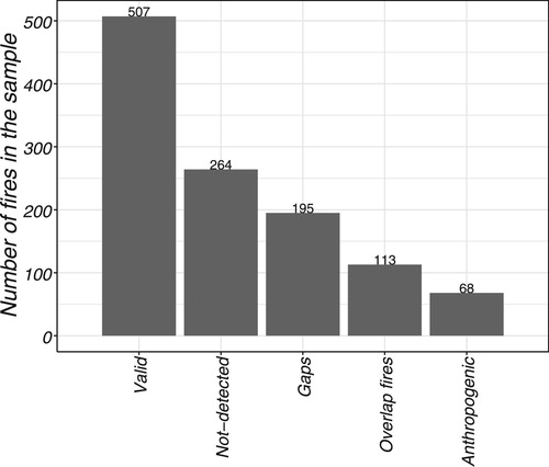
From the 1147 fires analysed 507 (44%) adhered to the secondary screening criteria (Figure 6). Of the 640 fires that were discarded at this step, 195 (17%) presented data gaps within the post-fire image composites making calculation of spatial landscape metrics impossible; 264 (23%) covered less than 30% of the reference perimeter area; 113 (10%) included adjacent/overlapping fire events; and 68 (7%) included anthropogenic disturbances (most often harvest cutblocks). The final sample included 507 fires ranging in size from 36 to 269,360 ha and covering 2,535,561 ha.

Figure 6. Summary of the screening process.

4.3. Spatial pattern analysis

4.3.1. Overall

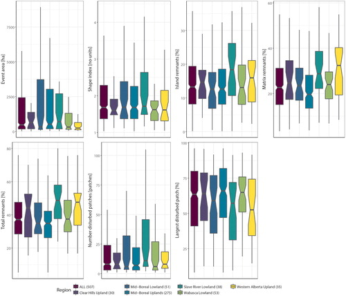
The event area (EA) ranged from 36 to 269,360 ha. The median EA of the fire sample was 475 ha, compared to a mean of 5001 ha indicating that fire size is highly positively skewed (Figure 7). In fact, the 9% of fires greater than 10,000 ha represent 75% of the area burned in all fires in the sample. The mean SI was 2.09, and 1.68 at the median, ranging from 1.03 to 12.23. The mean NDP was 52, with a median of 8, and a range from 1 to 3117. However, both the NDP and the SI co-varied directly with fire size, where the NDP ranged between averages of 7 and 421, and the SI between 1.6 and 5, for fires smaller than 1000 and 421 and 5.0 for fires greater than 10,000 ha. The %LDP averaged 60% and was 63% at the median, with a range from 8% to 96%. The %TR, %IR and %MR had means of 39%, 15% and 24%, respectively; and medians of 37%, 13% and 23%, respectively. %TR ranged from 5% to 91%, IR from 1% to 56% and MR from 3% to 59%.

Figure 7. Summary boxplots of the comparison between ecoregions.

4.3.2. Ecoregions comparison

We found significant differences in fire patterns for four of the seven metrics in four ecoregion pairs (Figure 8). The %MR of the Mid-Boreal Uplands (MBU) were significantly lower than those from the Western Alberta Upland (WAU), Slave River Lowland (SRL) or Wabasca Lowland (WL) ecoregions. In addition, the %TR of the MBU were significantly lower than those from the WAU or SRL ecoregions. The fires in MBU had significantly lower IR than those from SRL and significantly larger EA than those in WAU. We also observed large differences in the median values through the spyder plots (Figure 8) that did not translate into significant differences as captured by the KS and WX analyses. An example is the comparatively larger size of the fires in SRL relative to other ecoregions (Figure 8). This suggests that some of these differences may be the result of differences in the population shape that are not necessarily associated with shifts in median values. Some of the least represented ecoregions might not show significant differences due to lack of statistical power as a result of small sample sizes and the conservative .01 significance values we used.

Figure 8. Spyder plot grouped by fire pattern metric and significant differences in the cumulative distribution functions by ecoregion pairs (in box).

Notes: The spyder plots are calculated using the median of each metric. The maximum and minimum values for each metric correspond to the maximum and minimum ecoregion values for each metric. EA is event area; SI is the shape index; %TR is the percentage of remnant islands; %IR is percentage of island remnants; %MR is the percentage of matrix remnants; NDP is the number of disturbed patches; and %LDP is the percentage of the largest disturbed patch. ALL stands for all fires combined; MBU for Mid-Boreal Uplands; WL for Wabasca Lowland; MBL for Mid-Boreal Lowlands; SRL for Slave River Lowlands; WAU for Western Alberta Uplands; and CHU for Clear Hills Uplands. The significant differences by the combination of WX and the KS tests at the .01 significance are represented in the box at the right hand side.

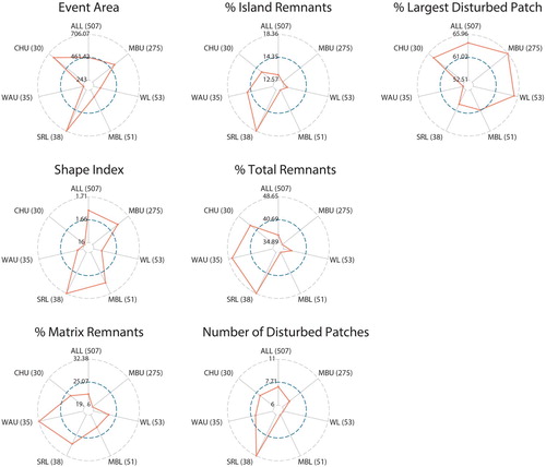
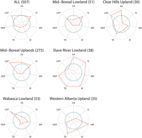
The spyder plots grouped by ecoregion (Figure 9) highlighted unique combinations of fire pattern metrics suggesting the existence of unique ‘signatures’ of burning patterns in the areas of study. Two groups of fire patterns were particularly easily differentiated. The SRL group had much larger fires (+EA), with more complex shapes (+SI); a higher amount of disturbed patches (+NDP) but a relatively small largest patch area (−%LDP) relative to other regions. The SRL region also had a higher amount of vegetation residuals than the other ecoregions (+%TR, +%IR and +%MR). In contrast, fires in the WL region were smaller, had more regular shapes (−SI), fewer disturbed patches (−NDP), a more important contribution of the largest patch area (+%LDP), and less residual vegetation (−%IR and −%MR). The rest of ecoregions presented more complex, and less distinctive fire pattern characteristics. MBL was characterized by smaller-sized fires (−EA), above-average fire event complexity (+SI), few disturbed patches (−NDP) with no clear dominant patch in terms of total area (−%LDP), and a below average amount of residuals (−%IR and −%MR). MBU had close to average size and complexity (∼EA and ∼SI), below average NDP (−NDP), a more dominant largest patch (+%LDP) and much smaller level of all types of residuals (−%IR and −%MR). Lastly, CHL had very large fires (+EA) that are simply shaped (−SI), with an average amount of disturbed patches, one large dominant disturbed patch (+%LDP), and an average amount of overall residuals (∼%IR and ∼%MR). WAU had very small fires (−EA) with simple shapes (−SI), a smaller than average amount of disturbed patches (−NDP) and a relatively small contribution of the largest patch area (−%LDP). The amount of residuals lying entirely within disturbed patches in the WAU was average (∼%IR), although it had the highest amount of residuals physically attached to the intact forest (+%MR).

Figure 9. Spyder plot by ecoregion.

Notes: The spyder plots are calculated using the median of each metric. The maximum and minimum values for each metric correspond to the maximum and minimum ecoregion values for each metric. EA is event area; SI is the shape index; %TR is the percentage of remnant islands; %IR is the percentage of island remnants; %MR is the percentage of matrix remnants; NDP is the number of disturbed patches; and %LDP is the percentage of the largest disturbed patch.

5. Discussion

5.1. Image selection, processing and secondary screening

One of the advantages of using Landsat data to capture wildfire patterns is access to significantly more fires across a greater area – relative to an approach based on aerial photo-interpretation (API). The results from 507 fires in our dataset certainly suggest that this is true. Extrapolating from the effort required to assemble the 129 fire database in the western boreal (from Andison and McCleary 2014), it would take years, and several millions of dollars to build a database of more than 500 fires using aerial photos.

Having said that, one of the limitations of the method proposed here is the ineligibility of a substantial number of fires. The primary limitation of any method that uses Landsat data is that it is limited to capturing fire patterns post-1985 – as Landsat TM imagery was only systematically collected after 1984 (White and Wulder 2014). This potentially creates a temporal bias since it eliminates as much as 50 years of otherwise available fire history, depending on the location. The pre-1985 period is relevant because it not only includes significantly different climate patterns, but also most the only pre-suppression fire data for the southern boreal. This could be an important limitation for studies with the goal of creating benchmarks for forest management. If the only available fire data in a given region are from the post-fire control era, while the technique proposed here could be applied, the raw data used to develop the metrics will be biased. For studies further north where fire control is either more recent, or has not yet occurred, this is not an issue (e.g. Burton et al. 2008).

Of the 1147 fires from the fire databases that occurred after 1985 and were larger than 100 ha in size, 17% were discarded as a result of data gaps. To increase the amount of available pixels after the filtering, the distance used to discard pixels near clouds could be decreased, or the tolerance to eliminate haze increased. It is not recommended to further extend the acquisition window because it can cause variability in Landsat spectral reflectance, in particular dNBR values, due to changes in phenology and sun elevation in northern regions (Verbyla, Kasischke, and Hoy 2008).

Another 23% of the fires were eliminated because the fire perimeters from the fire databases did not overlap sufficiently with the fire perimeter detected using the Landsat-based approach. There are two possible reasons for this error. First, the historical fire databases fail to accurately capture the outer boundaries of some historical wildfires due to errors in spatial location and/or date of fire occurrence. If true, this could be a serious limitation for any spatial analyses that includes pre-fire conditions, topographic features, or fuel type, and may be worth further investigation. A second possible reason for the significant difference in fire boundary delineation is the presence of wetlands. By comparing those fires with EOSD land cover product (Wulder et al. 2007) we observed that many of these fires were dominated by non-treed wetlands and presented strong negative dNBR signals suggesting greener and moister post-fire scenarios indicative of vegetation regrowth (Pereira et al. 1999). This ‘wetter’ post-fire scenario was also identified by Jones et al. (2013) as a challenge for mapping fire pattern in wetlands in the Everglades of Florida. The authors hypothesized that fire affected patch soils and elevation leading to higher water tables. The results suggest that it is difficult to capture changes over areas that regenerate quickly after fire using this method, as imagery of the fire year is not utilized. To maximize the quality of the results using this framework we suggest using the EOSD product to discard fires dominated by those vegetation types. Unfortunately, this creates a biased sample. Methods such as proposed by Hermosilla et al. (2016) that identify and characterize the NBR magnitude drop after disturbance based on imagery from the fire year might be more suitable to capture burned areas in non-treed wetlands. Our experience also suggests that those parts of fires that burn in wetlands are readily identified by manual interpretation through differentiating standing dead trees with an understory of lush green vegetation.

Fires were also deemed ineligible because they included overlapping neighbouring fires (10%) or cultural features (7%) that inflated the perimeters and thus biased the fire pattern metrics. The overlapping fires must have occurred by the end of the pre-fire window (after the median value selected) or during the post-fire window but on a different year. The challenge, in this case, is differentiating the patterns from a single fire event in time and space. This is an unavoidable challenge, and applies equally to API sampling. Similarly, the choice of fire-size threshold (100 ha minimum in this case) is subjective, and thus also a universal filter regardless of the method used. To resolve this challenge a means of defining the fire perimeter prior to the analysis is necessary. This could be undertaken in an automated way as an integrated part of the process through spectral trend analysis as in Hermosilla et al. (2016); or manually through visual interpretation of dNBR values for single fires as in Monitoring Trends in Burn Severity project (MTBS) in USA (Eidenshink et al. 2007).

5.2. Spatial pattern analysis

5.2.1. Overall

The event sample was skewed towards smaller events, although most of the area burned was the result of infrequent events larger than 10,000 ha. This is consistent with findings from other studies focusing on larger areas of study and time frames using historical database data (e.g. Stocks et al. 2002), which suggests that our sample is consistent with the historical fire-size distribution.

In terms of general burn patterns, the two fire pattern metrics that varied by event size – the number of patches and the event shape – have been noted by others. The idea that larger fires have more complex shapes than smaller ones is not new and has been reported in multiple studies based on various data sources and methods for the same study area (Andison and McCleary 2014; Burton et al. 2008; Eberhart and Woodard 1987; Parisien et al. 2006). However, while our averaged shape values were similar to these other studies we found considerably higher values for the larger fires. The more convoluted perimeters obtained from the pixel-based mortality maps were likely the result of an increased presence of peninsulas and bays in a pixelated format compared to the more generalized shapes coming from the aerial photo-interpretation process. These differences highlight the need to characterize detailed fire patterns using standardized methods and a consistent spatial language (sensu Andison 2012).

The increase in the NDP with event size was also identified by Andison and McCleary (2014), which was the only other study to report this particular metric. We found that fire events had a dominant disturbance patch covering 40–80% (second and third quartiles) of total area, which almost exactly matches the pattern noted by Andison and McCleary (2014).

With regards to the amount of residuals, the 37% reported in this manuscript is close to the 41% calculated by Andison and McCleary (2014) for the same area using the same spatial language and aerial photo-interpretation. It is also within the 20–40% reported by Soverel, Perrakis, and Coops (2010) for fires in western boreal Canada. Our results are however substantially higher than the 3–15% of Delong and Tanner (1996) in northeastern British Columbia, which we attribute to spatial language differences. Their definition of ‘residuals’ (averaging 9%) was the equivalent of our ‘island remnants’, which in this study averaged 13%. The vast majority of the remaining 28% difference exists in remnant area reflects the inclusion of ‘matrix remnants’, for which Delong and Tanner (1996) did not account.

5.2.2. Ecoregions comparison

The comparison between ecoregions revealed differences in fire metrics that suggest differences in dominant weather patterns, topography and vegetation patterns that affect fire behaviour (Ryan 2002). The most telling result was the higher amount of residuals in wildfires of the MBU compared to those of both the WAU and SRL. The differences between the MBU and the SRL are logically consistent with differences in moisture content, the physical arrangement of the fuels, climate and topography. The MBU has a larger proportion of flammable fuel types compared to SRL and less fragmentation (Parisien et al. 2004). SRL has colder temperatures, sparser vegetation and a comparatively higher amount of peatlands, fens and bogs than MBU (Ecological Stratification Working Group 1996). Although the SRL is dominated by more flammable conifer fuel types, it is distributed sparsely in exposed, waterlogged or non-productive areas that reduces fuel continuity and overall fuel loads, which in turn decreases overall fire intensity and increases the chances of residual formation (e.g. Harper et al. 2004). The fact that fire is less likely to burn in wetlands areas or with high moisture regime, creating pockets of remnants (Araya, Remmel, and Perera 2016; Epting, Verbyla, and Sorbel 2005; Leduc, Bergeron, and Gauthier 2007; Nowak, Kershaw, and Kershaw 2002) further supports this hypothesis.

Similarly, the differences between MBU and WAU are consistent with changes in topography that control the soil moisture regime and the fuel accumulation. The southern part of the WAU ecoregion (where most fires are) extends into the Rocky mountain foothills, and is dominated by linear ridges with strong local relief. Local topography is known to influence fire behaviour and residual formation. For example, slope changes and ridges have been associated with fire boundaries (Holsinger, Parks, and Miller 2016) and strong topographic variation is known to control fuel accumulation and moisture, which ultimately increases the chances of residual formation (Kane et al. 2015; Krawchuk et al. 2016).

Details aside, the ecoregion differences noted here strongly suggest that fire signature patterns are in fact linked to broad differences in vegetation, topography and climate patterns. The ability to capture and understand the specifics of such patterns is a key to not just fire behaviour prediction, but a better representation of pre-industrial conditions for harvest pattern emulation efforts. Lastly, the results also suggest that assuming that fire pattern signatures translate from one ecological zone to the next would be inadvisable.

6. Conclusion

Understanding pre-industrial wildfire patterns, in particular analysed residual patterns and/or partial mortality, has become both a research and forest management priority in Canada and beyond (Perera 2014). Over the last two decades, we have learned just how challenging it is to create this knowledge in a defendable manner. Importantly, we have learned that natural wildfire patterns have a very high level of natural variability (e.g. Andison and McCleary 2014; Parisien et al. 2006), which makes studies with small sample sizes, limited geographic scope, or biased data interesting, but not particularly valuable. Free and open access to the Landsat archive has enabled the detection and delineation of an unprecedented number of fire events across the boreal forest (White et al. 2017; Wulder and Coops 2014), and thus has potential to help unify a growing collection of fire pattern data into comprehensive databases. However, to-date Landsat-based studies on boreal fire patterns are either not accurate enough, do not include partial mortality (which we now believe to be a critical part of historic patterns) and/or based on a very small number of fires. Moreover, they all differ in their methods, data and spatial language (sensu Andison 2012). However, while fire mortality maps generated from aerial photo-interpretation are highly accurate and precise, the cost is high, and it can only be undertaken in areas where sufficient coverage of aerial photos exists (Morgan, Gergel, and Coops 2010).

Similarly, CBI (Key and Benson 2006) field plots are used to calibrate burn severity maps from freely available Landsat data, but they are very expensive to collect, variable among observers and lacking a clear agreed-upon biometric definition (Kolden, Matthew, and Smith 2016); of all which hinder applicability of the method to large scales and makes difficult to compare and interpret the results. In all, this makes it difficult for managers and other researchers alike to interpret fire patterns over both small areas (because one cannot be sure that small studies captured the variability of fire patterns) and larger areas (because the data, methods and assumptions from different studies are not comparable). What is needed is a universal combination of data sources, methods and spatial language that can be applied to generate a large enough sample size – of sufficient accuracy – to differentiate the signature of within zone fire patterns from those between zones.

Our contribution to this challenge was to test the ability of Landsat imagery to capture and compare fire patterns using a repeatable, consistent and cost-effective approach to a sufficient degree of accuracy and completion across the boreal biome. The proposed framework represents an example of what that may look like. The framework utilizes a recently developed fire mapping approach by San-Miguel, Andison, and Coops (2017) that essentially replaces our reliance on very expensive, subjective, and arguably inappropriate CBI data with less expensive, highly accurate, and very specific API data to both calibrate and validate a simple tree mortality maps.

Our model consists of supervised RF classification of freely available Landsat data and tree mortality polygons from aerial photo-interpretation to produce three-class mortality maps, which, after aggregated in discrete events using the spatial language proposed by Andison (2012), are used to calculate seven key fire pattern metrics. The framework requires basic reference information from fire databases: (1) a reference perimeter, to define the area of interest for each fire; and (2) the year of fire occurrence, to determine the pre- and post-fire images needed for the analysis. We demonstrated this methodological framework by mapping and characterizing key fire patterns characteristics for 507 events across the BP ecozone. Thus, although this model does not require field-based data such as that from CBI plots, it does require a sample of representative mortality maps generated from API for each new region to which it is calibrated.

Landsat imagery is an invaluable resource for mapping boreal wildfires using the proposed framework. Despite our rigorous screening process, we were able to include over 500 fires in our sample – far in excess of any other study to date for the study area. The results suggest that there is indeed value in capturing and comparing fire pattern signatures between and within broad ecological zones. Summaries from this demonstration generated a significant amount of new information on the fire pattern signature of various ecoregions of the BP ecozone that is critically required by managers. The comparison between ecoregions revealed differences in fire metrics, which in turn suggested various climate, topography and/or vegetation ecosystem drivers.

Despite the many virtues of Landsat data and our methods as described here, this study revealed three critical limitations. First, given our understanding of the strong link between fire weather and burning patterns (e.g. Macias Fauria and Johnson 2008; Wotton, Nock, and Flannigan 2010), limiting fire pattern data to 1985 and beyond almost certainly compromises our ability to capture the full range of fire patterns. This also introduces a strong fire control bias of the forest management areas where fire control has been in effect since 1985. The second limitation is that this study revealed a potential key weakness of Landsat data as regards identifying fire patterns in wetlands. The spectral signature of vegetation regrowth in such areas is difficult to identify by anything other than subjective means via photo-interpretation. It is also important to note that applying the methods described in this paper to another major ecological region requires aerial photo-interpreted data for calibration. Thus, the third limitation of this study is that the model still requires a sample of fire mortality maps generated from aerial photos, for both calibration and validation. However, the number of fires required to capture the variability of fire patterns is still far less that what would be required using plot data.

Overall, the results suggest that our original hypothesis that the Landsat data archive can be used to accurately and universally provide precise historical fire patterns is partially, but not entirely proven to be true. If the goal is to create highly defendable fire pattern results across and between areas of the boreal forest, our results suggest that some combination of Landsat and aerial photo-based data and methods are required.

Acknowledgements

This research project is a part of the Healthy Landscapes Program of fRI Research. We would like to thank Dr Txomin Hermosilla who provided insight and expertise that greatly assisted the research, and to Dr Mike Wulder and collaborators for facilitating access to fire change information (https://opendata.nfis.org/mapserver/nfis-change_eng.html). We would also like to show our gratitude to Saskatchewan Ministry of Environment, the government of the Northwest Territories, Mistik Management, and Doug Turner, Chris Dallyn, Kathleen Gazey, Al Balisky, Cliff McLauchlan, Roger Nesdoly, Kim Rymer, and David Stevenson for making possible and sharing their wisdom during a field visit. Finally, we thank the editor and three anonymous reviewers for comments that greatly improved the manuscript.

Disclosure statement

No potential conflict of interest was reported by the authors.

ORCID

Ignacio San-Miguel http://orcid.org/0000-0001-8390-4723

Nicholas C. Coops http://orcid.org/0000-0002-0151-9037

Additional information

Funding

This research was made possible thanks to Saskatchewan Environment, fRI Research Healthy Landscapes Program, the government of the Northwest Territories, Bandaloop Landscape-Ecosystem Services, and an NSERC Discovery and Engage grant to Coops (RGPIN 311926-13 and EGP 503226-16).

References

- Andison, D. W. 2012. “The Influence of Wildfire Boundary Delineation on Our Understanding of Burning Patterns in the Alberta Foothills.” Canadian Journal of Forest Research 42: 1253–1263. doi:10.1139/x2012-074.
- Andison, D. W., and K. McCleary. 2014. “Detecting Regional Differences in Within-Wildfire Burn Patterns in Western Boreal Canada.” The Forestry Chronicle 90: 59–69. doi:10.5558/tfc2014-011.
- Araya, Y. H., T. K. Remmel, and A. H. Perera. 2016. “What Governs the Presence of Residual Vegetation in Boreal Wildfires?” Journal of Geographical Systems 18: 159–181. doi:10.1007/s10109-016-0227-9.
- Banks, S. C., M. Dujardin, L. Mcburney, D. Blair, M. Barker, and D. B. Lindenmayer. 2011. “Starting Points for Small Mammal Population Recovery After Wildfire : Recolonisation or Residual Populations?” Oikos 120: 26–37. doi:10.1111/j.1600-0706.2010.18765.x.
- Bolton, D. K., N. C. Coops, and M. A. Wulder. 2015. “Characterizing Residual Structure and Forest Recovery Following High-Severity Fire in the Western Boreal of Canada Using Landsat Time-Series and Airborne Lidar Data.” Remote Sensing of Environment 163: 48–60. doi:10.1016/j.rse.2015.03.004.
- Boucher, J., B. Beaudoin, C. Hebert, L. Guindon, and E. Bauce. 2017. “Assessing the Potential of the Differenced Normalized Burn Ratio (dNBR) for Estimating Burn Severity in Eastern Canadian Boreal Forests.” International Journal of Wildland Fire 26: 32–45. doi:10.1071/WF15122.
- Boulanger, Y., S. Gauthier, P. J. Burton, and M. -A. Vaillancourt. 2012. “An Alternative Fire Regime Zonation for Canada.” International Journal of Wildland Fire 21: 1052. doi:10.1071/WF11073.
- Boulanger, Y., S. Gauthier, D. R. Gray, H. Le Goff, P. Lefort, and J. Morissette. 2013. “Fire Regime Zonation Under Current and Future Climate Over Eastern Canada.” Ecological Applications 23: 904–923. doi:10.1890/12-0698.1.
- Brandt, J. 2009. “The Extent of the North American Boreal Zone.” Environmental Reviews 17: 101–161. doi:10.1139/A09-004.
- Breiman, L. 2001. “Random Forests.” Machine Learning 45: 5–32. doi:10.1023/A:1010933404324.
- Burton, P. J., M.-A. Parisien, J. A. Hicke, R. J. Hall, and J. T. Freeburn. 2008. “Large Fires as Agents of Ecological Diversity in the North American Boreal Forest.” International Journal of Wildland Fire 17: 754–767. doi:10.1071/WF07149.
- Canadian Forest Service, 2013. “Canada’s National Forest Inventory, Revised 2006 Baseline.” Available online at https://nfi.nfis.org/.
- Christophe, E., J. Inglada, and A. Giros. 2008. “Orfeo Toolbox : a Complete Solution for Mapping from High Resolution Satellite.” Interantional Archives of the Photogrammetry, Remote Sensing and Spatial Information Sciences 36: 1263–1268.
- Cocke, A. E., P. Z. Fulé, and J. E. Crouse. 2005. “Comparison of Burn Severity Assessments Using Differenced Normalized Burn Ratio and Ground Data.” International Journal of Wildland Fire 14: 189. doi:10.1071/WF04010.
- Delong, S. C., and D. Tanner. 1996. “Managing the Pattern of Forest Harvest: Lessons from Wildfire.” Biodiversity and Conservation 5: 1191–1205. doi:10.1007/BF00051571.
- Eberhart, K. E., and P. M. Woodard. 1987. “Distribution of Residual Vegetation Associated with Large Fires in Alberta.” Canadian Journal of Forest Research 17: 1207–1212. doi: 10.1139/x87-186
- Ecological Stratification Working Group. 1996. “ A National Ecological Framework for Canada.”
- Eidenshink, J., B. Schwind, K. Brewer, Z. Zhu, B. Quayle, S. Howard, S. Falls, and S. Falls. 2007. “A Project for Monitoring Trends in Burn Severity.” Fire Ecology 3: 3–21. doi: 10.4996/fireecology.0301003
- Epting, J., D. Verbyla, and B. Sorbel. 2005. “Evaluation of Remotely Sensed Indices for Assessing Burn Severity in Interior Alaska Using Landsat TM and ETM+.” Remote Sensing of Environment 96: 328–339. doi:10.1016/j.rse.2005.03.002.
- Fraser, R. H., J. van der Sluijs, and R. J. Hall. 2017. “Calibrating Satellite-Based Indices of Burn Severity from UAV-derived Metrics of a Burned Boreal Forest in NWT, Canada.” Remote Sensing. doi:10.3390/rs9030279.
- French, N. H. F., E. S. Kasischke, R. J. Hall, K. A. Murphy, D. L. Verbyla, E. E. Hoy, and J. L. Allen. 2008. “Using Landsat Data to Assess Fire and Burn Severity in the North American Boreal Forest Region: An Overview and Summary of Results.” International Journal of Wildland Fire 17: 443. doi:10.1071/WF08007.
- García, M. J. L., and V. Caselles. 1991. “Mapping Burns and Natural Reforestation Using Thematic Mapper Data.” Geocarto International 6: 31–37. doi:10.1080/10106049109354290.
- Hall, R. J., J. T. Freeburn, W. J. de Groot, J. M. Pritchard, T. J. Lynham, and R. Landry. 2008. “Remote Sensing of Burn Severity: Experience from Western Canada Boreal Fires.” International Journal of Wildland Fire 17: 476. doi:10.1071/WF08013.
- Harper, K. A., D. Lesieur, Y. Bergeron, and P. Drapeau. 2004. “Forest Structure and Composition at Young Fire and cut Edges in Black Spruce Boreal Forest.” Canadian Journal of Forest Research 34: 289–302. doi:10.1139/x03-279.
- Hermosilla, T., M. A. Wulder, J. C. White, N. C. Coops, G. W. Hobart, and L. B. Campbell. 2016. “Mass Data Processing of Time Series Landsat Imagery: Pixels to Data Products for Forest Monitoring.” International Journal of Digital Earth 8947: 1–20. doi:10.1080/17538947.2016.1187673.
- Holsinger, L., S. A. Parks, and C. Miller. 2016. “Weather, Fuels, and Topography Impede Wildland Fire Spread in Western US Landscapes.” Forest Ecology and Management 380: 59–69. doi:10.1016/j.foreco.2016.08.035.
- Hunter, M. L. H. 1993. “Natural Fire Regimes as Spatial Models for Managing Boreal Forests.” Biological Conservation 65: 115–120. doi:10.1016/0006-3207(93)90440-C.
- Jones, J. W., A. E. Hall, A. M. Foster, and T. J. Smith. 2013. “Wetland Fire Scar Monitoring and Analysis using Archival Landsat Data for the Everglades.” Fire Ecology 9, 133–150. doi:10.4996/fireecology.0901133.
- Kane, V. R., J. A. Lutz, C. Alina Cansler, N. A. Povak, D. J. Churchill, D. F. Smith, J. T. Kane, and M. P. North. 2015. “Water Balance and Topography Predict Fire and Forest Structure Patterns.” Forest Ecology and Management 338: 1–13. doi:10.1016/j.foreco.2014.10.038.
- Kennedy, R. E., Z. Yang, and W. B. Cohen. 2010. “Detecting Trends in Forest Disturbance and Recovery Using Yearly Landsat Time Series: 1. LandTrendr—Temporal Segmentation Algorithms.” Remote Sensing of Environment 114: 2897–2910. doi:10.1016/j.rse.2010.07.008.
- Key, C. H., and N. C. Benson. 2006. “Landscape Assessment: Ground Measure of Severity, the Composite Burn Index, and Remote Sensing of Severity, the Normalized Burn Index.” In FIREMON: Fire Effects Monitoring and Inventory System, edited by D. C. Lutes, R. E. Keane, J. F. Caratti, C. H. Key, N. C. Benson, S. Sutherland, and L. J. Gangi. Ogden, UT: USDA Forest Service, Rocky Mountain Research Station, General Technical Report RMRS-GTR-164-CD: LA1–51.
- Kolden, C., A. Matthew, and S. Smith. 2016. “Limitations and Utilization of Monitoring Trends in Burn Severity products for assessing Wildfire Severity in the USA.” doi:10.1071/WF15082.
- Krawchuk, M. A., S. L. Haire, J. Coop, M.-A. Parisien, E. Whitman, G. Chong, and C. Miller. 2016. “Topographic and Fire Weather Controls of Fire Refugia in Forested Ecosystems of Northwestern North America.” Ecosphere (Washington, D.C.) 7. doi:10.1002/ecs2.1632.
- Landres, P. B., P. Morgan, and F. J. Swanson. 1999. “Overview of the Use of Natural Variability Concepts in Managing Ecological Systems.” Ecological Applications 9: 1179–1188. doi:10.1890/1051-0761(1999)009[1179:OOTUON]2.0.CO;2.
- Leduc, A., Y. Bergeron, and S. Gauthier. 2007. “Relationships Between Prefire Composition, Fire Impact, and Post-fire Legacies in the Boreal Forest of Eastern Canada.” In The Fire Environment: Innovations, Management, and Policy, edited by B. W. Butler, and W. Cook, 187–193. Fort Collins, CO: USDA Forest Service, Rocky Mountain Research Station, Proceedings RMRS-p-46CD.
- Lentile, L. B., Z. a. Holden, A. M. S. Smith, M. J. Falkowski, A. T. Hudak, P. Morgan, S. a. Lewis, P. E. Gessler, and N. C. Benson. 2006. “Remote Sensing Techniques to Assess Active Fire Characteristics and Post-fire Effects.” International Journal of Wildland Fire 15: 319–345. doi: 10.1071/WF05097
- Loehman, R. A., E. Reinhardt, and K. L. Riley. 2014. “Wildland Fire Emissions, Carbon, and Climate: Seeing the Forest and the Trees – A Cross-Scale Assessment of Wildfire and Carbon Dynamics in Fire-Prone, Forested Ecosystems.” Forest Ecology and Management 317: 9–19. doi:10.1016/j.foreco.2013.04.014.
- Macias Fauria, M., and E. A. Johnson. 2008. “Climate and Wildfires in the North American Boreal Forest.” Philosophical Transactions of the Royal Society B: Biological Sciences 363: 2315–2327. doi:10.1098/rstb.2007.2202.
- Madoui, A., A. Leduc, S. Gauthier, and Y. Bergeron. 2010. “Spatial Pattern Analyses of Post-Fire Residual Stands in the Black Spruce Boreal Forest of Western Quebec.” International Journal of Wildland Fire 19: 1110. doi:10.1071/WF10049.
- Mccarley, T. R., C. A. Kolden, N. M. Vaillant, A. T. Hudak, A. M. S. Smith, B. M. Wing, B. S. Kellogg, and J. Kreitler. 2017. “Multi-Temporal LiDAR and Landsat Quantification of Fire-Induced Changes to Forest Structure.” Remote Sensing of Environment 191: 419–432. doi:10.1016/j.rse.2016.12.022.
- Miller, J. D., and A. E. Thode. 2007. “Quantifying Burn Severity in a Heterogeneous Landscape with a Relative Version of the Delta Normalized Burn Ratio (dNBR).” Remote Sensing of Environment 109: 66–80. doi:10.1016/j.rse.2006.12.006.
- Morgan, J. L., and S. E. Gergel. 2010. “Quantifying Historic Landscape Heterogeneity from Aerial Photographs Using Object-Based Analysis.” Landscape Ecology 25: 985–998. doi:10.1007/s10980-010-9474-1.
- Morgan, J. L., S. E. Gergel, and N. C. Coops. 2010. “Aerial Photography: A Rapidly Evolving Tool for Ecological Management.” Bioscience 60: 47–59. doi:10.1525/bio.2010.60.1.9.
- Morgan, P., C. C. Hardy, T. W. Swetnam, M. Rollins, and D. Long. 2001. “Mapping Fire Regimes Across Time and Space: Understanding Coarse and Fine-Scale Fire Patterns.” International Journal of Wildland Fire 10: 329–342. doi: 10.1071/WF01032
- Nowak, S., G. P. Kershaw, and L. J. Kershaw. 2002. “Plant Diversity and Cover After Wildfire on Anthropogenically Disturbed and Undisturbed Sites in Subarctic Upland Picea Mariana Forest.” Arctic 55: 269–280. doi: 10.14430/arctic710
- Oliver, C. D. 1980. “Forest Development in North America Following Major Disturbances.” Forest Ecology and Management 3: 153–168. doi:10.1016/0378-1127(80)90013-4.
- OMNR (Ontario Ministry of Natural Resources). 2001. Forest Management Guide for Natural Disturbance Pattern Emulation (Version 3.1). Sault Ste. Marie, ON: Ontario Ministry of Natural Resources, Forest Management Branch.
- Parisien, M. A., K. G. Hirsch, S. G. Lavoie, J. B. Todd, and V. G. Kafka. 2004. Saskatchewan Fire Regime Analysis. Edmonton, AB: Canadian Forest Service Information Report NOR-X-194.
- Parisien, M., V. S. Peters, Y. Wang, J. M. Little, E. M. Bosch, and B. J. Stocks. 2006. “Spatial Patterns of Forest Fires in Canada, 1980–1999.” International Journal of Wildland Fire 15: 361–374. doi:10.1071/WF06009.
- Pereira, J., A. Sa, A. Sousa, J. Silva, T. Santos, and J. Carreiras. 1999. “Spectral Characterisation and Discrimination of Burnt Areas.” In Remote Sensing of Large Wildfires in the European Mediterranean Basin. doi:10.1007/978-3-642-60164-4.
- Perera, A. H. 2014. Ecology of Wildfire Residuals in Boreal Forests. New Jersey: Wiley. doi:10.1002/9781118870488.
- Pickell, P. D., D. W. Andison, and N. C. Coops. 2013. “Characterizations of Anthropogenic Disturbance Patterns in the Mixedwood Boreal Forest of Alberta, Canada.” Forest Ecology and Management 304: 243–253. doi: 10.1016/j.foreco.2013.04.031
- Rouse, J. W., R. H. Haas, D. W. Deerling, J. A. Schell, and J. C. Harlan. 1974. Monitoring the Vernal Advancement and Retrogradation (Green Wave Effect) of Natural Vegetation. Greenbelt, MD: NASA/ GSFC Type III Final Report.
- Ryan, K. C. 2002. “Dynamic Interactions Between Forest Structure and Fire Behavior in Boreal Ecosystems.” Silva Fennica 36: 13–39. doi:10.14214/sf.548.
- San-Miguel, I., D. W. Andison, and N. C. Coops. 2017. “Characterizing Historical Fire Patterns as a Guide for Harvesting Planning Using Landscape Metrics Derived from Long Term Satellite Imagery.” Forest Ecology and Management 399: 155–165. doi:10.1016/j.foreco.2017.05.021.
- Soverel, N. O., D. D. B. Perrakis, and N. C. Coops. 2010. “Estimating Burn Severity from Landsat dNBR and RdNBR Indices Across Western Canada.” Remote Sensing of Environment 114: 1896–1909. doi:10.1016/j.rse.2010.03.013.
- Stocks, B. J., J. A. Mason, J. B. Todd, E. M. Bosch, B. M. Wotton, B. D. Amiro, M. D. Flannigan, et al. 2002. “Large Forest Fires in Canada, 1959–1997.” Journal of Geophysical Research 108: 512. doi:10.1029/2001JD000484.
- Verbyla, D. L., E. S. Kasischke, and E. E. Hoy. 2008. “Seasonal and Topographic Effects on Estimating Fire Severity from Landsat TM/ETM+ Data.” International Journal of Wildland Fire 17: 527–534. doi: 10.1071/WF08038
- White, J. C., and M. A. Wulder. 2014. “The Landsat Observation Record of Canada: 1972–2012.” Canadian Journal of Remote Sensing 39: 455–467. doi: 10.5589/m13-053
- White, J. C., M. A. Wulder, T. Hermosilla, N. C. Coops, and G. W. Hobart. 2017. “A Nationwide Annual Characterization of 25 Years of Forest Disturbance and Recovery for Canada Using Landsat Time Series.” Remote Sensing of Environment 194: 303–321. doi:10.1016/j.rse.2017.03.035.
- White, J. C., M. A. Wulder, G. W. Hobart, J. E. Luther, T. Hermosilla, P. Griffiths, N. C. Coops, et al. 2014. “Pixel-Based Image Compositing for Large-Area Dense Time Series Applications and Science.” Canadian Journal of Remote Sensing 40: 192–212. doi:10.1080/07038992.2014.945827.
- Wiken, E. B. (comp.). 1986. Terrestrial Ecozones of Canada. Ecological Land Classification Series No. 19. Environment Canada, Hull, QC. 26 p. + map.
- Wilson, M. F. J., B. O. Connell, J. C. Guinan, and A. J. Grehan. 2007. “Multiscale Terrain Analysis of Multibeam Bathymetry Data for Habitat Mapping on the Continental Slope.” Marine Geodesy. doi:10.1080/01490410701295962.
- Woodcock, C. E., R. Allen, M. Anderson, A. Belward, R. Bindschadler, W. Cohen, F. Gao, et al. 2008. “Free Access to Landsat Imagery.” Science 320: 1011–1012. doi:10.1126/science.320.5879.1011a.
- Wotton, B. M., C. A. Nock, and M. D. Flannigan. 2010. “Forest Fire Occurrence and Climate Change in Canada.” International Journal of Wildland Fire 19: 253–271. doi: 10.1071/WF09002
- Wulder, M. A. 1998. “Optical Remote-Sensing Techniques for the Assessment of Forest Inventory and Biophysical Parameters.” Progress in Physical Geography 22: 449–476. doi:10.1191/030913398675385488
- Wulder, M. A., and N. C. Coops. 2014. “Satellites: Make Earth Observations Open Access.” Nature 513 (7516): 30–31. doi: 10.1038/513030a
- Wulder, M. A., J. C. White, S. N. Goward, J. G. Masek, J. R. Irons, M. Herold, W. B. Cohen, T. R. Loveland, and C. E. Woodcock. 2008. “Landsat Continuity: Issues and Opportunities for Land Cover Monitoring.” Remote Sensing of Environment 112: 955–969. doi:10.1016/j.rse.2007.07.004.
- Wulder, M. A., J. C. White, S. Magnussen, and S. McDonald. 2007. “Validation of a Large Area Land Cover Product Using Purpose-Acquired Airborne Video.” Remote Sensing of Environment 106: 480–491. doi:10.1016/j.rse.2006.09.012.
- Zhu, Z., and C. E. Woodcock. 2012. “Object-Based Cloud and Cloud Shadow Detection in Landsat Imagery.” Remote Sensing of Environment 118: 83–94. doi:10.1016/j.rse.2011.10.028.
- Zhu, Z., and C. E. Woodcock. 2014. “Continuous Change Detection and Classification of Land Cover Using all Available Landsat Data.” Remote Sensing of Environment 144: 152–171. doi:10.1016/j.rse.2014.01.011.