Urbanization between compactness and dispersion: designing a spatial model for measuring 2D binary settlement landscape configurations

ABSTRACT

Measuring spatial patterns is a crucial task in spatial sciences. Multiple indicators have been developed to measure patterns in a quantitative manner. However, most comparative studies rely on relative comparisons, limiting their explanatory power to specific case studies. Motivated by advancements in earth observation providing unprecedented resolutions of settlement patterns, this paper suggests a measurement technique for spatial patterns to overcome the limits of relative comparisons. We design a model spanning a feature space based on two metrics – largest patch index and number of patches. The feature space is defined as ‘dispersion index’ and covers the entire spectrum of possible two-dimensional binary (settlement) patterns. The model configuration allows for an unambiguous ranking of each possible pattern with respect to spatial dispersion. As spatial resolutions of input data as well as selected areas of interest influence measurement results, we test dependencies within the model. Beyond, common other spatial metrics are selected for testing whether they allow unambiguous rankings. For scenarios, we apply the model to artificially generated patterns representing all possible configurations as well as to real-world settlement classifications differing in growth dynamics and patterns.

KEYWORDS:

• Land cover
• spatial patterns
• landscape metrics
• dispersion index
• sensitivity analysis
• urban settlements
• remote sensing
• comparative spatial analysis

1. Introduction

Is the arrangement of artifacts in urban spaces concentrated or dispersed? While this frequently asked question seems to allow for a simple intuitive answer (‘you know it when you see it’), an objective measurement of spatial patterns or their comparison across space is not trivial. In the urban research domain, a multitude of elements can constitute morphological patterns depending on the particular scale, from individual objects such as buildings to aggregated thematic patches of (urban) land use at city levels. However, it is not explicitly agreed upon which spatial dimensions (scale, units of measurement) and which thematic features allow for a suitable characterization and representation of urban spatial patterns. As a consequence, the debate on the shape of spatial urbanization includes a confusing variety of theories, conceptual approaches, data sources and techniques for measurement applied to varying (land use-related) objects across different spatial scales of observation (e.g. Batty 2008; Esch et al. 2014; Siedentop and Fina 2012; Galster et al. 2001; Jabareen 2006; Tsai 2005). Critics claim that much of the work in the past can be contested due to a data-driven approach and a rather arbitrary use of metrics, scales of observation, spatial reference systems and geographical boundaries (e.g. Lechner et al. 2013; Riitters et al. 1995).

The debate on the appropriate means of analyzing urban land use (or land cover) patterns and their change over time is far from being only academic. National and supra-national institutions have underlined the importance of land use for a sustainable urban future (EEA/FOEN 2016; OECD 2010, 2012; SRU 2016; UN-Habitat 2009). Claims for more ‘compact’, less land consumptive (‘sprawling’) urban development are based on the empirically proven influence of land use patterns and urban form on energy consumption (Brownstone and Golob 2009; LSE Cities 2014; Silva, Oliveira, and Leal 2017), infrastructure efficiency (Burchell and Mukherji 2003) and landscape quality (Antrop 2004). Empirical studies have shown that spatial compactness – measured with different approaches and variables – is negatively associated with energy consumption, greenhouse gas emissions (Brownstone and Golob 2009; Ewing and Rong 2008; Newman and Kenworthy 2006; Stone et al. 2007), and public service costs (Burchell et al. 2005; Hortas-Rico and Solé-Ollé 2010; Speir and Stephenson 2002) as well as the loss of natural soils and habitat quality (Cieslewicz 2002; Jaeger and Schwick 2014; Theobald, Miller, and Thompson Hobbs 1997).

In contrast, in both the Global North and South, urban land use change has been described as a continuous transformation from formerly compact, concentrated land use patterns into spatially extended and morphologically less clear-cut urban configurations (Anas, Arnott, and Small 1998; Angel et al. 2011; Batty et al. 2004; Siedentop 2015; Siedentop and Fina 2010; Taubenböck et al. 2009, 2012). Most scholars argue that urban expansion has become edgeless, missing a concentration and simultaneously thinning out into fragmented peripheral areas (e.g. Angel and Blei 2016; Burger and Meijers 2012). A discontinuous and scattered spread of urban land uses into the surrounding areas of cities (‘leapfrogging’) has led to a highly complex pattern that is neither ‘urban’ nor ‘rural’ in character and is often referred to as ‘urban sprawl’ (EEA/FOEN 2016; Galster et al. 2001; Knaap et al. 2005; Siedentop 2005).

However, other researchers claim that urban sprawl might only be an intermediate phase of a long-term transition process leading to compact urban structures at higher scales (Peiser 1989, 2001). Following this line of thought, new development is filling in the leapfrogged, scattered territories along the urban periphery as the physical outcome of the former waves of suburbanization and urban expansion. What has formerly been portrayed as a ‘scattered’ or ‘discontinuous’ form of development will be contiguously urbanized and thus ‘compact’ at a higher spatial scale – at least in regions with ongoing socioeconomic growth pressures. Many scholars believe that ‘mega-urban’ structures in the shape of functionally connected and spatially merged networks and clusters of formerly individual cities represent the future of human habitats (Florida, Gulden, and Mellander 2008; Kraas and Mertins 2014; Lang and Knox 2009; Taubenböck et al. 2014; Taubenböck and Wiesner 2015).

Although a large body of literature regarding the means of analyzing urban spatial patterns exists, it is still challenging to empirically test claims related to their positive or negative effects. This is, on the one hand, due to the lack of consensus on how to empirically address urban land use and its change over time. On the other hand, this is due to the absence of time series data that would allow researchers to study the long-term trajectories of urban land use in appropriate geometric and thematic detail. Most empirical work is therefore restricted to a cross-sectional design or the analysis of recent trends of change. Studies vary due to different thematic variables, different scales and entities of measurement, or techniques of measurement applied. Regarding the scale of measurement, studies span from coarse perspectives on urban landscape classifications (e.g. Angel et al. 2011; Schneider and Woodcock 2008; Schneider, Chang, and Paulsen 2015) to highly detailed perspectives at the scale of individual buildings partly represented in three dimensions (e.g. Herold, Goldstein, and Clarke 2003; Seto and Fragkias 2005; Taubenböck et al. 2013; Wurm et al. 2014). Most studies focus on one single city or few cities (and metropolitan regions) of a single nation state (e.g. Galster et al. 2001; Herold, Goldstein, and Clarke 2003; Knaap et al. 2005; Luck and Wu 2002; Siedentop and Fina 2010; Zhang et al. 2004), whereas comparative studies across national boundaries are still rare (Angel 2012; Huang, Lu, and Sellers 2007; Seto and Fragkias 2005; Schneider and Woodcock 2008; Siedentop and Fina 2012; Taubenböck et al. 2017). Techniques that measure and evaluate spatial patterns range from simple approaches focusing on the extent of built-up areas to more sophisticated multidimensional analysis of shape and form characteristics (see EEA/FOEN [2016] for an overview).

In terms of the quantification of spatial urban patterns, a large body of literature applies the concept of landscape metrics, which originates from the field of landscape ecology (e.g. Bender, Tischendorf, and Fahrig 2003; McGarigal and Marks 1995; Schumaker 1996). It became popular to transfer these metrics onto the urban context in order to describe sizes, forms and spatial arrangements of urban land use (cover) configurations. Studies use these metrics, e.g. to identify gradients across space (e.g. Luck and Wu 2002; Zhang et al. 2004) or to relatively compare different city patterns across space and/or time (e.g. Herold, Goldstein, and Clarke 2003; Taubenböck et al. 2009) with assumptions regarding the effects of compactness, fragmentation or dispersion (e.g. Fragkias and Seto 2009).

We argue that the analysis of urban land use patterns will gain scientific importance in times of massive urbanization processes (UN 2016). While the above-mentioned metrics have demonstrated the ability to quantitatively describe distribution, size and forms of patches constituting the urban landscape, their application in the urban context is mostly based on assumptions. That is, there is no agreement among scholars as to what exactly defines compactness, fragmentation or dispersion; how these terms can be clearly conceptualized; which measures are decisive; and how they can be measured. Moreover, another critical point is that most previous studies evaluate urban patterns only relative to each other (e.g. ‘city A’ is more compact than ‘city B’ with respect to the specific metrics considered. However, whether ‘city A’ can be considered a compact city in relation to a larger statistical population is neglected). Therefore, studies based on relative comparisons among their specified sample limit their general transferability and explanatory power to case studies.

In this paper, it is our aim to suggest a model-based conceptualization for the evaluation of spatial patterns with respect to ‘compactness’ and ‘dispersion’. We base the work on a simplistic case of spatial patterns – two-dimensional patterns constituted by two thematic classes: ‘settlement’ and ‘non-settlement’. In doing so, we demonstrate that any two-dimensional pattern can be unambiguously ranked in relative, but also absolute terms between compact and dispersed layouts. We therefore consider ‘compactness’ and ‘dispersion’ as directions on the two ends of a continuum rather than fixed categories (Ewing and Hamidi 2015, 413; Johnson 2001, 719). Our model allows analyzing the incremental shift of urban landscapes from a state of relative compactness into a less regular, more dispersed spatial configuration or vice versa.

Beyond, as manifold spatial metrics have been developed for measuring patterns and arrangements, we test a selection of spatial metrics commonly used in other studies. The question here is whether these metrics can be unambiguously evaluated with respect to our model-based conceptualization of ‘dispersion’. And, as spatial extents and spatial resolutions of input data influence the evaluation of spatial patterns, we systematically test the sensitivity of the model onto respective variations. Finally, we exemplify the model capabilities using real-world examples. We base our example on a time series of binary settlement classifications (derived from multi-temporal earth observation (EO) data) from the 1970s until 2010.

Our motivation for this model-based conceptualization is also derived from recent advancements in remote sensing. New digital global settlement maps have recently been introduced at an unprecedented resolution (e.g. Esch et al. 2012; Pesaresi et al. 2013), with significantly improved accuracy (Klotz et al. 2016). With these new geodata in hand, this paper elaborates on new capabilities for consistent comparative analysis of spatial patterns across the globe. As a consequence, we lend our thematic and conceptual framework for this study from the field of urbanization, where scientific debates on spatial layout configurations alternate between the terms and concepts of compactness, sprawl, fragmentation and dispersion (e.g. Mubareka et al. 2011; Schneider and Woodcock 2008; Sudhira, Ramachandra, and Jagadish 2004).

The remainder of this paper is organized as follows. Section 2 introduces the conceptual foundation and the model design for measuring binary spatial patterns. In Section 3, we test the model and the dispersion index (DI) with artificially generated patterns. In Section 4, other commonly used spatial metrics are tested. Here, the validity of these metrics is analyzed whether an unambiguous evaluation of patterns within the model design is feasible. In Section 5, the influence of the model parameters ‘spatial extent’ and ‘spatial resolutions of input data’ are tested. In Section 6, we apply the model onto selected real-world settlement patterns. We measure the evolution of urban patterns classified from EO data over a time period of 35 years. This is followed by a discussion in Section 7, concluding with a perspective on the implications of the results.

2. Model design for measuring spatial landscape configurations: conceptual background, spatial metrics and DI

2.1. Conceptual foundation

Cities can be conceptualized in numerous ways. In general, for a given spatial entity, an almost unlimited number of spatial landscape configurations are possible. The complexity increases with the number of thematic classes and the geometric resolution. In this study, we reduce the complexity of urban patterns to a mere physical dimension. Beyond this, we consider only an aggregated description in the form of a two-dimensional representation of the built environment, operationalized as ‘settlement’ and ‘non-settlement’ areas.

With the generalized representation of the landscape, the number of possible spatial configurations is significantly reduced. Our binary classification of the landscape can be captured by the area coverage of the thematic class, the spatial distribution, and the size and shape of the patches. Patches, as the defining elements of the landscape, are understood as a single spatial entity (here a cell) or multiple adjacent contiguous entities (cells) of the same land cover class (Lang and Blaschke 2007).

The proposed model derives its conceptual motivation from the idea of measuring and evaluating spatial patterns according to the attributes ‘compaction’ (process) or ‘compact’ (state) and ‘dispersion’ or ‘dispersed’. These terms address the changing spatial distribution of urban functions across a given space from a process or static view. According to Schneider and Woodcock (2008), dispersion can be understood as the movement of urban functions outward from the urban core. Dispersed (urban) landscape configurations are typically characterized by increasing levels of urban expansion at large distances from the city center and, thus, a less concentrated, spatially clustered or clumped location of urban functions. In the respective literature, related terms such as ‘scattered’ or ‘sprawled’ land use patterns can often be found (EEA/FOEN 2016; Garcia-López and Muñiz 2010; Poelmans and Van Rompaey 2009). Against this background, we consider a given land use pattern as being more or less dispersed if the number of urban patches is higher or lower and the size of the largest (central) patch is lower or higher. In other words, compact urban forms are characterized by a large urban core as a continuously urbanized area and a relatively low number of urban patches.

The model will be complete within the given constraints; i.e. it will cover any possible variation in two-dimensional spatial patterns from idealized compact form to any transitional form of clustered or fragmented patterns to an idealized dispersed pattern. The model holds the ability to rank any spatial pattern unambiguously between ‘perfectly compact’ and ‘perfectly dispersed’ layouts. Therefore, any two (or more) patterns can be benchmarked in relative terms to each other. However, it is also possible to benchmark patterns in absolute terms calibrated by their relation to perfectly compact or dispersed patterns. The model may serve not as a blueprint but as an alternate approach towards consistent comparative urban research.

Figure 1 illustrates four exemplary binary rasters with varying kinds of two-dimensional patterns. Each pattern consists, as introduced above, of two categorical classes with a fixed partition regarding the number of ‘settlement’ and ‘non-settlement’ pixels.

Figure 1. Three types of artificially generated patterns for a fixed partition of ‘settlement’ and ‘non-settlement’ pixels: the pattern represented by (a) is a perfectly compact pattern consisting of one single, contiguous patch, (b) shows two examples for fragmented and clustered patterns, both consisting of many patches with different sizes and (c) is a perfectly dispersed pattern without coalescent patches forming not even one larger patch; as a consequence, any pixel has the same size.

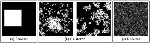
The four spatial configurations are examples among many potential landscape configurations between the spatial extreme of perfect concentration (‘compactness’) (Figure 1(a)) and perfect dispersion (Figure 1(c)). The perfect compact pattern consists of one single patch, whereas the perfect dispersed pattern is characterized by a maximum number of patches that depends on the perfect spatial partition of both thematic classes. For these extremes, the classification may be clear; however, generally accepted definitions and clear classifications schemes for spatial patterns in the transition zone between those extremes do not exist. For the two examples visualized in Figure 1(b) even a visual evaluation towards a higher degree of spatial dispersion is a difficult task and may result in varying evaluations with respect to the observer.

2.2. Design of the dispersion model for two-dimensional patterns

The focus of our investigation is the ‘settlement area’. We use the largest patch versus all other urban patches as a proxy to evaluate whether this largest patch is dominating an urban landscape or not. This proxy is related to monocentric city models, i.e. the basic idea that a dense core city is surrounded by a less dense surrounding area (e.g. Anas and Kim 1996). In its idealized form, the abstract representation of this urban landscape in a two-dimensional form is one large single patch (LP) reflecting the most compact urban pattern (Figure 1(a)). Any increase in the number of patches (NP) around this dominating largest patch turns the landscape into a more fragmented, less compact and thus more dispersed pattern. As a consequence, we use the number of patches as the second metric to evaluate the degree of compactness/dispersion of the landscape.

Using the previously introduced metrics LP and NP, we construct a two-dimensional model allowing a ranking of any possible pattern between compactness and dispersion (Figure 2). The mathematical details for the NP and LP are presented in Equations (1) and (2), where n_i is the number of patches of patch type (class) i in the landscape and a_i is the size of the area of patch j (class i) in pixels (McGarigal and Marks 1995; McGarigal, Cushman, and Ene 2012).(1) $\text{NP}=n_i\left(\text{absolute}\right),$(1) (2) $\text{LP}=\frac{\underset{i=1}{\stackrel{n}{max}}{a}_i}{{\sum }_{j=1}^n{a}_{ij}}\cdot 100(\text{relative},\text{percent}).$(2)

Figure 2. Schematic illustration of the model design for ranking binary patterns with respect to their spatial dispersion. Each arbitrary binary and two-dimensional pattern can be unambiguously located within the feature space of the model, which is defined only by two parameters, the NP on the x-axis and the LP on the y-axis.

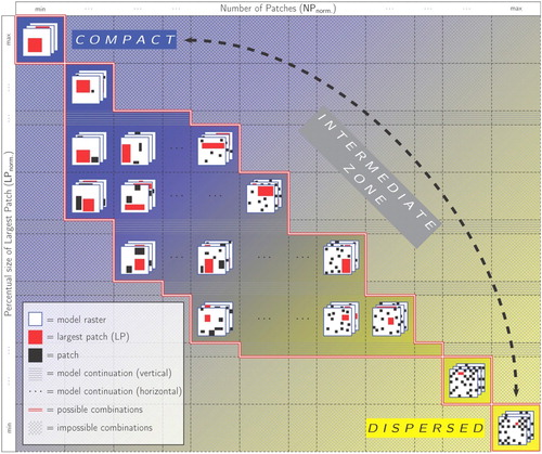
These two landscape features (LP, NP) span a two-dimensional space allowing a ranking of any pattern. In the remainder of this article, we refer to the feature space as ‘spatial dispersion’, as it is a function of the NP and the LP:$\text{Spatial dispersion }=f\left(\text{NP},\text{LP}\right).$

The model spanned by both parameters rank patterns with maximum values for the LP (100%) in the upper-left corner (Figure 2; perfectly compact). In contrast, if the LP is minimal and the complete class area (${\sum }_{j=1}^n{a}_{ij}$) is represented by the maximum possible number of non-coalescent individual patches, then the pattern is ranked in the lower-right corner (Figure 2; perfectly dispersed). All possible pattern configurations between the defined, perfectly compact and the perfectly dispersed patterns are in the intermediate zone of the feature space. The schematic illustration of the dispersion model in Figure 2 demonstrates that all parameter combinations of the NP and LP are clearly located within the model.

We scale the model to equal-ranges for the NP as well as the LP by normalizing the values (varying from 0 to 100 for NP_n on the x-axis and for LP_n on the y-axis). The mathematical details for normalizing NP_n and LP_n are presented in Equations (3) and (4).(3) $\text{N}{\text{P}}_n=\frac{\text{NP}-1}{({\sum }_{j=1}^n{a}_{ij})-1}\cdot 100,0\text{\%}\le \text{N}{\text{P}}_n\le 100\text{\%},$(3) (4) $\text{L}{\text{P}}_n=\frac{\text{LP}-{\displaystyle \frac{1}{{\sum }_{j=1}^n{a}_{ij}}}}{100-{\displaystyle \frac{1}{{\sum }_{j=1}^n{a}_{ij}}}}\cdot 100,0\text{\%}\le \text{L}{\text{P}}_n\le 100\text{\%}.$(4)

Every landscape pattern can be located within the feature space. We derive a single metric for classification, the dispersion index (DI). To do so, we use the combination of the two parameters presented before, namely, NP_n and LP_n. Both parameters are weighted equally (see Equations (3)–(5)).(5) $\text{DI}=\frac{\text{N}{\text{P}}_n+(100-\text{L}{\text{P}}_n)}{2}\left(\text{unit - less}\right).$(5)

3. Application of the DI: ranking of artificial spatial patterns

For testing the DI, we create artificial patterns. We do so because the detection of any theoretically possible spatial configuration is challenging, as the possible amount of different spatial patterns rises to a higher power if we vary the share of class area or the spatial extents. Thus, for testing the model-based conceptualization of landscape patterns, we introduce two model restrictions in this experiment:

1. We limit the spatial extent of the respective landscape for the model to a fixed square with a constant dimension and therefore with a constant landscape area (A = const.), even if borders of the particular landscape seemed artificial.

2. We fix the number of class areas as well as the share of class area. In our model, only two classes were considered: settlement and non-settlement.

Both model prerequisites result in a significant reduction in possible cases. In this first approach to the model, we consider only patterns for which Equations (6) and (7) are true.(6) $\frac{100-\text{L}{\text{P}}_n}{\text{N}{\text{P}}_n}\le 1,$(6) (7) $\text{L}{\text{P}}_n\le 100-\text{N}{\text{P}}_n.$(7)

These model prerequisites in Equations (6) and (7) explain that mathematically impossible parameter combinations exist as the value of NP_n determines the parameter LP_n and vice versa. For example, a high relative LP_n does not allow for a high NP_n at the same time. These impossible parameter combinations are shown in the lower-left and upper-right corners of Figure 2.

For our experimental set-up, we produce artificial patterns for each combination of NP and LP (DI values between 0 and 100) in a controlled way (see Appendix 1 in supplementary information for the methodological details of pattern generation). For each individual combination, we permutate 10 random versions to account for the variability of patterns, even with equal DI values. This approach results in more than 300,000 artificial patterns for testing.

We test the meaning and interpretation of the DI values illustrating the selected samples: If the DI approaches 0, then the pattern is compact with a low number of patches, which is a pattern that could be interpreted as spatially compact and a dominating core city (patterns 1–3 in Figure 3, with DI values smaller than 20, representing different spatial configurations of this type). In contrast, if the DI approaches 100, then the number of patches is high, whereas the dominance of the largest patch is low; as a consequence, a spatially dispersed landscape (patterns 7–9 in Figure 3 with DI values greater than 65) is represented. All examples between the ranges (patterns 4–6) represent different configurations of complex, clustered spatial forms. While the terminological descriptions of the varying types and the visual interpretations leave space for subjectivity, the DI allows unambiguous ranking.

Figure 3. Examples for artificial patterns and the corresponding values for the NP, NP_n, LP, LP_n and DI. White pixels = class ‘1’, red Pixels (in print darker pixels) = largest patch of class ‘1’, and black pixels = background. NP = absolute number of patches; LP = percent area of the largest patch; NP_n = normalized number of patches (relative); LP_n = normalized percent area of the largest patch (relative).

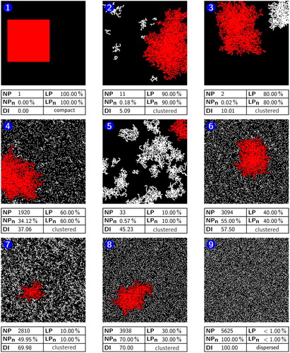
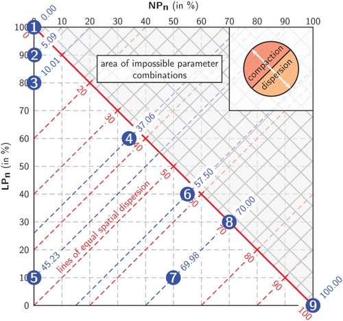
When we transfer these selected sample patterns into the developed model, an unambiguous classification of each individual pattern within the two-dimensional feature space with respect to dispersion is possible (Figure 4). The perfect representation of a compact, monocentric pattern (1) is classified in the upper-left corner (DI = 0). The perfect representation of a dispersed pattern (9) is in the lower-right corner (DI = 100). The remaining patterns (2)–(8) can be compared relative to each other by the DI and in absolute terms in relation to the perfect pattern representations. It is interesting to note that the two patterns (7) and (8) almost feature the same DI value of 70; the location in the model describes their pattern differences, with (8) being slightly more dispersed, as the significantly higher relative number of patches (for (8) 70% vs. 50% for (7)) overcomes the significantly lower relative largest patch dominance (for (8) 30% vs. 10% for (7)).

Figure 4. Two-dimensional feature space spanned by the parameters NP_n and LP_n. The numbered points symbolize the locations within the model of the related patterns displayed in Figure 3. The ‘area of impossible parameter combinations’ is because the value of the NP_n determines the corresponding parameter LP_n and vice versa.

4. Validity of other spatial metrics within the design of the dispersion model

The developed dispersion model relies on two parameters – NP_n and LP_n – for a quantitative description of artificially generated patterns. With it, we have shown that spatial patterns can be unambiguously measured with respect to dispersion. However, manifold other metrics have been developed for describing patterns using different perspectives, i.e. metrics are, for example, relating to the form of patches or to distances between patches. Many studies apply these metrics and develop assumptions, e.g. related to the evaluation of the degree of dispersion of patterns. However, it remains unclear whether these metrics allow an unambiguous interpretation in general and within the developed model design in particular. In the following, we test selected spatial metrics which have been commonly applied in other studies whether they allow an unambiguous interpretation.

For the test, we select spatial metrics and apply them onto the 300,000 artificially generated patterns: We select the Patch Area (AREA) from the ‘area and edge metrics’. The constant share of the class areas in the artificially generated patterns leads to an indirect proportional relation between number of patches (NP) and area of the largest patch (LP). Thus, we expect a decreasing mean patch area during a rising grade of spatial dispersion. From the category shape metrics, we selected the Shape Index (SHAPE) as one metric which is based on the perimeter–area relationship. The shape index measures the patch shape or the normalized ratio of patch perimeter to area in which the complexity of patch shape is compared to a standard shape (square) of the same size. The shape index approaches 1 if the shape of the investigated patch is a single square or maximally compact patch of the corresponding type, and increases infinitely as the patch becomes more disaggregated (Lv, Dai, and Sun 2012). Beyond, we test the Fractal Dimension Index (FRAC), another normalized shape index based on perimeter–area relationships in which the perimeter and area are log-transformed. FRAC indicates departures from Euclidean geometries and measures increasing shape complexity. We furthermore select the Contiguity Index (CONTIG). It assesses patch shape based on the spatial connectedness or contiguity of cells within a patch. This index quantifies the spatial contiguity of all patches. In consequence, lower metric values are expected for dispersed patterns. The Related Circumscribing Square Index (SQUARE) evaluates the shape of patches and is based on the ratio of patch area to the area of the smallest circumscribing square. The related circumscribing square provides a measure of overall patch elongation. This index may be particularly useful for distinguishing patches that are both linear (narrow) and elongated. Within the group of the aggregation metrics, we calculate the Euclidean Nearest Neighbor (ENN) Distance. It calculates the shortest straight-line distance between a focal patch and its nearest patch neighbor of the same class. We expect that rising dispersion with rising NP_n and decreasing LP_n goes along with a decreasing index value for the ENN Distance. We apply the Landscape Shape Index (LSI). It is a normalized ratio of the patch perimeters to the class area in which the total length of edge is compared to a landscape with a standard shape (square) of the same size and without any internal edge; values greater than one indicate increasing levels of internal edge and corresponding decreasing aggregation of patch types. Similar to the LSI the Normalized Landscape Shape Index (nLSI) is the normalized version of LSI that scales the metric to range 0–1 between the theoretical minimum and maximum index values; values approaching one indicate increasing levels of internal edge and corresponding decreasing aggregation of patch types. All mathematical details are presented in detail in Appendix 2 (supplementary information).

In the following, we evaluate whether these spatial metrics can be used in the context of our proposed model within an unambiguous interpretation regarding the measured settlement pattern dispersion. As the DI ranks all patterns, we assume spatial metrics allow meaningful interpretations when medians of spatial metrics applied to the artificially generated raster data with defined parameter combinations regarding NP_n and LP_n exhibit a mathematical monotonic trend in two cases: (1) The behavior of the values must be monotonic rising (or decreasing) during a rising NP_n when LP_n is constant. (2) At the same time, the behavior of values must be monotonic rising (or decreasing) during a decreasing LP_n when NP_n is constant. For validation, we calculate four statistical parameters per metric: Arithmetic mean, area-weighted mean, standard deviation and coefficient of variation to identify whether trends to higher dispersion or higher compaction can be measured or not.

Figure 5 visualizes the example of the LSI. In this case, artificial rasters are applied where the LP_n is kept constant with 20% and a rising NP_n can be tested, i.e. we consider patterns with an increasing grade of dispersion. And, in addition, we keep NP_n constant with 8.87% and test a rising LP_n indicating a decreasing grade of dispersion. We perform this analysis systematically for all selected spatial metrics with alternating fixed LP_n as well as NP_n and permutation of the particular other metric.

Figure 5. Behavior of the Landscape Shape Index (LSI) for (a) an increasing grade of dispersion caused by rising NP_n and constant LP_n of 20% and (b) for a decreasing grade of dispersion caused by rising LP_n and constant NP_n of 8.87% (500 patches).

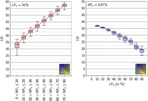
Figure 5(a) shows a direct positive relationship between NP_n of the analyzed artificial rasters and the measured LSI values. In addition, Figure 5(b) reveals a negative relationship between LP_n and the values for LSI. The combination of an increasing monotony in case of NP_n with a decreasing monotony in the case of LP_n allows to conclude that the LSI is a fully qualified index to substantiate shifts regarding grades of spatial dispersion according to the above-mentioned hypothesis. In contrast, most other tested metrics do not corroborate the mentioned hypothesis because a monotonic and thus an unambiguous behavior is not measured.

Table 1 presents all 26 analyzed metrics with respect to their interpretability concerning spatial dispersion. Although most of the indices do not show the above-explained monotonic relationship between NP_n and LP_n, at least six of the 26 metrics are found to allow an unambiguous interpretation regarding spatial dispersion.

Table 1. 26 selected class-level metrics and their behavior regarding monotony in horizontal respectively vertical direction within the model.

Note: d = monotonically decreasing; r = monotonically rising, 0 = no metric calculated; - = no monotony; lines without a dash = parameter which is suited for interpretation regarding spatial dispersion; lines with a dash = parameter which is not suited for interpretation regarding spatial dispersion; line with only one dash = parameter which is partly suited for interpretation regarding spatial dispersion.

5. Influence of model parameter variations

The chosen areas of interest as well as the spatial resolutions of the input data influence spatial metrics. For an assessment of the validity of the model conceptualization, we systematically test the sensitivity of these two factors onto the DI: On the one hand, we test the influence of the extent. Therefore, we systematically enlarge the extent around a city center from 20 km to 100 km by 10 km steps. With the smallest extent, we assume the main core of a city is covered. With rising extents, the hinterlands and rural surroundings get covered in addition. In turn, we expect the DI to increase with rising extents. On the other hand, we systematically test the influence of spatial resolutions of the input data. We test the spatial resolution representing settlement patterns starting with the Landsat resolution of 30 m. For the test, we decrease the resolution to 50, 200, 500 and 1000 m. With lower resolutions, we expect the patterns to become more dispersed. For the test, we select a sample settlement pattern from the area of Warzaw, Poland. Warzaw is a large city surrounded by a less urbanized area. Figure 6 illustrates the variations tested with respect to extent and spatial resolution.

Figure 6. Influence of the spatial extent and spatial resolutions onto the dispersion index.

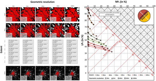
Figure 6 clearly demonstrates the influence of extent and spatial resolution onto the DI. We find the pattern of Warzaw with a 20-km extent obviously highly compact. The DI values range from 1.4 at 30 m resolution to 8.4 at 1000 m. With increasing extents, the DI values increase systematically. At 100 km extents, we find DI values from 29.4 at 30 m resolution to 51.7 at 1000 m resolution.

We find that as long as the input data characteristics are hold constant, the relative ranking in the DI remains constant. These results are confirming findings, e.g. by Lechner et al. (2013). However, the absolute evaluation of the landscape dispersion varies. In consequence, the model design is considered appropriate for comparing settlement patterns at the same spatial extent and the same spatial resolution. Another legitimate option is when approaches are developed finding extents in different areas of interest which are conceptually considered comparable.

6. Application of the DI: ranking of real-world patterns

In the following sections, we apply the introduced model and the related DI to urban land cover classifications of the selected areas. For this purpose, classifications of settlement areas are based on EO data for the time steps 1975, 1990, 2000 and 2010 (for methodological details on the classification procedure, the definition of the class and the related accuracies, we refer to Taubenböck et al. 2012 and Klotz et al. 2016).

We aim to test the development of the DI over time and compare city patterns across space. To do so, we select five different sample cities with varying socioeconomic dynamics over the 35 years of monitoring and differing pattern configurations: We apply the model to two dynamically growing urban regions in China – Shenzhen and Dongguan – both located in the mega-region Hong Kong-Shenzhen-Guangzhou. In contrast, we apply the model to two urban regions in Germany – Cologne and Frankfurt am Main – that have not experienced dynamic changes since the 1970s. Finally, we apply the model to a city where we assume that dynamics changed over time: Warsaw, Poland. For reasons of comparability, we use a fixed spatial entity of 30 × 30 km around the respective city centers.

The urban land cover patterns and their temporal evolution in the five sample cities are visualized in Figure 7. In addition to the classified physical expansion of urban areas over 35 years, the largest patch is highlighted (in red). In general, it is clear that the ongoing process of urbanization physically manifests itself in the emergence of more complex, irregular spatial patterns. The once clear core–periphery divide in the Chinese cities has diminished in favor of a spatially extended, scattered urban field without a visible urban core. In contrast, the German cities were already large in the 1970s, and their patterns are relatively stable over time. However, this figure also illustrates that an evaluation of the compactness or dispersion of a pattern is not obvious; e.g. comparing the patterns of Cologne and Frankfurt for the year 2000 does not demonstrate a clear visual interpretation regarding spatial dispersion.

Figure 7. Binary settlement patterns for the cities Shenzhen and Dongguan in China, Frankfurt am Main and Cologne in Germany and Warsaw in Poland at four different time steps (1975, 1990, 2000, 2010). Areas that are covered by settlement elements are displayed in white. The largest urban patch (LP) is visualized in grey. The dimension of each frame is 30 × 30 kilometers around a defined city center; the geometric resolution of each raster is 200 meters.

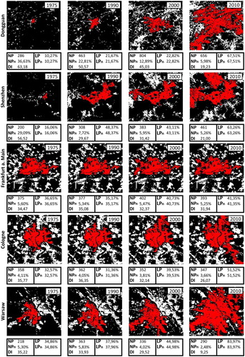
An unambiguous evaluation of the compactness/dispersion of a pattern is visually challenging. The classification of the degree of dispersion allows the allocation of all 20 individual patterns displayed in Figure 7 to a unique position within the designed dispersion model. The resulting DI values for each raster are displayed in Figure 7, whereas the unique positions of all 20 patterns within the feature space are illustrated in Figure 8.

Figure 8. Shifts in dispersion for the five sample cities within the two-dimensional feature space spanned by the parameters NP_n and LP_n.

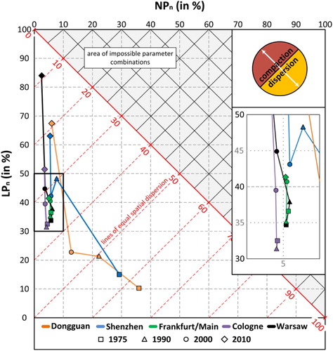
In general, we find that physical urban expansion leads in all five examples towards a more compact spatial pattern over the 35 years of monitoring. However, the degree of dispersion and the spatial dynamics vary significantly: The most dynamic change of patterns occurred in the Chinese regions. The example of Dongguan shows the transition of a small city with a small largest patch and a disperse, agricultural settlement pattern in 1975 (DI value of 63.18) to a very large and compact agglomeration dominated by a very large patch in 2010 (DI of 19.23). One can interpret the spatial growth characteristic of Dongguan as follows: Between 1975 and 2010, the largest patch grew at a very high rate. In parallel, the normalized number of patches was constantly decreasing due to the coalescence of once separate patches, although the absolute number of patches was increasing. Essentially, the same development is measured for Shenzhen.

In contrast, the urban regions of Cologne and Frankfurt am Main feature a basically constant DI (e.g. Frankfurt in 1975 with DI of 34.47 was 31.94 in 2010). The expansion of both cities was marginal. The most significant change occurred for Cologne as re-densification processes led to coalescence of the core city (largest patch) with the surrounding large patches. This, as a consequence, led to an increase of the largest patch index and an increase in the compactness of the pattern. In Frankfurt am Main, the largest patch did not experience any coalescence with the surrounding urban patches over the monitoring period. This could be interpreted as the spatial manifestation of a greenbelt policy that has shaped Frankfurt’s urban development for decades.

The city of Warsaw, although it experienced a dynamic expansion of its urbanized area, measured only slight changes towards compaction from 1975 until 2000. However, from 2000 to 2010, re-densification processes in the city center led to coalescence of the two defining largest patches. This led to a significant compaction of the urban landscape pattern, and it is worth mentioning that Warsaw had the lowest DI of all five case study regions in 2010.

The implementation of spatial patterns and their evolution over time for five sample cities into our model enable – next to a relative comparison among them – an evaluation of dispersion and compactness trends within a theoretical spectrum of urban landscape configurations. The presented results seem to confirm the claim discussed in the introduction, according to which long-lasting urbanization forces create compact urban patterns at higher (‘mega-urban’) spatial scales. Following this line of thought, a dispersed, ‘sprawling’ urban landscape is an intermediate state alongside a long-term transition from a pre-industrial, rural landscape with smaller cities and more or less evenly distributed agricultural settlements (higher DI values would be expected) into a spatially extended, continuously urbanized regional territory (with lower DI values).

In relation to the artificially generated patterns, we observe for our sample that real-world patterns of cities typically feature DI values below 50 or mostly below 40 (16 out of 20 patterns have DI values below 40). The few examples with DI values larger than 50 relate to Chinese cities and their patterns measured in the 1970s or the 1990s. These values refer to pre-urban and pre-industrial environments with typically many small patches without dominating large core areas (cf. Figure 7). Dongguan, as an example of real-world patterns, featured a DI of 63.18 in 1975. The spatial pattern shows a typical rural, scattered settlement pattern with the largest patch not dominating the area.

7. Discussion and concluding remarks

The characterization and understanding of (urban) spatial patterns are of central concern in the spatial sciences (Klippel, Hardisty, and Li 2011). As every single spatial pattern configuration is unique across the globe and no two of these spatial configurations are likely to be identical, it is crucial to provide methods to systematically measure convergent and divergent development trends. However, the unambiguous evaluation of spatial patterns with respect to compactness/dispersion is challenging. Thus, the primary goal of this work is to suggest a conceptualization of spatial dispersion for two-dimensional (settlement) patterns. With the introduced model, the classification of any two-dimensional binary raster with respect to the degree of (urban) dispersion becomes feasible.

In our approach, we reduced the model complexity to the physical perspective of two-dimensional spatial patterns. This, of course, is a simplification of the urban environment that was necessary to understand patterns in a holistic sense. Important dimensions of urban spatial patterns such as the intensity of urban land uses (population density and employment density, among others) or issues of functional centrality and concentration are not considered. However, the systematic measurement and consistent comparison of generalized spatial patterns allow insights into urbanization trajectories. These approaches become increasingly relevant as the availability of global settlement classifications from EO data at a high resolution increases. We are aware that real-world input data might suffer from classification errors and that these can cause consequential mistakes in measuring patterns. Kleindl, Powell, and Hauer (2015) reveal that each metric has a different sensitivity to error. This is especially true when patches close to each other are measured as spatially connected (or not), which can significantly influence the dimension of the largest patch. However, recent studies show that the latest remote sensing settlement classifications produce accuracy rates far beyond 85% for urbanized regions (e.g. Klotz et al. 2016). This allows us to assume that the measured trends of dispersion are correct. The selection of the area of interest is another important issue. While the model is independent from the chosen area of interest, the question arises as to whether it is meaningful to compare two cities with varying spatial patterns/sizes/forms based on a fixed area of interest (in our case, we chose 30 × 30 km). From a spatial and mathematical point of view, comparing two cities in this way is correct and acceptable, but to determine if it is meaningful from a geographical point of view, they must be tested by further applications with varying test sites and areas of interests.

Our model aims at providing a better understanding of spatial complexities in today’s urban environments. The systematic application of the model on urban land cover patterns across the globe offers a new analytic perspective on global spatial urbanization processes and provides a methodological basis for categorizing urban areas into classes of different spatial pattern characteristics and development trends. Such information is highly valuable for understanding and predicting urban growth as well as for evaluating development patterns and their positive and negative externalities with respect to the needs of urban planning and resource conservation. In this case, the results confirm the claim that long-term urbanization forces create compact urban patterns at higher (‘mega-urban’) spatial scales and that a dispersed, ‘sprawling’ urban landscape is an intermediate state. This result, of course, needs to be confirmed by a significantly larger sample of cities.

Furthermore, our model contributes to the ongoing discussion of general, widespread trends in urbanization and urban growth and/or the uniqueness of cities and urban spaces (see, for example, Robinson 2016 and Scott and Storper 2015). In the second decade of the twenty-first century, we have entered an era where geodata and geoinformation are available at an unprecedented scope and spatial resolution. However, research is not keeping pace in terms of developing concepts and techniques that add value to these immense sets of geodata. The quantitative measurement of spatial patterns is such an example, where an unambiguous measurement and, as a consequence, a clear interpretation are still challenging. This paper’s model-based approach aims to provide a conceptual idea for a systematic and comparative evaluation of (urban) patterns with respect to issues of structure and form. Especially in times where urbanization is transforming global society and, with it, the built landscapes across the world, robust techniques and indicators need to be systematically developed and applied for a better empirical understanding of processes related to these spatial landscape changes.

Acknowledgements

We sincerely thank Michael Wiesner for his dedication to this work.

Disclosure statement

No potential conflict of interest was reported by the authors.

ORCID

Hannes Taubenböck http://orcid.org/0000-0003-4360-9126

Michael Wurm http://orcid.org/0000-0001-5967-1894

References

- Anas, A., R. Arnott, and K. Small. 1998. “Urban Spatial Structure.” Journal of Economic Literature 36 (3): 1426–1464.
- Anas, A., and I. Kim. 1996. “General Equilibrium Models of Polycentric Urban Land Use with Endogenous Congestion and Job Agglomeration.” Journal of Urban Economics 40 (2): 232–256. doi:10.1006/juec.1996.0031.
- Angel, S. 2012. Planet of Cities. Cambridge, MA: Lincoln Institute of Land Policy.
- Angel, S., and A. Blei. 2016. “The Spatial Structure of American Cities: The Great Majority of Workplaces Are No Longer in CBDs, Employment sub-Centers or Live-Work Communities.” Cities (London, England) 51: 21–35.
- Angel, S., J. Parent, D. L. Civco, A. M. Blei, and D. Potere. 2011. “The Dimensions of Global Urban Expansion: Estimates and Projections for All Countries, 2000-2050.” Progress in Planning, 75 (2): 53–107.
- Antrop, M. 2004. “Landscape Change and the Urbanization Process in Europe.” Landscape and Urban Planning 67: 9–26.
- Batty, M. 2008. “The Size, Scale, and Shape of Cities.” Science 319: 769–771.
- Batty, M., E. Besussi, K. Maat, and J. J. Harts. 2004. “Representing Multifunctional Cities: Density and Diversity in Space and Time.” Built Environment 30 (4): 324–337. doi:10.2148/benv.30.4.324.57156.
- Bender, D. J., L. Tischendorf, and L. Fahrig. 2003. “Using Patch Isolation Metrics to Predict Animal Movement in Binary Landscapes.” Landscape Ecology 18 (1): 17–39.
- Brownstone, D., and T. F. Golob. 2009. “The Impact of Residential Density on Vehicle Usage and Energy Consumption.” Journal of Urban Economics 65: 91–98.
- Burchell, R. W., A. Downs, B. McCann, and S. Mukherji. 2005. Sprawl Costs: Economic Impacts of Unchecked Development. Washington: Island Press.
- Burchell, R. W., and S. Mukherji. 2003. “Conventional Development Versus Managed Growth: The Costs of Sprawl.” American Journal of Public Health 93 (9): 1534–1540.
- Burger, M., and E. Meijers. 2012. “Form Follows Function? Linking Morphological and Functional Polycentricity.” Urban Studies 49 (5): 1127–1149.
- Cieslewicz, D. J. 2002. “The Environmental Impacts of Sprawl.” In Urban Sprawl. Causes, Consequences & Policy Responses, edited by G. D. Squires, 23–38. Washington, DC: The Urban Institute Press.
- Esch, T., M. Marconcini, D. Marmanis, J. Zeidler, S. Elsayed, A. Metz, A. Müller, and S. Dech. 2014. “Dimensioning Urbanization – An Advanced Procedure for Characterizing Human Settlement Properties and Patterns Using Spatial Network Analysis.” Applied Geography 55: 212–228.
- Esch, T., H. Taubenböck, A. Roth, W. Heldens, A. Felbier, M. Thiel, M. Schmidt, M. Müller, A. Müller, and S. Dech. 2012. “TanDEM-X Mission: New Perspectives for the Inventory and Monitoring of Global Settlement Patterns.” Journal of Selected Topics of Applied Earth Observation 6: 061702.
- EEA / FOEN (European Environment Agency and Swiss Federal Office for the Environment). 2016. Urban Sprawl in Europe. Joint EEA-FOEN report No. 11/2016. Luxemburg, European Environment Agency and Federal Office for the Environment.
- Ewing, R., and S. Hamidi. 2015. “Compactness Versus Sprawl: A Review of Recent Evidence from the United States.” City & Metropolitan Planning 30 (4): 413–432.
- Ewing, R., and F. Rong. 2008. “The Impact of Urban Form on U.S. Residential Energy use.” Housing Policy Debate 19 (1): 1–30.
- Florida, R., T. Gulden, and C. Mellander. 2008. “The Rise of the Mega-Region.” Cambridge Journal of Regions, Economy and Society 1 (3): 459–476.
- Fragkias, M., and K. Seto. 2009. “Evolving Rank-Size Distributions of Intra-Metropolitan Urban Clusters in South China.” Computers, Environment and Urban Systems 33 (3): 189–199.
- Galster, G., R. Hanson, M. R. Ratcliffe, H. Wolmann, S. Coleman, and J. Freihage. 2001. “Wrestling Sprawl to the Ground: Defining and Measuring an Elusive Concept.” Housing Policy Debate 12: 681–717.
- Garcia-López, MÀ, and I. Muñiz. 2010. “Employment Decentralisation: Polycentricity or Scatteration? The Case of Barcelona.” Urban Studies 47 (14): 3035–3056.
- Herold, M., N. C. Goldstein, and K. C. Clarke. 2003. “The Spatiotemporal Form of Urban Growth: Measurement, Analysis and Modeling.” Remote Sensing of Environment 86: 286–302.
- Hortas-Rico, M., and A. Solé-Ollé. 2010. “Does Urban Sprawl Increase the Costs of Providing Local Public Services? Evidence From Spanish Municipalities.” Urban Studies 47 (7): 1513–1540.
- Huang, J., X. X. Lu, and J. M. Sellers. 2007. “A Global Comparative Analysis of Urban Form: Applying Spatial Metrics and Remote Sensing.” Landscape and Urban Planning 82: 184–197.
- Jabareen, Y. R. 2006. “Sustainable Urban Forms: Their Typologies, Models and Concepts.” Journal of Planning Education and Research 26 (1): 38–52.
- Jaeger, J., and C. Schwick. 2014. “Improving the Measurement of Urban Sprawl: Weighted Urban Proliferation (WUP) and its Application to Switzerland.” Ecological Indicators 38: 294–308.
- Johnson, M. P. 2001. “Environmental Impacts of Urban Sprawl: a Survey of the Literature and Proposed Research Agenda.” Environment and Planning A 33 (4): 717–735.
- Kleindl, W., S. Powell, and F. Hauer. 2015. “Effect of Thematic Map Misclassification on Landscape Multi-Metric Assessment.” Environmental Monitoring and Assessment 187 (6): 257.
- Klippel, A., F. Hardisty, and R. Li. 2011. “Interpreting Spatial Patterns: An Inquiry into Formal and Cognitive Aspects of Tobler’s First Law of Geography.” Annals of the Association of American Geographers, 101 (5): 1011–1031.
- Klotz M., T. Kemper, C. Geiß, T. Esch, and H. Taubenböck. (2016). “How Good is the Map? A Multi-Scale Cross-Comparison Framework for Global Settlement Layers: Evidence from Central Europe.” Remote Sensing of Environment, 178: 191–212.
- Knaap, G.-J., Y. Song, R. Ewing, and K. Clifton. 2005. “ Seeing the Elephant: Multi-Disciplinary Measures of Urban Sprawl.” Urban Studies and Planning Program, University of Maryland. http://smartgrowth.umd.edu/assets/documents/research/knaapsongewingetal_2005.pdf.
- Kraas, F., G. Mertins, et al. 2014. “Megacities and Global Change.” In Megacities. Our Global Urban Future, edited by F. Kraas, 1–8. Heidelberg: Springer.
- Lang, S., and T. Blaschke. 2007. Landschaftsanalyse mit GIS. 20 Tabellen. Stuttgart: Ulmer.
- Lang, R., and P. K. Knox. 2009. “The New Metropolis: Rethinking Megalopolis.” Regional Studies 43 (9): 789–802.
- Lechner, A. M., K. J. Reinke, Y. Wang, and L. Bastien. 2013. “Interactions Between Landcover Pattern and Geospatial Processing Methods: Effects on Landscape Metrics and Classification Accuracy.” Ecological Complexity 15: 71–82.
- LSE Cities. 2014. Cities and Energy: Urban Morphology and Heat Energy Demand. London: LSE Cities, London School of Economics and Political Science.
- Luck, M., and J. Wu. 2002. “A Gradient Analysis of Urban Landscape Pattern: A Case Study from the Phoenix Metropolitan Region, Arizona, USA.” Landscape Ecology 17 (4): 327–339.
- Lv, Z.-q., F.-q. Dai, and C. Sun. 2012. “Evaluation of Urban Sprawl and Urban Landscape Pattern in a Rapidly Developing Region.” Environmental Monitoring and Assessment 184 (10): 6437–6448.
- McGarigal, K., S. A. Cushman, and E. Ene. 2012. FRAGSTATS v4: Spatial Pattern Analysis Program for Categorical and Continuous Maps. Computer software program produced by the authors at the University of Massachusetts, Amherst.
- McGarigal, K., and B. Marks. 1995. FRAGSTATS. Spatial Pattern Analysis Program for Quantifying Landscape Structure. Portland, OR: U.S. Dept. of Agriculture Forest Service Pacific Northwest Research Station.
- Mubareka, S., E. Koomen, C. Estreguil, and C. Lavalle. 2011. “Development of a Composite Index of Urban Compactness for Land Use Modelling Applications.” Landscape and Urban Planning. doi:10.1016/j.landurbplan.2011.08.012.
- Newman, P., and J. R. Kenworthy. 2006. “Urban Design to Reduce Automobile Dependence.” Opolis 2 (1): 35–52.
- OECD. 2010. Cities and Climate Change. Paris: OECD.
- OECD. 2012. Compact City Policies. A Comparative Assessment. Paris: OECD.
- Peiser, R. 1989. “Density and Urban Sprawl.” Land Economics 65 (3): 193–204.
- Peiser, R. 2001. “Decomposing Urban Sprawl.” Town Planning Review 72: 275–298.
- Pesaresi, M., G. Huadong, X. Blaes, D. Ehrlich, S. Ferri, L. Gueguen, and L. Zanchetta. 2013. “A Global Human Settlement Layer from Optical HR/VHR RS Data: Concept and First Results.” IEEE Journal of Selected Topics in Applied Earth Observations and Remote Sensing 6 (6): 2102–2131. doi:10.1109/JSTARS.2013.2271445.
- Poelmans, L., and A. Van Rompaey. 2009. “Detecting and Modelling Spatial Patterns of Urban Sprawl in Highly Fragmented Areas: A Case Study in the Flanders–Brussels Region.” Landscape and Urban Planning 93 (1): 10–19.
- Riitters, K. H., R. V. O’Neill, C. T. Hunsaker, J. D. Wickham, D. H. Yankee, S. P. Timmins, K. B. Jones, and B. L. Jackson. 1995. “A Factor Analysis of Landscape Pattern and Structure Metrics.” Landscape Ecology 10: 23–39.
- Robinson, J. 2016. “Comparative Urbanism: New Geographies and Cultures of Theorizing the Urban.” International Journal of Urban and Regional Research 40 (1): 187–199.
- Schneider, A., C. Chang, and K. Paulsen. 2015. “The Changing Spatial Form of Cities in Western China.” Landscape and Urban Planning 135 (March): 40–61.
- Schneider, A., and C. Woodcock. 2008. “Compact, Dispersed, Fragmented, Extensive? A Comparison of Urban Growth in Twenty-Five Global Cities Using Remotely Sensed Data, Pattern Metrics and Census Information.” Urban Studies 45: 659–692.
- Schumaker, N. H. 1996. “Using Landscape Indices to Predict Habitat Connectivity.” ECOLOGY 77 (4): 1210–1225.
- Scott, A. J., and M. Storper. 2015. “The Nature of Cities: the Scope and Limits of Urban Theory.” International Journal of Urban and Regional Research 39 (1): 1–15.
- Seto, K. C., and M. Fragkias. 2005. “Quantifying Spatiotemporal Patterns of Urban Land-Use Change in Four Cities of China with Time Series Landscape Metrics.” Landscape Ecology 20 (7): 871–888.
- Siedentop, S. 2005. “Urban Sprawl - verstehen, messen, steuern.” DISP 160: 23–35.
- Siedentop, S. 2015. “Ursachen, Ausprägungen und Wirkungen der globalen Urbanisierung – ein Überblick.” In Globale Urbanisierung – Perspektive aus dem All, edited by H. Taubenböck, M. Wurm, T. Esch, and S. Dech, 11–21. Berlin: SpringerSpektrum.
- Siedentop, S., and S. Fina. 2010. “Monitoring Urban Sprawl in Germany: Towards a GIS-Based Measurement and Assessment Approach.” Journal of Land Use Science 5 (2): 73–104.
- Siedentop, S., and S. Fina. 2012. “Who Sprawls Most? Exploring the Patterns of Urban Growth Across 26 European Countries.” Environment and Planning A: Economy and Space 44 (11): 2765–2784.
- Silva, M., V. Oliveira, and V. Leal. 2017. “Urban Form and Energy Demand: A Review of Energy-Relevant Urban Attributes.” Journal of Planning Literature 32 (4): 346–365.
- Speir, C., and K. Stephenson. 2002. “Does Sprawl Cost us all? Isolating the Effects of Housing Patterns on Public Water and Sewer Costs.” Journal of the American Planning Association 68 (1): 56–70.
- SRU (Sachverständigenrat für Umweltfragen). 2016. Umweltgutachten 2016. Impulse für eine integrative Umweltpolitik. Wiesbaden: SRU.
- Stone Jr. B., A. C. Mednick , T. Holloway, and S. N. Spak. (2007). “Is Compact Growth Good for Air Quality?” Journal of the American Planning Association 73 (4): 404–418.
- Sudhira, H. S., T. V. Ramachandra, and K. S. Jagadish. 2004. “Urban Sprawl: Metrics, Dynamics and Modelling Using GIS.” International Journal of Applied Earth Observation and Geoinformation 5 (1): 29–39.
- Taubenböck, H., T. Esch, A. Felbier, M. Wiesner, A. Roth, and S. Dech. 2012. “Monitoring Urbanization in Mega Cities from Space.” Remote Sensing of Environment, 117, 162–176.
- Taubenböck, H., M. Klotz, M. Wurm, J. Schmieder, B. Wagner, M. Wooster, and T. Esch. 2013. “Delineation of Central Business Districts in Mega City Regions Using Remotely Sensed Data.” Remote Sensing of Environment 136: 386–401.
- Taubenböck, H., I. Standfuß, M. Wurm, A. Krehl, and S. Siedentop. 2017. “Measuring Morphological Polycentricity – A Comparative Analysis of Urban Mass Concentrations Using Remote Sensing Data.” Computers, Environment and Urban Systems 64: 42–56.
- Taubenböck, H., M. Wegmann, A. Roth, H. Mehl, and S. Dech. 2009. “Urbanization in India – Spatiotemporal Analysis Using Remote Sensing Data.” Computers, Environment and Urban Systems 33 (3): 179–188.
- Taubenböck, H., and M. Wiesner. 2015. “The Spatial Network of Megaregions – Types of Connectivity Between Cities Based on Settlement Patterns Derived from EO-Data.” Computers, Environment and Urban Systems 54: 165–180.
- Taubenböck, H., M. Wiesner, A. Felbier, M. Marconcini, T. Esch, and S. Dech. 2014. “New Dimensions of Urban Landscapes: The Spatio-Temporal Evolution from a Polynuclei Area to a Mega-Region Based on Remote Sensing Data.” Applied Geography 47: 137–153.
- Theobald, D. M., J. R. Miller, and N. Thompson Hobbs. 1997. “Estimating the Cumulative Effects of Development on Wildlife Habitat.” Landscape and Urban Planning 39: 25–36.
- Tsai, Y.-H. 2005. “Quantifying Urban Form: Compactness Versus ‘Sprawl’.” Urban Studies 42 (1): 141–161.
- United Nations. 2016. World Urbanization Prospects – The 2015 Revision. New York: United Nations Publication.
- United Nations Human Settlements Programme. (2009). Planning Sustainable Cities: Global Report on Human Settlements 2009. Nairobi, Kenya.
- Wurm, M., P. d’Angelo, P. Reinartz, and H. Taubenböck. 2014. “Investigating the Applicability of Cartosat-1 DEMs and Topographic Maps to Localize Large-Area Urban Mass Concentrations.” JSTARS 7 (11): 4138–4152.
- Zhang, L., J. Wu, Y. Zhen, and J. Shu. 2004. “RETRACTED: A GIS-Based Gradient Analysis of Urban Landscape Pattern of Shanghai Metropolitan Area, China.” Landscape and Urban Planning 69 (1): 1–16.