Object-based image analysis of suburban landscapes using Landsat-8 imagery

ABSTRACT

Many experiments of object-based image analysis have been conducted in remote sensing classification. However, they commonly used high-resolution imagery and rarely focused on suburban area. In this research, with the Landsat-8 imagery, classification of a suburban area via the object-based approach is achieved using four classifiers, including decision tree (DT), support vector machine (SVM), random trees (RT), and naive Bayes (NB). We performed feature selection at different sizes of segmentation scale and evaluated the effects of segmentation and tuning parameters within each classifier on classification accuracy. The results showed that the influence of shape on overall accuracy was greater than that of compactness, and a relatively low value of shape should be set with increasing scale size. For DT, the optimal maximum depth usually varied from 5 to 8. For SVM, the optimal gamma was less than or equal to 10⁻², and its optimal C was greater than or equal to 10². For RT, the optimal active variables was less than or equal to 4, and the optimal maximum tree number was greater than or equal to 30. Furthermore, although there was no statistically significant difference between some classification results produced using different classifiers, SVM has a slightly better performance.

KEYWORDS:

• Land cover
• remote sensing
• object-based
• classifier
• feature selection

1. Introduction

The classification of remote sensing imagery presents important significance for a number of applications, such as resources investigation (Ma et al. 2014), environmental assessment (Wu et al. 2014a), and disaster observation (Petropoulos, Kontoes, and Keramitsoglou 2011; Wu et al. 2014b). As such, many scholars have performed extensive research work in this area (Joshi et al. 2016). At present, two image analysis methods are employed to classify remotely sensed imagery: pixel-based classification, which is the traditional approach, and object-based classification, which became a frequently used tool for remote sensing image analysis only at around the year 2000 (Blaschke 2010). A significant amount of research has proven that the classification performance of the object-based approach is superior to that of the pixel-based approach in different surface environments with remote sensing data of different resolutions. For example, An, Zhang, and Xiao (2007) demonstrated that the accuracy of change information based on object-based classification results is more accurate than that based on the conventional pixel-based approach in an urban area with Landsat TM images (30 m resolution). Platt and Rapoza (2008) proved that the object-based approach yields a substantial improvement in classification accuracy compared with the pixel-based approach for an urban-suburban-agricultural landscape with IKONOS images (2 m resolution). Duro, Franklin, and Dubé (2012) found that while the difference in classification results obtained from the pixel-based and object-based approaches is not statistically significant in agricultural environments using SPOT images (10 m resolution), the latter barely produced salt-and-pepper effects while the former was prone to this phenomenon. Therefore, in the present study, we discuss several problems related to object-based classification.

To achieve object-based classification and map land cover types, many studies have used machine learning algorithms (MLAs) (Pal 2005; Yan et al. 2006; Pu, Landry, and Yu 2011), the performance of which can generally be influenced by several factors, including image segmentation, training sample size, object feature selection, and MLA parameters. A commonly used multi-resolution segmentation (MRS) algorithm containing three parameters (i.e. segmentation scale, shape, and compactness) was utilized for image segmentation in this study (Yu et al. 2006; Myint et al. 2011; Duro, Franklin, and Dubé 2012). The effects of some of these factors have been researched in previous studies. For example, Li et al. (2014) assessed the impact of training sample size on urban land classification with Landsat Thematic Mapper imagery. Wieland and Pittore (2014) evaluated the influences of training sample size and feature vector number on classification accuracy during identification of urban patterns in medium- and very high-resolution satellite images. Qian et al. (2015) discussed how number of training samples and MLA parameters can affect classification accuracy using very high-resolution images (WorldView-2) of an urban area. Li et al. (2016) examined the impact of segmentation scale, training set size, and feature selection on agricultural land classification using high spatial resolution imagery. Ma et al. (2015) investigated the effects of segmentation scale and training sample size on classification accuracy and analyzed the importance of each feature with unmanned aerial vehicle imagery. In addition, Ma et al. (2017a) estimated the influences of feature selection on classification accuracy of an agricultural area using unmanned aerial vehicle imagery. Despite the value of these studies, however, little work on the effects of shape and compactness has been conducted. Moreover, although previous studies (Blaschke 2010; Ma et al. 2017b) have researched the object-based classification using medium-resolution imagery and some have proved its effectiveness in the urban landscapes (Estoque, Murayama, and Akiyama 2015; Wieland et al. 2016), few studies have focused on the influence of various MLA parameters.

The purpose of this paper is to estimate the usability of MLA for classifying a suburban area in Beijing, China, via the object-based approach using medium spatial resolution (30 m) multi-spectral imagery obtained from a Landsat-8 OLI sensor. The influencing factors considered in this study include segmentation scale, shape, compactness, feature selection, and MLA parameters. The results of this research can provide scientific recommendations for land cover mapping of medium-resolution imagery.

2. Study area and data

The study area, Changping, is located in the northwestern portion of Beijing, the capital of China, and lies between 115°50′E and 116°30′E longitude and between 40°2′N and 40°24′N latitude (Figure 1). The administrative area of Changping covers approximately 1344 km², and mountains account for nearly three fifths of the study area. The land cover types of the study area were distributed into the following five classes: forest/shrub, farm, impervious surface, grass, and water.

Figure 1. The study area located in Beijing, China.

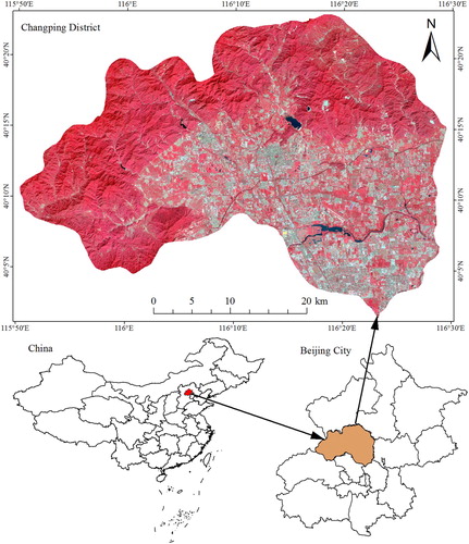
Landsat-8 imagery collected on 4 September 2014 was downloaded from the website https://glovis.usgs.gov/, and an 8-band set of the OLI data was used in this study (i.e. band1 coastal, band2 blue, band3 green, band4 red, band5 nir, band6 swir1, band7 swir2, and band9 cirrus). Moreover, data from the Advanced Spaceborne Thermal Emission and Reflection Radiometer Global Digital Elevation Model (ASTER GDEM) were obtained from the website http://reverb.echo.nasa.gov/reverb/. The ASTER GDEM data are presented as geographic coordinates with a resolution of 1 arcsecond. After projection into UTM and nearest-neighbor resampling, the projection system and resolution of the ASTER GDEM were consistent with those of the Landsat-8 imagery. Together with spectral information, DEM and the slope calculated from DEM were taken as variables in the subsequent classification process.

3. Methods

3.1 Image segmentation

As the first and critical step in object-based image analysis, image segmentation gathers image pixels into segments via the principle of homogeneity in one or more dimensions of a feature space (Blaschke 2010). Several segmentation algorithms have been applied to remote sensing imagery classification (Kartikeyan, Sarkar, and Majumder 1998; Blaschke, Burnett, and Pekkarinen 2004; Wieland and Pittore 2014). In this study, we used the MRS algorithm, one of the most successful segmentation algorithms for segmenting imagery, with eCognition 9.0 software (2014). The MRS algorithm controls the size and shape of segments using three parameters: segmentation scale, shape, and compactness. The segmentation scale parameter determines the maximum criteria of the homogeneity relative to the weighted image layers employed to generate objects, and a greater segmentation scale value results in larger objects. The shape and compactness parameters define the shape of objects by controlling their spectral homogeneity and textural homogeneity, respectively. For segmentation scale, taking into account a large segmentation scale could generate mixed object, we eventually choose 80 as the maximum size of segmentation scale by visual inspection. For shape and compactness, in eCognition software, the value ranges of these two parameters are [0, 0.9] and [0,1], respectively. Finally, in view of the cost of running time, we examined 8 values for the scale parameter (i.e. 10, 20, 30, 40, 50, 60, 70, and 80), 10 values for the shape parameter (i.e. 0, 0.1, 0.2, 0.3, 0.4, 0.5, 0.6, 0.7, 0.8, and 0.9), and 11 values for the compactness parameter (i.e. 0, 0.1, 0.2, 0.3, 0.4, 0.5, 0.6, 0.7, 0.8, 0.9, and 1).

3.2 Classification

3.2.1 Selection of training and testing samples and accuracy evaluation

During pixel-based classification, some researchers suggest a training sample size consisting of at least 10–30 times the number of features (Piper 1987; Mather and Koch 2011). Van Niel, McVicar, and Datt (2005) found that, for a relatively easy classification task, samples of about 2–4 times the number of features were needed to achieve the same accuracy attained using the recommended sample size (i.e. 10–30 times the number of features) with the maximum likelihood classifier. In object-based classification, however, no previous studies have investigated the relationship between sample size and number of features. Bo and Ding (2010) proved that the training sample size required for object-based classification (2–3 times the number of features) is far below that required for pixel-based classification. Considering that the classification problem in this study is uncomplicated and that the distribution of some classes (e.g. grass and water) is scarce, which impedes further sample selection. Finally, we selected 70 training samples, which approximate 2–3 times the number of features, for each class using Google Earth.

For testing samples, we collected samples for each class in proportion to their area ratio. According to statistical data and a preliminary land cover map created with the unsupervised ISODATA clustering algorithm in ENVI 5.1, we roughly estimated the area ratio of each land cover type: forest = 47%, farm = 23%, impervious surface = 22%, grass = 6%, and water = 2%. Then, we collected 690 testing samples, including 300 samples for forest, 150 samples for farm, 150 samples for impervious surface, 50 samples for grass, and 40 samples for water.

Furthermore, we employed a useful statistical indicator, overall accuracy (OA), which was defined as the quotient of the total correct testing samples and the total number of testing samples, to evaluate classification results (Congalton 1991), and used the Z-statistics (Congalton and Mead 1986) to evaluate the significance of OA difference between different classifiers. The OA difference is not significant at the 95% confidence level when the absolute value of the Z-statistics is less than 1.96. A specific mathematical description of Z-statistics can be found in Song, Duan, and Jiang (2012).

3.2.2 Features and feature selection

Since the object-based approach can generate numerous features, we experimented with 134 features that are frequently used by researchers (Wieland and Pittore 2014; Ma et al. 2015). These features were calculated based on the eight spectral bands of the OLI data described above and organized into three groups: spectral measures, geometrical measures, and textual measures. The spectral measures included mean value, standard deviation, ratio, min pixel value, max pixel value, brightness, max difference, normalized difference vegetation index (NDVI), normalized difference built-up index (NDBI), and normalized difference water index (NDWI). The geometrical measures included area, length, length-to-width ratio, number of pixels, volume, width, asymmetry, border index, compactness, density, elliptic fit, radius of largest enclosed ellipse, radius of smallest enclosing ellipse, rectangular fit, roundness, and shape index. The textural measures included gray level co-occurrence matrix (GLCM) homogeneity, GLCM contrast, GLCM dissimilarity, GLCM entropy, GLCM ang. 2nd moment, GLCM mean, GLCM std. dev., and GLCM correlation (Table 1). The detailed specifications of these features can be found in the eCognition manual (Trimble Documentation eCognition® Developer 2014).

Table 1. Object features used for classification.

Feature Type	Object Features	Description
Spectral	mean value^a, standard deviation^a, ratio^a, min pixel value^a, max pixel value^a, brightness, max difference, NDVI, NDBI, NDWI	Spetral features are used to describe image objects with information derived from their spectral properties.
Geometrical	area, length, length-to-width ratio, number of pixels, width, asymmetry, border index, compactness, density, elliptic fit, radius of largest enclosed ellipse, radius of smallest enclosing ellipse, rectangular fit, roundness, shape index	Geometrical features are built on an object’s shape and calculated from the pixels that form it.
Textural	GLCM homogeneity^a, GLCM contrast^a, GLCM dissimilarity^a, GLCM entropy^a, GLCM ang. 2nd moment^a, GLCM mean^a, GLCM std. dev^a, GLCM correlation^a	Textural features originate from Haralick, Shanmugam, and Dinstein (1973) based on the Gray-Level Co-occurrence Matrix.

^aObject features were calculated for each of the 8 multispectral bands mentioned above.

A large number of features that may contain redundant or irrelevant information can result in poor performance of the classifier and increase the computation time (Hall and Holmes 2003; Pedergnana et al. 2013; Wieland and Pittore 2014). Thus, it is necessary to filter features prior to the classification. As a powerful open-source tool, the data mining software Weka 3.8 can be operated on any computer as long as a Java runtime environment has been installed, and it also has a user-friendly graphical user interface that make it easy to use. Hence, in this study, this software was employed to assess the importance of each feature and find an optimal subset of features. First, the ReliefFAttributeEval (ReliefF) method, which is able to generate sorted features (Wieland and Pittore 2014; Ma et al. 2017b), was used to rank all of the features. Using this method, a feature whose values of instances exhibit variance in the same class is given a low-quality score; by contrast, if the feature values of instances are dissimilar in different classes, a high-quality score is assigned to this feature. Then, the CfsSubsetEval (Cfs) method, which has been verified an appropriate approach to select feature subset and has fast processing speed (Hall and Holmes 2003; Ma et al. 2017a, 2017b), was adopted to obtain an optimal features subset. The principle behind this method is that the worth of a features subset is evaluated by considering both the individual predictive ability of each feature and the degree of intercorrelation between them. A subset of features that are greatly correlated with the class but not with each other was selected thereafter. A thorough mathematical description of this method can be found in Hall and Holmes (2003).

3.2.3 Classifiers and parameterizations

According to the statistics (Ma et al. 2017b), classifiers commonly used in related studies mainly include nearest neighbour (NN), support vector machine (SVM), random trees (RT), decision tree (DT), maximum likelihood (ML), and naive Bayes (NB). In this study, four frequently used and built-in classifiers within eCognition were used: SVM, RT, DT, and NB.

As an important tool in data mining, classification and regression trees (CART) was built on a mathematical theory originally introduced by four statisticians in 1984 (Breiman et al.). CART is a type of decision tree (DT) created by several rules grounded on features from the instances. First, rules based on the values of the features are chosen to acquire the optimal split and distinguish instances based on classes. Once a rule is selected, a node is split into two sub-nodes, and the same procedure is applied to each child node. Splitting ceases when all of the instances at a node belong to the same class. Finally, a pruning technique is applied to diminish the size of the DT by eliminating sectors exerting minimal effects when classifying instances. Pruning moderates the influence of overfitting and improves the stability of the classifier. In CART, the maximum depth of the tree has been proven to be a key tuning parameter (Qian et al. 2015); thus, we examined the effect of maximum depth at values from 1 to 15 for all eight segmentation scales.

SVM, also known as support vector networks (Cortes and Vapnik 1995), was first presented by Vapnik (Burges 1998). SVM can implement complex classification by constructing an optimal hyperplane with the kernel function. This optimal hyperplane presents the maximum distance to the closest samples of any class, thereby allowing good separation in different classes. For the kernel function in this study, we chose the frequently used radial basis function (RBF) (Pal and Foody 2010; Faris et al. 2017). Two tuning parameters, C and gamma, are required for the SVM classifier using the RBF kernel in eCognition. C is a penalty parameter, and larger values of C result in more penalties for forecast errors, which means the model may be over-fitted. The value of gamma affects the classification accuracy by controlling the shape of the separating hyperplane (Huang, Davis, and Townshen 2002). Therefore, we examined 10 values for each of these two parameters to investigate how they influence the performance of SVM. The specific values of C are 10⁻¹, 10⁰, 10¹, 10², 10³, 10⁴, 10⁵, 10⁶, 10⁷, and 10⁸, and the values of gamma are 10⁻⁵, 10⁻⁴, 10⁻³, 10⁻², 10⁻¹, 10⁰, 10¹, 10², 10³, and 10⁴.

RT or random forests, which comprise a multitude of DT classifiers, were originally introduced by Leo Breiman (2001). The construction procedure of trees in RT partially differs from that in DT. First, all trees are trained with the same number of samples but on different samples that are obtained from the original sample set. Next, a randomly selected subset of features, rather than all the features, is utilized to detect the optimal split at each node of all trees, and its quantity is constant for any node of any tree. Eventually, each of the trees in RT isn’t pruned compared with pruning process of DT, and a class label of an input feature vector is assigned according to the majority of votes generated from the classification result of every tree. Thus, the size of features and number of trees are clearly two key tuning parameters that must be considered when we use the RT classifier (Wieland and Pittore 2014; Ma et al. 2015). In eCognition software, active variables (n) and maximum tree number (k) are the two parameters we consider. In this research, we tested n values ranging from 1 to 20 and k values ranging from 10 to 100 with increments of 10.

NB is a classic probabilistic classifier based on Bayes’ theorem. It has a long history as a plain but efficient classification method (Good 1966) and assumes that features are independent of each other. In this technique, the means and variances of the features are calculated according to the training samples and then used for classification. Details of the mathematical description of the NB algorithm can be found in the literature (Rish 2001; Zhang, Peña, and Robles 2009). An advantage of the NB classifier over the three other classifiers investigated in this work is that it does not require us to set any tuning parameters.

4. Results

4.1 ReliefF and Cfs results

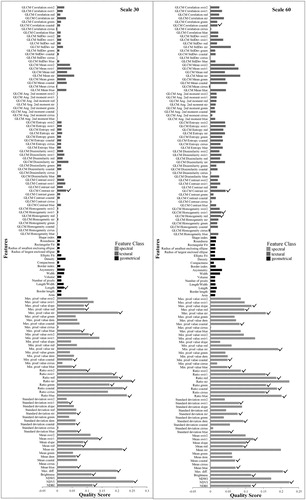
We analyzed the importance of each feature according to the ReliefF and Cfs methods and obtained the optimal features subset at different segmentation scales. Due to the similar patterns obtained at different segmentation scales, we only present herein the results of segmentation scales of 30 and 60 (Figure 2). In Figure 2, the larger the quality score value, the more important the corresponding feature; a checkmark signifies that the feature is contained in the optimal subset. Based on the quality score, we found that the importance of spectral features was obviously higher than that of geometrical and textural features. In terms of the average quality score of each feature group, spectral features accounted for 71%, geometrical features accounted for 12%, and textural features accounted for 17%. The results of the Cfs method revealed that features with high importance may not belong to the optimal features subset (e.g. the minimum pixel value NIR at the segmentation scale of 30 and the mean NIR at the segmentation scale of 60), while features with low importance may (e.g. length at the segmentation scale of 30 and GLCM contrast NIR at the segmentation scale of 60). This results reveals a strong correlation among selected features. In addition, the quantities of features in the optimal subset are 30 and 31 at the segmentation scales of 30 and 60, respectively, and these features are not identical at different segmentation scales. Such a finding indicates that appropriate features must be selected at different segmentation scales.

Figure 2. Importance of the features based on the ReliefF method and Cfs results at the segmentation scales of 30 and 60. (Here, a checkmark means that the feature is included in the optimal subset).

4.2 Effects of segmentation parameters on classification accuracy

To evaluate the influence of segmentation parameters on classification accuracy, we classified the selected image using four classifiers to determine their OA. Figure 3 demonstrates the results we obtained at segmentation scales of 30 and 60 with different combinations of shape and compactness. OA did not show regular changes with increasing value of compactness when the value of shape was fixed. By contrast, the variation in OA presented different patterns at different segmentation scales as the value of shape increased when the value of compactness was fixed. At the segmentation scale of 30, OA displayed small values when the value of shape was low. However, at the segmentation scale of 60, OA presented relatively high values when the value of shape was low. Statistically, at the segmentation scale of 30, the OAs of DT, SVM, RT, and NB varied from 86.4% to 94.8%, 96.2% to 98.3%, 95.1% to 97.8%, and 93.9% to 95.9%, respectively, with different combinations of shape and compactness. At the segmentation scale of 60, the OAs of DT, SVM, RT, and NB fluctuated from 87.5% to 93.9%, 94.9% to 98%, 94.6% to 97.5%, and 91.7% to 95.9%, respectively. In addition, in terms of average OA calculated from all OAs at each fixed value of shape, we obtained the values of shape corresponding to the maximum average OA and the minimum average OA. In the same way, we acquired the values of the parameter compactness (Table 2).

Figure 3. Overall accuracy of the four classifiers with different combinations of shape and compactness at segmentation scales of 30 and 60.

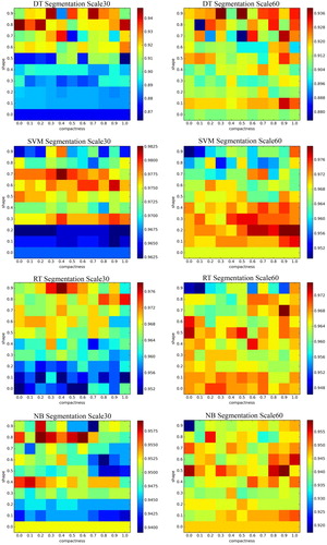
Table 2. Values of shape and compactness corresponding to Max A and Min A with different classifiers.

Classifiers	Max OA				Min OA
	Segmentation Scale30		Segmentation Scale60		Segmentation Scale30		Segmentation Scale60
	S	C	S	C	S	C	S	C
DT	0.8	0.8	0.9	0.9	0	0.6	0.6	0.5
SVM	0.7	0.4	0.2	1	0.2	0.8	0.8	0
RT	0.9	0.3	0\0.5	1	0.1	1	0.9	0.1
NB	0.8	0.2	0.5	1	0.1	1	0.9	0

Note: Max OA: maximum average overall accuracy; Min OA: minimum average overall accuracy; S: shape; and C: compactness.

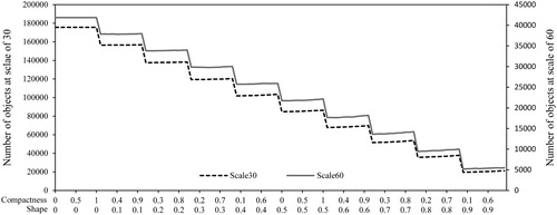
We found that the values of shape corresponding to the maximum average OAs of the classifiers decreased as the segmentation scale increased, except for DT, and that the value of shape corresponding to the minimum average OAs increased as the scale increased. Variations in compactness presented the opposite trend. Thus, a relatively low value of shape and a high value of compactness should be selected as the segmentation scale increases. We then considered the variation in object quantity with different combinations of shape and compactness (Figure 4) and found that the number of objects decreased as the value of shape increased. The maximum object quantity was about nine times the minimum object quantity, and the values of compactness caused minimal impact to the object quantity when the value of shape was fixed. Considering that less time is necessary for classification with lower object quantities, a large value of shape should be selected for segmenting images under the condition of pure objects containing only one type of land cover.

Figure 4. Number of objects at segmentation scales of 30 and 60 with different combinations of shape and compactness.

Figure 5 shows variations in the OAs of the four classifiers as the segmentation scale size increases from 10 to 80. Overall, the OAs first increased and then decreased with increasing segmentation scale size. When the OA reached its maximum value, the segmentation scale values of DT, SVM, RT, and NB were 40, 30, 30/40, and 20, respectively. Moreover, the OAs of DT, SVM, RT, and NB varied from 92.8% to 95.1%, 97.2% to 98.3%, 96.4% to 97.8%, and 94.9% to 96.4%, respectively. We found that the minimum OAs of SVM and RT were larger than the maximum OAs of DT and NB; among the classifiers, SVM showed the best OA, followed by RT, NB, and DT. In addition, based on the optimized classification results made with different classifiers, the Z-statistics (Table 3) indicated that the OA differences between SVM and NB, SVM and DT, and RT and DT were statistically significant, while that between SVM and RT, RT and NB, and NB and DT were not significant.

Figure 5. Overall accuracy of the four classifiers with increasing segmentation scale size.

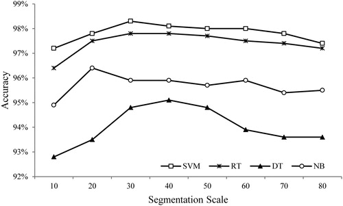
Table 3. Z-statistics of the classification results.

Pair comparsion	SVM vs RT	SVM vs NB	SVM vs DT	RT vs NB	RT vs DT	NB vs DT
Z-statistics	0.7681	2.1832^a	3.5664^a	1.4343	2.8483^a	1.4427

^aSignificant difference at the 95% confidence level.

4.3 Effects of the tuning parameters of the classifiers on classification accuracy

The performance of a classifier can be affected by the tuning parameters within it (Pradhan 2013; Naghibi, Ahmadi, and Daneshi 2017), and Qian et al. (2015) have discussed the influence of tuning parameters on classification accuracy using very high resolution images (0.5 m). Thus, we investigated the impacts of tuning parameters on classification accuracy with imagery of relatively coarse resolution. Because NB classifier is no need to set any tuning parameters, we discussed the effects of tuning paremeters of the other three classifiers on classification accuracy. Taking the segmentation scale value described above at which the OA reached its maximum value, the OAs of DT, SVM, and RT fluctuated from 52.8% to 95.1%, 46.4% to 98.3%, and 95.1% to 97.8%, respectively, under different tuning parameter settings. This result shows that RT is insensitive to the tuning parameters, while DT and SVM are affected by them.

Figures 6–8 present variations in the OAs of DT, SVM, and RT, respectively, under the influence of different tuning parameter settings. Table 4 then shows the optimal parameter values for these three classifiers at different sizes of segmentation scale. For DT, the OA changed significantly when the value of maximum depth was lower than 4. When maximum depth was between 4 and 8, only slight variations in OA were observed, and, when maximum depth was great than or equal to 8, a steady OA was obtained. In general, the optimal maximum depth ranged from 5 to 8.

Figure 6. Overall accuracy of a decision tree with increasing maximum depth values at different segmentation scale sizes.

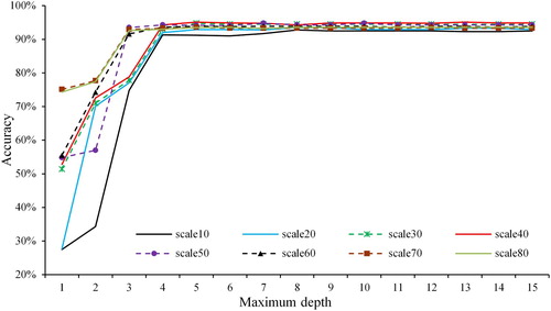
Figure 7. Overall accuracy of a support vector machine with different values of C and gamma at different segmentation scale sizes.

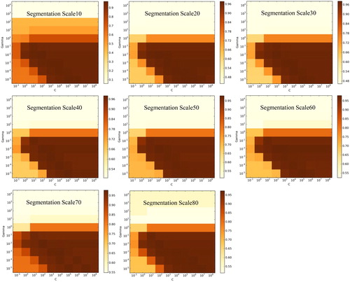
Figure 8. Overall accuracy of a random tree with different values of k and n at different segmentation scale sizes.

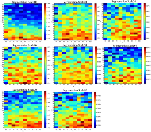
Table 4. Optimal parameter values for three classifiers at different segmentation scale sizes.

Scale	DT	SVM	RT
	Maximum depth	(Gamma, C)	(n, k)
10	8	(10^−2,10^2)	(2,50)
20	8/9	(10^−2,10^2)	(1,40)
30	5	(10^−4,10^4)/(10^−5,10^5)	(4,90)
40	5/13	(10^−2,10^2)	(1,60)
50	7	(10^−2,10^2)	(2,70)
60	5/7-10/12-13/15	(10^−210^2)/(10^−2,10^3)	(2,50)
70	5	(10^−210^2)	(2,30)
80	6/8-15	(10^−4,10^6)	(1,40)/(2,80)/(4,80)/(15,50)/(15,100)

For SVM, as shown in Figure 7, similar patterns of OA could be obtained by using different combinations of tuning parameters at eight sizes of segmentation scale. On the one hand, provided the value of gamma was great than 10⁻¹, regardless of the value of C, the OAs obtained were comparatively small and varied from 5.9% to 81.6%. This finding demonstrates that gamma should less than or equal to 10⁻¹, which is in accordance with the results of Qian et al. (2015). On the other hand, when gamma was between 10⁻⁵ and 10⁻¹ and C was between 10³ and 10⁸, the OAs obtained were relatively high and stable (greater than 90%). In addition, the optimal values of gamma and C were identical, (10⁻², 10²) at the segmentation scales of 10, 20, 40, 50, and 70, and either (10⁻⁴, 10⁴) or (10⁻⁵, 10⁵), (10⁻², 10²) or (10⁻², 10³), and (10⁻⁴, 10⁶) at segmentation scales of 30, 60, and 80, respectively.

Figure 8 demonstrates that the OA of RT basically decreased with increasing n when the value of k was fixed; OA further revealed no obvious regular changes with increasing k when the value of n was fixed, regardless of the scale size. This result indicates that the performance of RT is mainly affected by the value of n. The optimal tuning parameters of RT varied at different sizes of scale. Table 2 reveals that the optimal k varied from 30 to 100 while the optimal n varied mainly from 1 to 4.

5. Discussion

When using an object-based approach, image segmentation, feature selection, and classifiers can markedly influence classification efficiency and accuracy (Duro, Franklin, and Dubé 2012; Qian et al. 2015). In this study, we described the selection of features and investigated the effect of image segmentation and classifiers on classification using Landsat-8 OLI data. The results revealed that spectral features are the most significant factors affecting class separability and that geometrical and textural features have a low and equal relative importance in the classification task (Figure 2). A study by Wieland and Pittore (2014) similarly demonstrated that whereas spectral features are highly important, textual features are more important than geometrical features. This result may be attributed to the different land cover types used in each study, i.e. five types were identified in our study compared with the two identified by Wieland and Pittore (2014). Moreover, Ma et al. (2015) found textural and spectral features to have equal relative importance. This finding may be attributed to the use of images with different resolutions (i.e. a very high-resolution image was used by Ma, whereas we used one with a medium resolution).

In terms of image segmentation, an initial increase and subsequent decrease in OA were observed as the size of the scale increased (Figure 5). Low scale values are well known to generate small objects (Clinton et al. 2010; Myint et al. 2011), which means that a large number of objects accordingly require a large number of training samples to train the classifier. Therefore, when we used the same number of training samples at different segmentation scales, the OA showed an increasing trend. The decreasing trend that was found may be due to the fact that increases in the segmentation scale size attenuate the quality of the samples and deteriorate the classification results (Li et al. 2014); to address this issue, we ensured the quality of the samples by visual inspection. We also investigated the influences of parameter shape and compactness on classification. The results (Figure 3) show that a low shape value and high compactness are preferred as the segmentation scale increases. We also found (Figure 4) that the shape value obviously affects the object’s quantity as well as the segmentation scale value. Thus, when segmenting an image, both the segmentation scale value and the shape value should be carefully considered.

We discussed the influence of different classifiers and the tuning parameters within them for classification accuracy. The results (Figure 5) show that SVM outperforms other classifiers, and this result is in good agreement with the conclusions of Qian et al. (2015) and Kaszta et al. (2016). To achieve the best classification result, we must find the optimal tuning parameters for each classifier, with the exception of NB , which does not require the setting of tuning parameters. Qian et al. (2015) investigated the effect of tuning parameters on classification using very high-resolution images, but few studies that have used medium-resolution images exist. In this paper, we determined the influence of tuning parameters using medium-resolution images. For SVM, setting gamma between 10⁻⁵ and 10⁻¹ and C between 10³ and 10⁸ generally resulted in a high OA. This result is different from that found by Qian et al. (2015) (gamma: 10⁻⁵–10⁻³, C: 10⁶–10⁸) and could be attributed to the different image types are used. Despite this contradiction, however, we found that a comparatively low gamma value and high C value were preferred for SVM. For DT, the optimal maximum depth, which ranges from 5 to 8, is the same as that obtained by Qian et al. (2015), thereby indicating that this range is suitable for similar classification tasks using images with different spatial resolutions. For RT, a small number of active variables usually achieves a high OA, which is in accordance with Rodriguez-Galiano et al.’s (2012) suggestion. Moreover, the suggested number of trees in Rodriguez-Galiano’s study is larger than that in our work. This finding may be due to several reasons: (1) In Rodriguez-Galiano’s research, a single variable (i.e. n = 1) in the RF classifier was used to classify the image; (2) The pixel-based approach was adopted in Rodriguez-Galiano; and (3) Thirteen land cover types were identified in Rodriguez-Galiano’s study, whereas only five types were identified in our study.

In this study, by considering feature selection, image segmentation, and classifiers, we provide meaningful suggestions for land cover classification using medium-resolution images and an object-based approach. However, we conducted this experiment using fixed training samples at different segmentation scales and have yet to study the effect of the size of the training samples on classification accuracy. We will study this topic in future and focus on the applicability of our results to other areas and complex recognition tasks.

6. Conclusions

Using object-based image analysis, classification of Landsat-8 imagery was implemented using four commonly used classifiers (i.e. DT, SVM, RT, and NB), and the effects of segmentation (i.e. scale, shape and compactness) and tuning parameters within these classifiers on OA were discussed. Changes in compactness had little effect on OA when the value of shape was fixed, whereas changes in shape exerted some impact on OA when the value of compactness was fixed. Generally, a low OA could be achieved using a small shape at a minor segmentation scale, and a relatively high OA could be achieved using a small shape at a larger segmentation scale. The tuning parameters of DT and SVM exerted a more significant impact on OA compared with those of RT, and there were significant difference in classification accuracy between SVM and NB, SVM and DT, and RT and DT, while there were no significant difference between SVM and RT, RT and NB, and NB and DT. In general, SVM performed slightly better than the other three classifiers. For DT, the maximum depth should not be less than 5. For SVM, a high OA could be achieved by a gamma between 10⁻⁵ and 10⁻¹ and a C between 10³ to 10⁸. The OA of RT was consistently greater than 90% regardless of the settings of its tuning parameters. Finally, a subset of optimal features was efficiently found using the Cfs method, and the optimal features at different segmentation scales were observed to be non-identical. In summary, tuning parameters exert a greater influence than segmentation parameters on OA. This research provides valuable information for classification using medium-resolution image via the object-based approach.

Acknowledgements

This work was supported by National Key R&D Program of China [2017YFB0503805]; Special Project on High Resolution of Earth Observation System for Major Function Oriented Zones Planning [00-Y30B14-9001-14/16]. Sincere thanks are given for the comments and contributions of anonymous reviewers and members of the editorial team.

Disclosure statement

No potential conflict of interest was reported by the author.

Additional information

Funding

This work was supported by National Key R&D Program of China [2017YFB0503805]; Special Project on High Resolution of Earth Observation System for Major Function Oriented Zones Planning [00-Y30B14-9001-14/16].

References

- An, Kai, Jinshui Zhang, and Yu Xiao. 2007. “Object-oriented Urban Dynamic Monitoring—A Case Study of Haidian District of Beijing.” Chinese Geographical Science 17 (3): 236–242. doi:10.1007/s11769-007-0236-1.
- Blaschke, T. 2010. “Object Based Image Analysis for Remote Sensing.” ISPRS Journal of Photogrammetry and Remote Sensing 65 (1): Elsevier B.V.: 2–16. doi:10.1016/j.isprsjprs.2009.06.004.
- Blaschke, T., C. Burnett, and A. Pekkarinen. 2004. New Contextual Approaches Using Image Segmentation for Object-Based Classification. Dordrecht: Kluver Academic Publishers.
- Bo, Shukui, and Ling Ding. 2010. “The Effect of the Size of Training Sample on Classification Accuracy in Object-Oriented Image Analysis.” Journal of Image and Graphics 15: 1106–1111. (in Chinese) doi:10.11834/jig.20100708.
- Breiman, Leo. 2001. “Random Forests.” Machine Learning 45 (1): 5–32. doi:10.1023/A:1010933404324.
- Breiman, L. I., Jerome H. Friedman, R. A. Olshen, and C. J. Stone. 1984. “Classification and Regression Trees (CART).” Biometrics 40: 358. doi:10.2307/2530946.
- Burges, C. J. C. 1998. “A Tutorial on Support Vector Machines for Pattern Recognition.” Data Mining and Knowledge Discovery 2: 121–167. doi:10.1023/A:1009715923555.
- Clinton, Nicholas, Ashley Holt, James Scarborough, Li Yan, and Peng Gong. 2010. “Accuracy Assessment Measures for Object-Based Image Segmentation Goodness.” Photogrammetric Engineering & Remote Sensing 76 (3): 289–299. doi:10.14358/PERS.76.3.289.
- Congalton, Russell G. 1991. “A Review of Assessing the Accuracy of Classifications of Remotely Sensed Data.” Remote Sensing of Environment 37 (1): 35–46. doi:10.1016/0034-4257(91)90048-B.
- Congalton, Russell G., and Roy A. Mead. 1986. “A Review of Three Discrete Multivariate Analysis Techniques Used in Assessing the Accuracy of Remotely Sensed Data From Error Matrices.” IEEE Transactions on Geoscience and Remote Sensing GE-24 (1): 169–174. doi:10.1109/TGRS.1986.289546.
- Cortes, Corinna, and Vladimir Vapnik. 1995. “Support-Vector Networks.” Machine Learning 20 (3): 273–297. doi:10.1023/A:1022627411411.
- Duro, Dennis C., Steven E. Franklin, and Monique G. Dubé. 2012. “A Comparison of Pixel-Based and Object-Based Image Analysis with Selected Machine Learning Algorithms for the Classification of Agricultural Landscapes Using SPOT-5 HRG Imagery.” Remote Sensing of Environment 118 ( Elsevier Inc): 259–272. doi:10.1016/j.rse.2011.11.020.
- Estoque, Ronald C, Yuji Murayama, and Chiaki Mizutani Akiyama. 2015. “Pixel-Based and Object-Based Classifications Using High- and Medium-Spatial-Resolution Imageries in the Urban and Suburban Landscapes.” Geocarto International 30 (10): 1113–1129. doi:10.1080/10106049.2015.1027291.
- Faris, Hossam, Mohammad A. Hassonah, Ala’ M. Al-Zoubi, Seyedali Mirjalili, and Ibrahim Aljarah. 2017. “A Multi-Verse Optimizer Approach for Feature Selection and Optimizing SVM Parameters Based on a Robust System Architecture.” Neural Computing and Applications no. January. Springer London: 1–15. doi:10.1007/s00521-016-2818-2.
- Good, I. J. 1966. “The Estimation of Probabilities: an Essay on Modern Bayesian Methods.” Biometrics 23 (1): 158–161. doi:10.2307/2528296.
- Hall, M. A., and Geoffrey Holmes. 2003. “Benchmarking Attribute Selection Techniques for Discrete Class Data Mining.” IEEE Transactions on Knowledge and Data Engineering 15 (6): 1437–1447. doi:10.1109/TKDE.2003.1245283.
- Haralick, Robert M., K. Shanmugam, and I. Dinstein. 1973. “Textural Features for Image Classification.” IEEE Transactions on System, Man and Cybernetics SMC-3 (6): 610–621. doi: 10.1109/TSMC.1973.4309314
- Huang, Chengquan, L. S. Davis, and J. R. G. Townshen. 2002. “An Assessment of Support Vector Machines for Land Cover Classification.” International Journal of Remote Sensing 23 (4): 725–749. doi:10.1080/01431160110040323.
- Joshi, Neha, Matthias Baumann, Andrea Ehammer, Rasmus Fensholt, Kenneth Grogan, Patrick Hostert, Martin Rudbeck Jepsen, et al. 2016. “A Review of the Application of Optical and Radar Remote Sensing Data Fusion to Land Use Mapping and Monitoring.” Remote Sensing 8 (1): 1–23. doi:10.3390/rs8010070.
- Kartikeyan, B., A. Sarkar, and K. L. Majumder. 1998. “A Segmentation Approach to Classification of Remote Sensing Imagery.” International Journal of Remote Sensing 19 (9): 1695–1709. doi:10.1080/014311698215199.
- Kaszta, Zaneta, Ruben Van De Kerchove, Abel Ramoelo, Moses Azong Cho, Sabelo Madonsela, Renaud Mathieu, and Eléonore Wolff. 2016. “Seasonal Separation of African Savanna Components Using WorldView-2 Imagery: A Comparison of Pixeland Object-Based Approaches and Selected Classification Algorithms.” Remote Sensing 8 (9): 763. doi:10.3390/rs8090763.
- Li, Manchun, Lei Ma, Thomas Blaschke, Liang Cheng, and Dirk Tiede. 2016. “A Systematic Comparison of Different Object-Based Classification Techniques Using High Spatial Resolution Imagery in Agricultural Environments.” International Journal of Applied Earth Observation and Geoinformation 49: 87–98. doi:10.1016/j.jag.2016.01.011.
- Li, Congcong, Jie Wang, Lei Wang, Luanyun Hu, and Peng Gong. 2014. “Comparison of Classification Algorithms and Training Sample Sizes in Urban Land Classification with Landsat Thematic Mapper Imagery.” Remote Sensing 6 (2): 964–983. doi:10.3390/rs6020964.
- Ma, Lei, Liang Cheng, Wenquan Han, Lishan Zhong, and Manchun Li. 2014. “Cultivated Land Information Extraction from High-Resolution Unmanned Aerial Vehicle Imagery Data.” Journal of Applied Remote Sensing 8 (1): 083673. doi:10.1117/1.JRS.8.083673.
- Ma, Lei, Liang Cheng, Manchun Li, Yongxue Liu, and Xiaoxue Ma. 2015. “Training Set Size, Scale, and Features in Geographic Object-Based Image Analysis of Very High Resolution Unmanned Aerial Vehicle Imagery.” ISPRS Journal of Photogrammetry and Remote Sensing 102: International Society for Photogrammetry and Remote Sensing, Inc. (ISPRS): 14–27. doi: 10.1016/j.isprsjprs.2014.12.026
- Ma, Lei, Tengyu Fu, Thomas Blaschke, Manchun Li, Dirk Tiede, Zhenjin Zhou, Xiaoxue Ma, and Deliang Chen. 2017a. “Evaluation of Feature Selection Methods for Object-Based Land Cover Mapping of Unmanned Aerial Vehicle Imagery Using Random Forest and Support Vector Machine Classifiers.” ISPRS International Journal of Geo-Information 6 (2): 51. doi:10.3390/ijgi6020051.
- Ma, Lei, Manchun Li, Xiaoxue Ma, Liang Cheng, Peijun Du, and Yongxue Liu. 2017b. “A Review of Supervised Object-Based Land-Cover Image Classification.” ISPRS Journal of Photogrammetry and Remote Sensing 130: 277–293. doi:10.1016/j.isprsjprs.2017.06.001.
- Mather, Paul M., and Magaly Koch. 2011. Computer Processing of Rmeotely-Sensed Images. 4th ed. Chichester: Wiley-Blackwell.
- Myint, Soe W., Patricia Gober, Anthony Brazel, Susanne Grossman-Clarke, and Qihao Weng. 2011. “Per-Pixel vs. Object-Based Classification of Urban Land Cover Extraction Using High Spatial Resolution Imagery.” Remote Sensing of Environment 115 (5): Elsevier Inc.: 1145–1161. doi:10.1016/j.rse.2010.12.017.
- Naghibi, Seyed Amir, Kourosh Ahmadi, and Alireza Daneshi. 2017. “Application of Support Vector Machine, Random Forest, and Genetic Algorithm Optimized Random Forest Models in Groundwater Potential Mapping.” Water Resources Management 31 (9): 2761–2775. doi:10.1007/s11269-017-1660-3.
- Pal, M. 2005. “Random Forest Classifier for Remote Sensing Classification.” International Journal of Remote Sensing 26 (1): 217–222. doi:10.1080/01431160412331269698.
- Pal, M., and G. M. Foody. 2010. “Feature Selection for Classification of Hyperspectral Data by SVM.” IEEE Transactions on Geoscience and Remote Sensing 48: 2297–2307. doi:10.1109/TGRS.2009.2039484.
- Pedergnana, Mattia, Prashanth Reddy Marpu, Mauro Dalla Mura, Jón Atli Benediktsson, and Lorenzo Bruzzone. 2013. “A Novel Technique for Optimal Feature Selection in Attribute Profiles Based on Genetic Algorithms.” IEEE Transactions on Geoscience and Remote Sensing 51 (6): 3514–3528. doi: 10.1109/TGRS.2012.2224874
- Petropoulos, George P., Charalambos Kontoes, and Iphigenia Keramitsoglou. 2011. “Burnt Area Delineation From a Uni-Temporal Perspective Based on Landsat TM Imagery Classification Using Support Vector Machines.” International Journal of Applied Earth Observation and Geoinformation 13 (1): Elsevier B.V.: 70–80. doi:10.1016/j.jag.2010.06.008.
- Piper, J. 1987. “The Effect of Zero Feature Correlation Assumption on Maximum Likelihood Based Classification of Chromosomes.” Signal Processing 12: 49–57. doi:10.1016/0165-1684(87)90081-8.
- Platt, Rutherford V, and Lauren Rapoza. 2008. “An Evaluation of an Object- Oriented Paradigm for Land Use/Land Cover Classification an Evaluation of an Object-Oriented Paradigm for Land Use/Land Cover Classification.” The Professional Geographer 60: 87–100. doi:10.1080/00330120701724152.
- Pradhan Biswajeet. 2013. “A Comparative Study on the Predictive Ability of the Decision Tree, Support Vector Machine and Neuro-Fuzzy Models in Landslide Susceptibility Mapping Using GIS.” Computer and Geosciences 51: 350–365. doi:10.1016/j.cageo.2012.08.023.
- Pu, Ruiliang, Shawn Landry, and Qian Yu. 2011. “Object-Based Urban Detailed Land Cover Classification with High Spatial Resolution IKONOS Imagery.” International Journal of Remote Sensing 32 (12): 3285–3308. doi:10.1080/01431161003745657.
- Qian, Yuguo, Weiqi Zhou, Jingli Yan, Weifeng Li, and Lijian Han. 2015. “Comparing Machine Learning Classifiers for Object-Based Land Cover Classification Using Very High Resolution Imagery.” Remote Sensing 7 (1): 153–168. doi:10.3390/rs70100153.
- Rish, Irina. 2001. “An Empirical Study of the Naive Bayes Classifier.” IJCAI 2001 Workshop on Empirical Methods in Artificial Intelligence 3 (January 2001): 41–46.
- Rodriguez-Galiano, V. F., B. Ghimire, J. Rogan, M. Chica-Olmo, and J. P. Rigol-Sanchez. 2012. “An Assessment of the Effectiveness of a Random Forest Classifier for Land-Cover Classification.” ISPRS Journal of Photogrammetry and Remote Sensing 67: 93–104. doi:10.1016/j.isprsjprs.2011.11.002.
- Song, Xianfeng, Zheng Duan, and Xiaoguang Jiang. 2012. “Comparison of Artificial Neural Networks and Support Vector Machine Classifiers for Land Cover Classification in Northern China Using a SPOT-5 HRG Image.” International Journal of Remote Sensing 33 (10): 3301–3320. doi: 10.1080/01431161.2011.568531
- Trimble Documentation eCognition® Developer 9.0 Reference Book. 2014. München, Germany.
- Van Niel, Thomas G., Tim R. McVicar, and Bisun Datt. 2005. “On the Relationship between Training Sample Size and Data Dimensionality: Monte Carlo Analysis of Broadband Multi-Temporal Classification.” Remote Sensing of Environment 98 (4): 468–480. doi:10.1016/j.rse.2005.08.011.
- Wieland, Marc, and Massimiliano Pittore. 2014. “Performance Evaluation of Machine Learning Algorithms for Urban Pattern Recognition from Multi-Spectral Satellite Images.” Remote Sensing 6 (4): 2912–2939. doi:10.3390/rs6042912.
- Wieland, Marc, Yolanda Torres, Massimiliano Pittore, and Belen Benito. 2016. “Object-Based Urban Structure Type Pattern Recognition from Landsat TM with a Support Vector Machine.” International Journal of Remote Sensing 37 (17): 4059–4083. doi:10.1080/01431161.2016.1207261.
- Wu, Hao, Zhiping Cheng, Wenzhong Shi, Zelang Miao, and Chenchen Xu. 2014a. “An Object-Based Image Analysis for Building Seismic Vulnerability Assessment Using High-Resolution Remote Sensing Imagery.” Natural Hazards 71 (1): 151–174. doi:10.1007/s11069-013-0905-6.
- Wu, Hao, Lu-Ping Ye, Wen-Zhong Shi, and Keith C. Clarke. 2014b. “Assessing the Effects of Land Use Spatial Structure on Urban Heat Islands Using HJ-1B Remote Sensing Imagery in Wuhan, China.” International Journal of Applied Earth Observation and Geoinformation 32 (October). Elsevier B.V.: 67–78. doi:10.1016/j.jag.2014.03.019.
- Yan, Gao J. F. Mas, B. H. P. Maathuis, X. Zhang, and P. M. G. Van Dijk. 2006. “Comparison of Pixel-Based and Object-Oriented Image Classification Approaches—A Case Study in a Coal Fire Area, Wuda, Inner Mongolia, China.” International Journal of Remote Sensing 27 (18): 4039–4055. doi: 10.1080/01431160600702632
- Yu, Qian, Peng Gong, Nick Clinton, Greg Biging, Maggi Kelly, and Dave Schirokauer. 2006. “Object-Based Detailed Vegetation Classification with Airborne High Spatial Resolution Remote Sensing Imagery.” Photogrammetric Engineering & Remote Sensing 72 (7): 799–811. doi:10.14358/PERS.72.7.799.
- Zhang, Min Ling, José M. Peña, and Victor Robles. 2009. “Feature Selection for Multi-Label Naive Bayes Classification.” Information Sciences 179 (19): 3218–3229. doi:10.1016/j.ins.2009.06.010.