A scalable cyberinfrastructure and cloud computing platform for forest aboveground biomass estimation based on the Google Earth Engine

ABSTRACT

Earth observation (EO) data, such as high-resolution satellite imagery or LiDAR, has become one primary source for forests Aboveground Biomass (AGB) mapping and estimation. However, managing and analyzing the large amount of globally or locally available EO data remains a great challenge. The Google Earth Engine (GEE), which leverages cloud-computing services to provide powerful capabilities on the management and rapid analysis of various types of EO data, has appeared as an inestimable tool to address this challenge. In this paper, we present a scalable cyberinfrastructure for on-the-fly AGB estimation, statistics, and visualization over a large spatial extent. This cyberinfrastructure integrates state-of-the-art cloud computing applications, including GEE, Fusion Tables, and the Google Cloud Platform (GCP), to establish a scalable, highly extendable, and high-performance analysis environment. Two experiments were designed to demonstrate its superiority in performance over the traditional desktop environment and its scalability in processing complex workflows. In addition, a web portal was developed to integrate the cyberinfrastructure with some visualization tools (e.g. Google Maps, Highcharts) to provide a Graphical User Interfaces (GUI) and online visualization for both general public and geospatial researchers.

KEYWORDS:

• Above ground biomass
• cloud computing
• Google Earth Engine
• visualization

1. Introduction

Forests play a critically important role in the global carbon cycle by serving as a major carbon (C) sink through photosynthesis and a C emission source due to deforestation, forest clearing, or change of land use (Houghton 2005). Quantifying forest C storage involves the calculation of forest biomass – the total biological materials of food, fiber, and fuel wood (Amidon et al. 2008). It is also well recognized that forest biomass changes can greatly affect biodiversity, the hydrological system, soil degradation, as well as other ecosystem functions (D’Almeida et al. 2007; Verschuyl et al. 2011; Liu et al. 2012). The integrated conversation, management, and utilization of forest biomass may lead to production of environment-friendly renewable fuels, a key element in mitigating greenhouse gas emissions and optimizing the balance across energy security, economic growth, and the environment (Bartuska 2006). Therefore, accurate measurement of the biomass across local, regional, even global scales carries significant meaning for understanding its roles in environment changes and sustainable development (Foody, Boyd, and Cutler 2003; Lu et al. 2016).

Forest biomass consists of aboveground (e.g. stems, branches, leaves) biomass and belowground (e.g. roots) biomass. Most studies have focused on the aboveground biomass (AGB) due to the difficulty in acquiring data belowground (Lu et al. 2016). Field measurement, as one classic method for AGB estimation, is deemed to be most accurate (Lu et al. 2016). However, it is time-consuming, expensive, and labor-intensive, and therefore difficult to apply to a large-scale study (Zolkos, Goetz, and Dubayah 2013; Chen et al. 2016; Lu et al. 2016). In comparison, remote sensing can rapidly capture multiple forest features important to biomass calculation consistently over large spatial extents, such as canopy height and stem width. Its advantages in large coverage, high spatial-temporal resolution, digital encoding, etc., make it a primary choice for large-scale AGB mapping and estimation (Lu et al. 2016).

While remote sensing data, such as LiDAR (Light Detection and Ranging), has become increasingly available to support biomass analysis (Lee et al. 2011), the massive amount of data and its complex data structure pose great challenges in data storage and computation (Li, Hodgson, and Li 2018). Traditional LiDAR-based approach is difficult to scale due to the intensive nature for point-based analysis. Tools developed are always desktop-based and they are specific to certain software and operating system, making them difficult to be reused. Cloud computing, a new high performance computing paradigm designed to tackle computation-intensive problems, becomes a promising solution technique (Yang et al. 2010; Zhang et al. 2016). In recent years, many researchers from various scientific fields have adopted cloud computing to tackle big data problems by utilizing its advantage in scalable computing capability, on-demand resource allocation, and low hardware maintainence cost (Keahey et al. 2008). Yet to the best of our knowledge, there is no study that has been conducted to exploit cloud computing for AGB estimation. In addition, traditional cloud computing platforms only provide a computing environment where all the configurations, data and applications need to be built by researchers. It also requires an in-depth understanding in computing in order to optimize resource allocation and system performance. How to rapidly develop an efficient application to handle the data and computation challenges in LiDAR-based AGB estimation is a big challenge.

In this paper, we exploited a feasible cloud computing method to solve the intensive computational challenges in the analysis of massive remotely sensed data for AGB estimation. A scalable cyberinfrastructure was developed to integrate cloud computing, existing powerful cloud applications (e.g. GEE, Fusion Tables), and visualization tools (e.g. Google Maps, Highcharts) for high performance computation and effective visual analytics. The contributions of this work are: (1) a new big data management mechanism for effectively organizing and storing diverse dataset, including LiDAR data, high-resolution satellite images, vector boundary data etc., is introduced; (2) the AGB estimation algorithm is parallelized and accelerated by a GEE-based cloud computing platform; (3) a cyberinfrastructure portal is developed to allow interactive AGB query, statistics, and visualization. The sections are organized as follows: section 2 reviews earlier scientific applications on GEE. Section 3 introduces the scalable cyberinfrastructure (CI) framework for AGB estimation. Section 4 describes the critical aspects of the framework. Section 5 illustrates the implementation of the CI portal and demonstrates the portal’s performance and scalability through two experiments. The last section concludes the work and proposes some potential research points in the future.

2. Literature review

2.1. Spatial cloud computing

Rapid advancement of spatial data acquisition methods (e.g. Earth Observation, unmanned aerial vehicles, LiDAR scanner) results in the production of a massive amount of geospatial data (Yang et al. 2010; Romero et al. 2011), requiring therefore a new way to store, organize and process these resources. Cloud computing, a computing paradigm that adopts the concept of elastic resource allocation and virtualization has been proposed to directly address these computing needs for big data analytics (Li et al. 2016). Cloud computing platforms provide computing resources by service-oriented abstraction, including Infrastructure as a Service (IaaS), Platform as a Service (PaaS) and Software as a Service (SaaS) (Mell and Grance 2011). Several open source cloud computing software, such as CloudStack (Kumar et al. 2014), and OpenStack (Sabharwal and Shankar 2013; Lamourine 2014) have been widely used to establish the institutional or private cloud (Wuhib, Stadler, and Lindgren 2012, Tan et al. 2015). There are also many popular commercial cloud platforms, i.e. Microsoft Azure, Google Cloud Platform, Amazon Web Services (AWS), available to allow researchers to rapidly deploy applications and conduct experiments. Although readily available, these platforms only provide a computing environment, all the configurations, data and applications need to be built by researchers. It also requires an in-depth understanding in computing in order to optimize resource allocation and system performance. To further provide an integrated and easy-to-use environment for scientific analysis, Google has released its GEE platform, where scientists are allowed to have ‘local’ access to various datasets, and achieve parallel programing using GEE built-in library without a steep learning curve on parallelism, resource scheduling and allocation. GEE also provides supporting cloud services for data storage, exchange and indexing, further facilitating problem solving especially when big data is used. These advantages make GEE an ideal platform for most users, especially scientists in different disciplines to rapidly construct their own cloud-based high-performance applications.

As sensor technology and remote sensing has improved, massive amounts of data with various data structures have been collected, raising grand challenges to traditional data management. For example, increasing data volume requires data management systems to be scalable in storage capability. The diversity in data structures requires new strategies to support heterogeneous data storage. Although many solutions have been proposed to tackle the above challenges, such as the use of parallel file systems (e.g. Lustre, OrangeFS, HDFS) and NoSQL database (e.g. HBase, MongoDB) (Borthakur 2008; Zhao et al. 2010; George 2011; Yang, Ligon, and Quarles 2011; Almeer 2012; Chodorow 2013; Ma et al. 2015), they often require a complicated system-level integration and configuration of data storage and access tools, processing modules, as well as visualization interface. The complexity for developing such systems are very high. In comparison, GEE platform provides a one-stop cloud service for enabling scientific analysis, including GEE data catalog hosting vast amount of remote sensing data for image processing and analysis, Google Fusion Table (Gonzalez et al. 2010) for importing application-specific datasets, as well as its built-in API to support elastic computing and parallel processing. Therefore, we chose GEE as the cyberinfrastructure framework for large-scale biomass estimation.

2.2. Google Earth Engine

Google Earth Engine (GEE), as a cloud-based platform enabling planetary-scale geospatial data management and analysis, provides users with access to massive historical EO data, scientific algorithms, and powerful computing capability (Moore and Hansen 2011). It has been collecting satellite images for more than 40 years and manages them with all original data and metadata, including the complete data of Landsat 4, 5, 7 and 8 from the United States Geological Survey (USGS), Moderate Resolution Imaging Spectroradiometer (MODIS) datasets, and some other scientific datasets (Padarian et al. 2015). Users can also upload their local data for processing in GEE. In addition, GEE, as an intrinsically parallel image-processing platform, provides many optimized algorithms which can automatically distribute the computation tasks across many CPUs in Google’s cloud infrastructure (Lobell et al. 2015). Thanks to the above advantages, GEE has attracted much attention from various scientific fields (e.g. biology, geography, hydrology) as the big data era arrives (Hansen et al. 2013; Edmonds et al. 2016; Goldblatt et al. 2016; Soulard et al. 2016).

The rich historical EO datasets make it easier to conduct temporal series analysis. Hansen et al. (2013) analyzed global forest cover changes between 2000 and 2012 using the Landsat dataset. Soulard et al. (2016) assessed effects of wildfires on meadows in Yosemite National Park between 1985 and 2012 based on the Landsat 5 images. Edmonds et al. (2016) studied the flow path of river avulsion channels in the Andean and Himalayan foreland basins between 1984 and 2014 using Landsat images. Okoro et al. (2016) used the Landsat 5, 7 and 8 images to monitor oil palm land cover changes in the Niger delta.

Several other studies were carried out by utilizing GEE’s powerful computation capability. Hansen et al. (2013) achieved global forest mapping and change detection at a 30 m resolution from 2000 to 2012. This study demonstrated the powerful calculation potential of GEE. Lobell et al. (2015) mapped crop yield using GEE to rapidly process a large volume of historical Landsat and weather images. Soulard et al. (2016) used GEE to manage the challenges in data storage and computational efficiency when they assessed the role of climate and resource management on ground water dependent ecosystem changes in arid environments. All these studies showcased GEE’s great potential in handling the challenges in intensive imagery organization and computation for AGB estimation.

GEE also provides a series of data mining and analysis algorithms to enhance its analytical capability. Patel et al. (2015) and Goldblatt et al. (2016) directly used its built-in classifiers, such as the Support Vector Machines (SVM), Random Forest (RF) and classification and regression trees (CART), to map the multi-temporal settlement and population of the Indonesian island of Java, as well as the extraction of urban areas in India. However, there was some sacrifice in the results accuracy because of some limitations in GEE’s built-in algorithms (Patel et al. 2015). To avoid this shortcoming, Lobell et al. (2015) just used the GEE as one step to map the crop yield in the Midwestern United States. Dong et al. (2016) developed their phenology-and-pixel-based paddy rice mapping (PPPM) algorithm in GEE to analyze the paddy rice area in northeastern Asia. Taking advantage of the analytical capability of GEE, the process for developing new AGB algorithms can be greatly accelerated.

GEE provides two approaches for users to access its data and computational resources (Houghton et al. 2001; Moore and Hansen 2011). One is the web-based Integrated Development Environment (IDE) Earth Engine Code Editor where users can edit, manage, and run their algorithms. The other is the Application Programming Interface (API) which can be used to develop new applications. However, the GEE is still a programing tool, which creates an inevitably long learning curve for common users. To ease the use of GEE, Yalew, van Griensven, and van der Zaag (2016) developed a suite of interactive web-tools (AgriSuit) to integrate various spatial datasets and local desktop software (e.g. QGIS) to assess the regional environment on top of GEE. In this tool, while algorithms and data types are enriched, the entire workflow was split into separate components, and the massive data transmission among different components decreases the efficiency.

In this paper, we propose and develop a cloud-based online CI platform for AGB estimation. We utilize various state-of-the-art cloud applications for development of scalable AGB estimation algorithms, cloud management of big data, and deployment of the web portal. This effective utilization of cloud-based resources eases integration effort, reduces communication overhead, and allows a world-wide access to the scalable cyberinfrastructure.

3. Architecture

As shown in Figure 1, the proposed cyberinfrastructure framework for AGB estimation is built by leveraging the Google Cloud Platform and some other advanced cloud applications. There are six loosely coupled components from bottom to up: Google Cloud Platform, computation module, cloud-based spatial database module, visualization tools, AGB application server, and web portal.

Figure 1. Cloud-based cyberinfrastructure for AGB estimation.

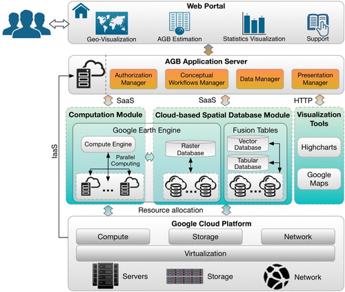
The web portal provides all interactive functions through the Graphical User Interfaces (GUI). Specifically, (1) Geo-visualization works as the main presentation window which allows users to render geospatial data and analytical results on the base map; (2) AGB estimation services enable users to quantify AGB values and errors across different scales (e.g. pixel-level, area-level) at different spatial resolutions; (3) The statistics visualization module can assist users in analyzing the AGB results by dynamically producing multiple statistics graphs such as bar graph, pie graph, error bar graph; (4) The support module presents users with some basic description about our system, including the study area and data, AGB algorithms, user manual, etc.

The AGB application server works as a bridge between the web portal and cloud services. First, it receives users’ requests from the web portal. Then, the incoming requests are parsed and sent to corresponding cloud application services for further processing. Finally, processing results are retrieved and presented in the relevant widget in the web portal. There are four important managers designed to support users’ operations in the portal: (1) Authorization manager maintains the authorization files required by third-party applications, such as the service account and private key for GEE. (2) Conceptual workflows manager maintains the logical workflows for AGB estimation. When users request the AGB estimation, AGB workflow will be enabled in the GEE compute engine. (3) Data manager supports many data operations, such as data query, format conversion, download, based on the backend spatial database. (4) Presentation manager initializes the web portal and dynamically changes graphical interfaces responding to users’ operations. It also invokes some cloud-based visualization tools to display data and analytical results.

The cloud-based spatial database management and computation modules are the core of this framework to tackle the challenges in big data storage and computation. The former serves as the container of massive heterogeneous spatial data for AGB estimation. Raster data, such as elevation data derived from LiDAR data, is managed by the raster data engine as part of the GEE. Vector data, such as county or state boundaries, as well as non-spatial tabular data is managed by the Fusion Tables. The high-performance computation module provides scalable computation capabilities using GEE’s compute engine to parallelize computation tasks to run across distributed servers in the Google cloud platform.

These two modules integrate and provides cloud services in the form of SaaS (Software as a Service). The Google cloud platform, on the other hand, provides Infrastructure as a Service (IaaS) for supporting on-demand allocation of computing resources (e.g. CPU, storage, network). The IaaS mechanism releases us from investment and efforts in maintaining physical machines.

Visualization tools are used to initialize portal interfaces and visualize geospatial data, results, and their statistical graphs, which are integrated with the entire framework through the presentation manager in the AGB application server. Two popular tools, Google Maps and Highcharts, were adopted to achieve the above functions because they provide rich visualization capability and can be easily integrated into our platform.

4. Methodology

4.1. Study area and data

The study area is located in northeastern Minnesota (Figure 2) which covers roughly 65,000 km². The majority of this area is covered by forests composed of softwood trees and hardwood trees. Dominant tree species in this area include quaking aspen, balsam fir, black spruce, paper birch, black ash, northern white-cedar, red maple, and jack pine (Chen et al. 2016). The large forest coverage and diverse plant types make it a challenging and important location for AGB estimation, which is why it was selected as our study area.

Figure 2. The study area in northeastern Minnesota.

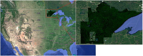
Two datasets have been collected in this study. One is the vector administrative boundary for Minnesota from the U.S. Census Bureau which includes county and census tracts boundaries. The other is the canopy quadric mean height metric image for the study area (source: Chen et al. 2016). The raw data was rasterized at the spatial resolution of 13 m by 13 m from the native LiDAR points collected between 2011 and 2012. The raster image was divided into more than eight thousand GeoTiff (Ritter et al. 2000) files using the USGS quadrangle system.

4.2. Cloud-based management of big spatial data

As described in section 2, GEE is a cloud-based platform enabling planetary-scale geospatial data management and analysis. It provides two important components for raster data management: asset manager and public data catalog. The asset manager allows users to upload raster files as GeoTiffs and organizes them in one unique directory created for a specific user. To guarantee data privacy, the uploaded data is configured as private by default. Additionally, users can also share their data by configuring ‘write’ or ‘read’ permission to other groups or individuals. The public data catalog shares massive earth science raster images with a temporal coverage of over 40 years with all GEE users. Fusion Tables is another cloud-based service to support management, visualization, and sharing of tabular data in multiple formats, such as Comma Separated Values (CSV), Keyhole Markup Language (KML), spreadsheets, etc. It shares similar mechanisms for data privacy control as the asset manager of GEE. Fusion Tables also provides users with a keyword-based search mechanism for the public tables shared by different organizations or applications, which can be used as a complementary data source for research. Another advantage of Fusion Tables is that it has a spatial extension to store geometry data in addition to textual data. Shapefiles, for example, can be uploaded and managed as a cloud dataset using this application. In addition, the GEE asset manager and Fusion Tables are built upon Google’s cloud infrastructure, making them scalable to manage big data. These nice features make Fusion Tables an appealing application for cloud data management.

In this study, the canopy height metric images were uploaded into the data directory in the asset manager and organized as an image collection using the earth engine code editor. Then they can be accessed through the image collection’s unique identifier. Each original image file is cut into tiles and image pyramid is established to store sub-image areas at multiple resolutions to support fast data access and filtering. The public data catalog, containing Landsat or other images in time-series, is used as an external data source to support research, such as providing historical image views of the study area. The vector boundary datasets were first transformed into Keyhole Markup Language (KML), and then uploaded as data tables in Fusion Tables. These datasets can be accessed worldwide by specifying their unique name/identifier on the cloud. This way, cloud-based, scalable management of raster and vector data are implemented.

4.3. Efficient AGB estimation based on GEE

4.3.1. Algorithms description

There have been many algorithms developed to estimate AGB for different tree species in various study areas. The algorithm developed by Chen et al. (2016) was selected because it is capable of estimating both AGB and uncertainty across different scales (pixel, area) and spatial resolutions. Equations (1–5) list the formula for calculating pixel-level AGB, which is the basis for area-level AGB estimation.(1) $B_{\mathrm{p}\mathrm{i}\mathrm{x}}={\beta }_1{h}_{qm}^{{\beta }_2}$(1) (2) ${\sigma }_{\epsilon ,\mathrm{p}\mathrm{i}\mathrm{x}}^2=(\theta B_{\mathrm{p}\mathrm{i}\mathrm{x}}{)}^2$(2) (3) ${\sigma }_{f,\mathrm{p}\mathrm{i}\mathrm{x}}^2=\sum _{p=1}^2\sum _{q=1}^2\left(\overline{g_{p,\mathrm{p}\mathrm{i}\mathrm{x}}}\text{cov}\right({\beta }_p,{\beta }_q\left)\overline{g_{q,\mathrm{p}\mathrm{i}\mathrm{x}}}\right)$(3) (4) ${\sigma }_{z,\mathrm{p}\mathrm{i}\mathrm{x}}^2=({\theta }^2+1)(0.1\ast {\beta }_2{B}_{\mathrm{p}\mathrm{i}\mathrm{x}}{)}^2$(4) (5) ${\sigma }_{\mathrm{p}\mathrm{i}\mathrm{x}}=\sqrt[2]{{\sigma }_{\epsilon ,\mathrm{p}\mathrm{i}\mathrm{x}}^2+{\sigma }_{f,\mathrm{p}\mathrm{i}\mathrm{x}}^2+{\sigma }_{z,\mathrm{p}\mathrm{i}\mathrm{x}}^2}$(5)

Where $B_{\mathrm{p}\mathrm{i}\mathrm{x}}$ represents the AGB value of a single pixel, $h_{qm}$ is the quadric mean height of points within the pixel which can be directly read from the canopy height metric image, and ${\beta }_1$ and ${\beta }_2$ are model parameters calculated by Chen et al. (2016); ${\sigma }_{\epsilon ,\mathrm{p}\mathrm{i}\mathrm{x}}$, ${\sigma }_{f,\mathrm{p}\mathrm{i}\mathrm{x}}$, and ${\sigma }_{z,\mathrm{p}\mathrm{i}\mathrm{x}}$ are errors of pixel-level AGB that result from the residual variance, parameters estimation, and canopy height metric, respectively. ${\sigma }_{\mathrm{p}\mathrm{i}\mathrm{x}}$ is the total error of pixel-level AGB. $\theta$ is a parameter related to model residuals, p and q are indices for model parameter $\beta$, $\overline{g_{p,\mathrm{p}\mathrm{i}\mathrm{x}}}$ is the Jacobian value of ${\beta }_p$which equals $\mathrm{\partial }{B}_{\mathrm{p}\mathrm{i}\mathrm{x}}/\mathrm{\partial }{\beta }_p$.(6) ${\mu }_{\mathrm{a}\mathrm{r}\mathrm{e}\mathrm{a}}=\frac{1}{N}\sum _{i=1}^N{B}_{\mathrm{p}\mathrm{i}\mathrm{x}}$(6) (7) ${\sigma }_{\epsilon ,\mathrm{a}\mathrm{r}\mathrm{e}\mathrm{a}}^2=\frac{1}{N^2}\sum _{i=1}^N{\sigma }_{\epsilon ,\mathrm{p}\mathrm{i}\mathrm{x},i}^2$(7) (8) ${\sigma }_{f,\mathrm{a}\mathrm{r}\mathrm{e}\mathrm{a}}^2=\sum _{p=1}^2\sum _{q=1}^2(\overline{g_{p,\mathrm{a}\mathrm{r}\mathrm{e}\mathrm{a}}}\text{cov( }{\beta }_p,{\beta }_q)\overline{g_{q,\mathrm{a}\mathrm{r}\mathrm{e}\mathrm{a}}})$(8) (9) ${\sigma }_{z,\mathrm{a}\mathrm{r}\mathrm{e}\mathrm{a}}^2=\frac{1}{N^2}\sum _{i=1}^N{\sigma }_{z,\mathrm{p}\mathrm{i}\mathrm{x},i}^2$(9) (10) ${\sigma }_{\mathrm{a}\mathrm{r}\mathrm{e}\mathrm{a}}=\sqrt[2]{{\sigma }_{\epsilon ,\mathrm{a}\mathrm{r}\mathrm{e}\mathrm{a}}^2+{\sigma }_{f,\mathrm{a}\mathrm{r}\mathrm{e}\mathrm{a}}^2+{\sigma }_{z,\mathrm{a}\mathrm{r}\mathrm{e}\mathrm{a}}^2}$(10) Equations (6–10) further provide formula for calculating area-based AGB. Among which, ${\mu }_{\mathrm{a}\mathrm{r}\mathrm{e}\mathrm{a}}$ is the AGB density in the area, N represents the number of pixels contained in the area, ${\sigma }_{\epsilon ,\mathrm{a}\mathrm{r}\mathrm{e}\mathrm{a}}$, ${\sigma }_{f,\mathrm{a}\mathrm{r}\mathrm{e}\mathrm{a}}$, and ${\sigma }_{z,\mathrm{a}\mathrm{r}\mathrm{e}\mathrm{a}}$ indicate errors of area-level AGB which are related to the residual variance, parameter estimation, and canopy height metric, and ${\sigma }_{\mathrm{a}\mathrm{r}\mathrm{e}\mathrm{a}}$ refers to the total error of area-level AGB. ${\sigma }_{\epsilon ,\mathrm{p}\mathrm{i}\mathrm{x},i}$ refers to the residual variance error of the i-th pixel. $\overline{g_{p,\mathrm{a}\mathrm{r}\mathrm{e}\mathrm{a}}}$ is the average Jacobian value of ${\beta }_p$ in each pixel. $\overline{g_{p,\mathrm{a}\mathrm{r}\mathrm{e}\mathrm{a}}}$ can be calculated using ${\displaystyle \frac{1}{N}\sum _{i=1}^N\left(\mathrm{\partial }{B}_{\mathrm{p}\mathrm{i}\mathrm{x}}/\mathrm{\partial }{\beta }_p\right)}$, and ${\sigma }_{z,\mathrm{p}\mathrm{i}\mathrm{x},i}$ is the LiDAR metric error of the i-th pixel.

In the whole process, the basic calculation unit is pixel-wise analysis. When it comes to the area-based AGB estimation, the process will be divided into two steps: (1) pixel-based AGB estimation, and then (2) an aggregation of all values on the pixels falling inside of the study area. Because there are few interdependency in the computation, this process is extremely well-suited for parallel processing. We can therefore leverage the power of GEE, a cyberinfrastructure optimized to enable planetary-scale image processing (Gorelick et al. 2017) for our application to speed up the computing efficiency.

4.3.2. Implementation of AGB estimation based on GEE

GEE’s compute engine has been optimized for image analysis, which can automatically partition the original image into multiple sub-images and distribute them across many machines for parallel calculation. At the same time, it can dynamically assign the computing resource according to the computational intensity of user requests (Gorelick et al. 2017). The elastic parallelization and compute resource scheduling is therefore automatically achieved. Besides, several optimization strategies are further adopted to improve overall system performance. First, the client variables (defined by developers) and server-side variables (defined according to GEE API specifications) are made consistent such that there is no extra effort needed to conduct the variable-type conversion before the workflow is sent and executed on the GEE server. Second, we enable partial data loading to alleviate memory deficit of the low-end servers that GEE’s underlying infrastructure is actually built on (Gorelick et al. 2017). Third, we group calculations that use the same input data, such that calculations belonging to the same group will be completed on a single pass to save client-server data exchange time.

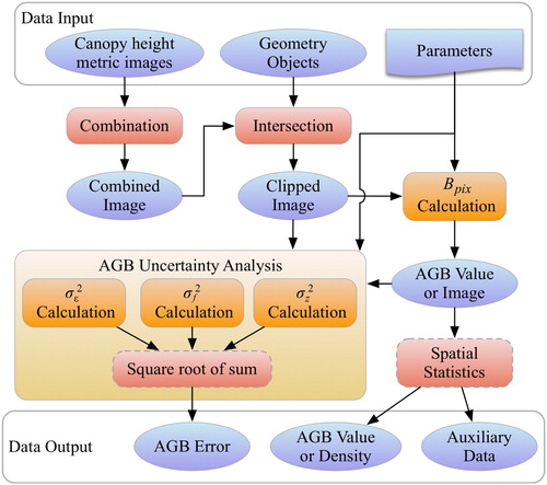
Figure 3 demonstrates the conceptual workflow for AGB estimation in the compute engine, including data combination, intersection, algebraic operations, and spatial statistics. The implementation details are as follows:

1. Combination of canopy height metric image tiles. This step assembles all image tiles into a spatially continuous one. The overlapping pixels across the tiles were also merged. Their order in the collection is used in assigning the value of the overlapping pixels, which means the pixel value in the top (most recent) image is adopted as the final value in the assembled image.

2. Data intersection. This operation obtains the intersection of assembled image with a given study area, so pixels falling outside of the study area is clipped and will not be considered in the data processing.

3. $B_{\mathrm{p}\mathrm{i}\mathrm{x}}$ calculation. Algebraic operations were adopted in this step to achieve Equation (1) for $B_{\mathrm{p}\mathrm{i}\mathrm{x}}$ calculation. Its output can be a single value representing the pixel-level AGB or an image showcasing the area-level AGB.

4. Spatial statistics. This function will be enabled when there is a request for area-level AGB estimation. Max, min, average of the AGB values will be calculated for cross-comparison among multiple areas of interest. In this procedure, a map-reduce model was adopted for faster and parallel data summary.

5. AGB uncertainty analysis. There are three kinds of errors to be estimated (see details in section 4.3.1). The final error is calculated as the square root of the sum of the squared errors.

Figure 3. Conceptual workflows for AGB estimation in GEE.

4.3.3. Caching strategy for AGB values within administrative units

AGB result caching can reduce users’ waiting time by transforming time-costly computing tasks into results’ query. At the same time, it can also free computing resources for other on-the-fly computing tasks. However, whether or not to cache all results and which result to cache are two challenging topics. The increase in cached data volume will lead to lower query efficiency and larger storage cost. Popular results are usually more frequently queried than others, and therefore should be given higher priority for caching. To develop an optimal caching strategy, we first classified the AGB estimation into three levels including pixel level, area level (in any arbitrary boundary), and administrative units’ level. For the AGB results in pixel level, the results’ volume is huge and are even larger than the canopy height metric image. In addition, its calculation is fast enough for users to get results nearly in real time. For the area level AGB results, although their volume is small, their calculations are time-intensive. However, different users always pay attention to different study areas, making area level AGB results a lower popularity query. In contrast, the AGB within administrative units is appealing to nearly all users which can be used for either longitudinal or cross-sectional studies. In addition, the limited number and fixed boundaries of administrative units guarantee small data volume and high query efficiency. In our implementation, we chose to cache all AGB results at the administrative unit level in Fusion Tables.

4.4. System workflows for AGB estimation and visualization

4.4.1. AGB estimation system workflow

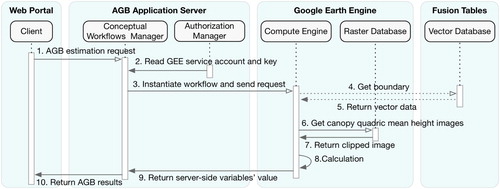
Figure 4 demonstrates the workflow for AGB estimation in our portal. Initially, users specify the model parameters (location of one pixel or boundary of polygons, spatial resolution) in the portal and send requests to AGB application server (step 1). The conceptual workflows manager will be informed to handle the incoming request, which will instantiate one workflow in compute engine using the model parameters and authorization information (service account, key) required by GEE from the authorization manager (step 2, 3). Next, the compute engine will execute the workflow instance and return results. In this process, GEE needs to determine whether to get boundaries from Fusion Tables according to the workflow types. If it is the workflow for AGB estimation within administrative units, the administrative boundary data will need to be retrieved from the Fusion Tables through HTTP requests (step 4, 5). Otherwise, the location or boundary data is contained in the workflow instance. Next, the compute engine will request the clipped canopy quadric mean height image within the location or boundary from the raster database (step 6, 7). Then, GEE will execute the workflow instance (step 8) and return specified variables’ value to conceptual workflows manager in the application server (step 9). Finally, conceptual workflows manager encodes the AGB values together with some other data (e.g. number of pixels, location) and returns them to the end-users (step 10).

Figure 4. Sequence diagram of AGB calculation and uncertainty analysis.

4.4.2. The workflow for visualization of geospatial data and statistics data

Data visualization can foster understanding by presenting data using multiple methods (Li et al. 2016). In this paper, we adopted two existing visualization tools (Google Maps and Highcharts) to visualize the statistical and geospatial data in our portal. It can free users from installing other visualization software on local computers and downloading massive amounts of data. Figure 5 presents the visualization workflows, including raster data visualization, vector data visualization, and statistics data visualization.

Figure 5. Sequence diagram of geospatial and statistics data visualization.

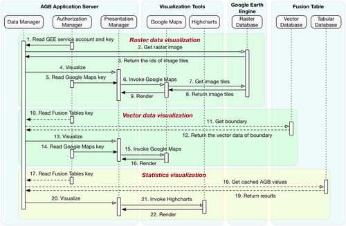
When users select to view the raster data (e.g. canopy height metric image, historical satellite images), the data manager will construct a get image request to the raster database in GEE (step 1, 2). This request contains spatial-temporal parameters provided by users and the authorization information (service account and key) required by GEE from the authorization manager. Once GEE receives the request, it will inform the raster database to filter images using the spatial-temporal restrictions and return the identifications for filtered image tiles (step 3). Then, the presentation manager is invoked to render the image tiles in Google Maps (step 4–9). In this process, Google Maps needs to retrieve the image tiles from the raster database using their unique ids.

Differing from raster data, vector data consists of dynamic data drawn by users on a map and the static data managed in Fusion Tables. For the dynamic vector data, the data manager directly uses the presentation manager to visualize it on Google Maps (step 14–16). However, when users want to visualize the data from Fusion Tables, the data manager needs to first read the vector data from the Fusion Tables (step 10–12), then overlay it on top of Google Maps through its API.

Because of the caching mechanism for administrative AGB, the visualization workflow for statistics data contains two strategies dependent upon the data sources. When requested data is cached in advance, the data manager will directly read its value from the tabular database (step 17–19) and invokes Highcharts to produce statistical graphs (step 20–22). Otherwise, the data manager will wait for the real-time processing results and visualize them using the Highcharts (step 20–22).

5. Implementation and experiments

5.1. Implementation

In this paper, the webapp2 framework was adopted to simplify the development of AGB application server. It uses the Jinja2 and WSGI (Web Server Gateway Interface) to separate the presentation in browsers from the logic models in the backend server (Ronacher 2008; Gardner 2009), which makes the portal more flexible and easier to extend and maintain. The application server is deployed in the Google Cloud Platform through the IaaS which releases us from the investment and time costing in using a physical server. The communications among our application server and other components are based on the API of external applications. An asynchronous strategy based on the Asynchronous JavaScript and XML (AJAX) (Garrett 2005) was used to improve functions’ interactivity between the web portal and the application server.

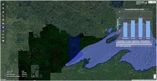
Figure 6 demonstrates the Graphical User Interface (GUI) of the AGB estimation portal that integrates the data transmissions, analysis, and visualization. The menu bar allows users to select all functions provided by our system. The base map, as the main visualization window, is used for users to select an area of interest on the map and then visualize geospatial data and results. Basic map operations (e.g. pan, zoom in/out, basic map changes) are supported to enhance its interactivity. If users want to compare the AGB results among different locations, the error bar graph can be dynamically rendered and displayed on the map as a floating window. There are also some other functions developed to enhance user experience, such as the location selection, historical image view, etc.

Figure 6. The homepage of the web portal (https://biomass-estimation.appspot.com/).

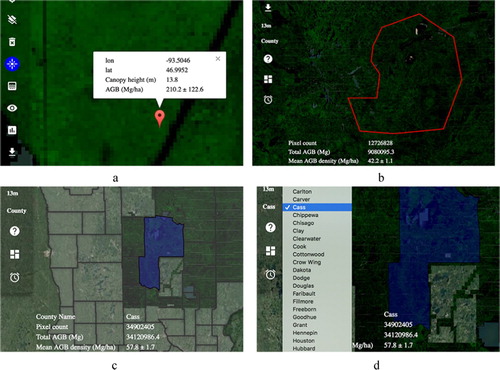
There are several interactive methods for users to select the location for AGB estimation (Figure 7). For the pixel-level AGB, users can directly click on the map to select a pixel and calculate its AGB values and errors (results are shown in Figure 7(a)). If users want to calculate the area-level AGB, there are three methods provided. Users can draw a polygon with any arbitrary boundary for area-based AGB calculation (Figure 7(b)). They can also select an administrative area by clicking it on the map (Figure 7(c)) or selecting its name from the dropdown list (Figure 7(d)).

Figure 7. AGB estimation across different region.

We also developed the historical image view function to assist users in verifying the AGB estimation through visual interpretation. Although the field survey is the most accurate method to verify the AGB estimation, it is always time-consuming, expensive, and labor-intensive. In contrast, historical satellite images provide a very large amount of image data over a large spatial range through a wide range of different time periods which can be used to verify the results of AGB estimation by visual interpretation. In this study, we developed this function using the aerial images of the US at one-meter spatial resolution collected by the US National Agriculture Imagery Program (NAIP). NAIP collects data on a five-year cycle between 2003 and 2008, and on a three-year cycle since 2009. Figure 8 presents the historical images in the part of our study area which is located around 47°33′00N, 91°55′50W to the northwest of Big Lake. By comparing the different views, we determined that forest deforestation started from 2011 in the highlighted regions. If more canopy height metrics become available, we can also calculate the AGB loss by comparing AGB values at different timestamps. Table 1 shows the AGB value in each of the highlighted areas in 2011.

Figure 8. The AGB loss because of deforestation activities.

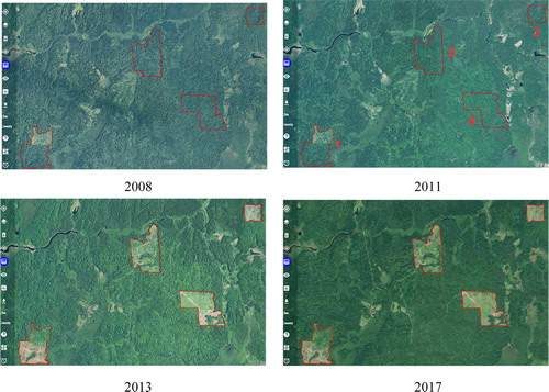
Table 1. AGB values in 2011 in highlighted areas in Figure 8.

Area	Pixel number	AGB (Mg)	Mean AGB density (Mg/ha)
1	2814	5048.4	106.2 ± 4.1
2	3205	981.3	18.1 ± 0.7
3	870	95.7	6.5 ± 0.5
4	3066	5075.6	98 ± 3.1

5.2. Experiment

In this section, we present two experiments to test the system performance for AGB estimation. Experiment 1 compares the performance between the MATLAB implementation and our method as the number of pixels increases. Because users often choose to calculate AGB within ROIs (e.g. state, country), which have complex boundaries, we further exploit the system scalability and performance for regional AGB estimation in Experiment 2. In these experiments, Apache JMeter (Halili 2008) was used to simulate users’ requests and record the response times.

5.2.1. Comparison in performance between MATLAB and our system

In the experiment, we increased the number of pixels by changing the extent of the input image. Figure 9 demonstrates the results for two methods. The x-axis shows the number of pixels in the input image, and the y-axis shows the average response time.

Figure 9. Comparison in compute time between MATLAB and our method.

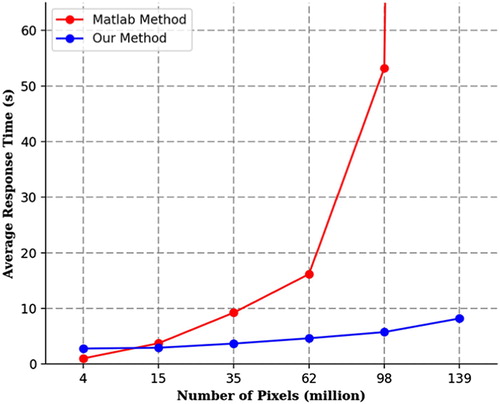
It can be clearly observed that: (1) when there are a small number of pixels, the MATLAB method takes less time than our method. This is because in a web implementation of our method, extra time is required in the network connection and data transmission since the data, application, and users are all distributed. (2) As the number of pixels increases, the response time of MATLAB increases much more sharply than ours. This is not surprising since the computer capabilities are limited in the MATLAB method, while our method can elastically allocate more computing resources and parallelize the computing tasks across them through GEE. (3) There is a significant drop in the efficiency of MATLAB method when the number of pixels exceeds 62 million. This is probably due to the fact that the data size becomes too large for MATLAB to store completely in system memory (RAM). In such cases, data needs to be swapped between system memory and the hard-drive, causing a much longer compute time. These results suggest that our method can effectively handle the intense computational challenges for AGB estimation over large areas.

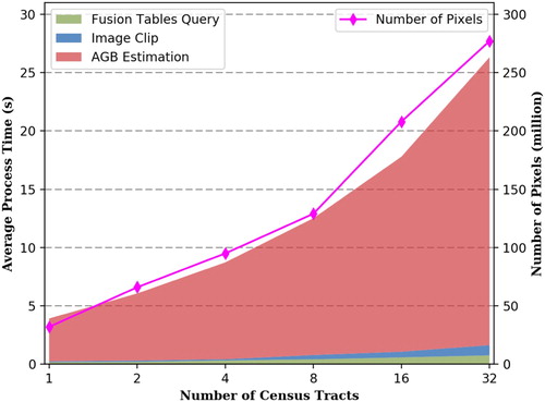
5.2.2. System scalability and performance for regional AGB estimation

While experiment one utilized a pre-clipped image as input, this experiment exploits the system performance for area-level AGB estimation in real situations, which includes vector data query from Fusion Tables, image clip, and AGB estimation. In this section, we tested the time cost in each process phase by computing the regional AGB within multiple census tracts. Figure 10 demonstrates the processing time at different phases and total number of pixels as the number of census tracts increases. As seen in the Figure, the Fusion Tables query and images clip always take very small parts of the total time, suggesting a very small overhead for cloud-based data access and spatial analysis. In addition, GEE achieves the image clip operation by first rasterizing the boundary polygons using the image’s projection with specified resolution, then the rasterized results were used to intersect with the images. This solution substantially accelerated the efficiency of the intersection process. As the number of census tracts increases, the processing time of AGB estimation shows a similar linearly increasing pattern as the results show in Figure 9. Both results show that our system can scale very well in terms of handling big data calculation by dynamically adjusting and allocating needed distributed computing resources.

Figure 10. The comparison of process time with different census tracts’ number.

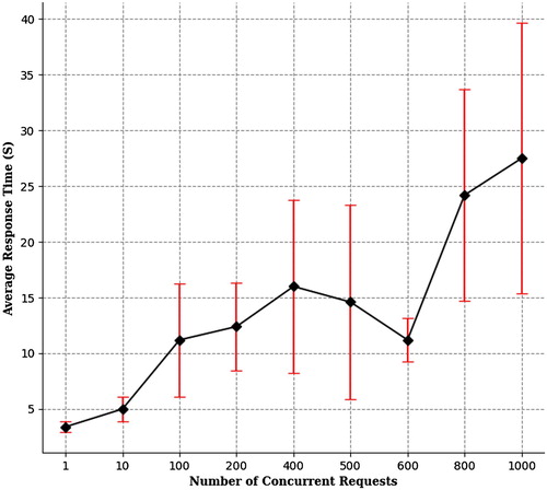
5.2.3. Scalability in handling concurrent user requests

To test the robustness of our system in handling concurrent user access, the processing time with different initial number of requests was recorded and shown in Figure 11. In this experiment, the study area covering [(94°W, 46°N), (93°W, 47°N)] are used for AGB calculation. This study area is estimated to contain 42,450,909 pixels in total. Each experiment was repeated for five times and the response time is an average of the five results. From Figure 11, it can be observed that in general, the processing time increases as the number of requests increases, but the rate of its increase is much slower compared to that of the number of requests. This means the system scales well by automatically assigning more computing resources to handle more incoming requests. We can also observe some instability in this system though, reflected by the drop of processing time at concurrent request number set to 600, and the larger error bar as more concurrent requests come in. A possible reason for this is since GEE is a public rather than dedicated cloud platform, application with more requests may not be prioritized in resource allocation for every of its requests when multiple different applications are competing for the computing resources.

Figure 11. Average processing time as number of concurrent user access increases.

6. Conclusion and future research

This paper proposes and develops a scalable cyberinfrastructure for AGB estimation by integrating cloud computing services and existing state-of-the-art applications for data management, analysis and visualization. The main contributions of the paper are: (1) A new cloud-based data management mechanism for diverse datasets was developed. It integrates GEE asset manager and public data catalog to manage massive raster images, and Fusion Tables to cloud-store vector and tabular data; (2) The AGB estimation was parallelized and accelerated using the Google cloud infrastructure – specifically GEE. Several optimization strategies were adopted to accelerate the entire processes; (3) A web-based portal was developed to provide users with key functions in the GUI, including data transmission, AGB query, statistics, and a spatial visualization. This web portal enables web access, computation, and visualization of AGB, greatly facilitating collaborative research on carbon cycle, deforestation, land use and land cover change, etc. The implementation of our portal also provides a useful reference for cyber-infrastructure researchers in developing cloud-based applications by integrating existing advanced applications. Experiments show that the system achieves high scalability, efficiency, and interactivity.

However, some improvements should be considered in future research. First, we plan to extend our GEE-based AGB estimation to a large-scale, from national- to global-scale studies to benefit the broader science community. A challenge in this is the lack of global LiDAR data due to high cost in data collection (Chen et al. 2016; Lu et al. 2016). Massive amount of remote sensing optical images is available in GEE’s data catalog; however, they often cannot perform AGB estimation as accurate as LiDAR data-based approach because of coarser resolution and weaker height sensitivity in these imageries (Lu et al. 2016). Resolving this issue, we plan to look into the integrated use of LiDAR data and massive amounts of optical images to take advantages of LiDAR data in its high accuracy, and optical images in its global coverage. Machine learning techniques, such as transfer learning, will be applied to achieve high-accuracy and large-scale AGB calculation. Second, as our proposed GEE-based parallel computing framework is generalizable for geospatial raster-based analysis, we plan to extend it for supporting other applications, such as watershed analysis, wildfire damage estimation etc.

Disclosure statement

No potential conflict of interest was reported by the authors.

ORCID

Wenwen Li http://orcid.org/0000-0003-2237-9499

References

- Almeer, M. H. 2012. “Cloud Hadoop Map Reduce for Remote Sensing Image Analysis.” Journal of Emerging Trends in Computing and Information Sciences 3 (4): 637–644.
- Amidon, T. E., C. D. Wood, A. M. Shupe, Y. Wang, M. Graves, and S. Liu. 2008. “Biorefinery: Conversion of Woody Biomass to Chemicals, Energy and Materials.” Journal of Biobased Materials and Bioenergy 2: 100–120. doi: 10.1166/jbmb.2008.302
- Bartuska, A. 2006. Why Biomass is Important: The Role of the USDA Forest Service in Managing and Using Biomass for Energy and Other Uses. Speech Given at 25x25 Summit II, Washington, DC, USA. Accessed 17 July 2018. http://www.fs.fed.us/research/pdf/biomass_importance.pdf.
- Borthakur, D. 2008. “HDFS Architecture Guide.” Hadoop Apache Project, 53.
- Chen, Q., R. E. McRoberts, C. Wang, and P. J. Radtke. 2016. “Forest Aboveground Biomass Mapping and Estimation across Multiple Spatial Scales Using Model-based Inference.” Remote Sensing of Environment 184: 350–360. doi: 10.1016/j.rse.2016.07.023
- Chodorow, K. 2013. MongoDB: The Definitive Guide: Powerful and Scalable Data Storage, 3–27. Sebastopol: O’Reilly Media.
- D’Almeida, C., C. J. Vörösmarty, G. C. Hurtt, J. A. Marengo, S. L. Dingman, and B. D. Keim. 2007. “The Effects of Deforestation on the Hydrological Cycle in Amazonia: A Review on Scale and Resolution.” International Journal of Climatology 27: 633–647. doi: 10.1002/joc.1475
- Dong, J., X. Xiao, M. A. Menarguez, Geli Zhang, Yuanwei Qin, David Thau, Chandrashekhar Biradar, and Berrien Moore. 2016. “Mapping Paddy Rice Planting Area in Northeastern Asia with Landsat 8 Images, Phenology-based Algorithm and Google Earth Engine.” Remote Sensing of Environment 185: 142–154. doi: 10.1016/j.rse.2016.02.016
- Edmonds, D. A., E. A. Hajek, N. Downton, and A. B. Bryk. 2016. “Avulsion Flow-path Selection on Rivers in Foreland Basins.” Geology 44: 695–698. doi: 10.1130/G38082.1
- Foody, G. M., D. S. Boyd, and M. E. J. Cutler. 2003. “Predictive Relations of Tropical Forest Biomass from Landsat TM Data and their Transferability between Regions.” Remote Sensing of Environment 85: 463–474. doi: 10.1016/S0034-4257(03)00039-7
- Gardner, J. 2009. “The Web Server Gateway Interface (Wsgi).” In The Definitive Guide to Pylons, 369–388. New York: Apress.
- Garrett, J. J. 2005. “Ajax: A New Approach to Web Applications.”
- George, L. 2011. HBase: The Definitive Guide: Random Access to Your Planet-size Data, 1–29. Sebastopol: O’Reilly Media.
- Goldblatt, R., W. You, G. Hanson, and A. K. Khandelwal. 2016. “Detecting the Boundaries of Urban Areas in India: A Dataset for Pixel-based Image Classification in Google Earth Engine.” Remote Sensing 8: 634. doi: 10.3390/rs8080634
- Gonzalez, H., A. Y. Halevy, C. S. Jensen, Anno Langen, Jayant Madhavan, Rebecca Shapley, Warren Shen, and Jonathan Goldberg-Kidon. 2010. “Google Fusion Tables: Web-centered Data Management and Collaboration.” Proceedings of the 2010 ACM SIGMOD International Conference on Management of Data, ACM, 1061–1066.
- Gorelick, N., M. Hancher, M. Dixon, S. Ilyushchenko, D. Thau, and R. Moore. 2017. “Google Earth Engine: Planetary-scale Geospatial Analysis for Everyone.” Remote Sensing of Environment 202: 18-27. doi:10.1016/j.rse.2017.06.031.
- Halili, E. H. 2008. “Load/Performance Testing of Website.” In Apache JMeter: A Practical Beginner's Guide to Automated Testing and Performance Measurement for Your Websites, 51–74. Olton: Packt.
- Hansen, M. C., P. V. Potapov, R. Moore, M. Hancher, S. A. Turubanova, A. Tyukavina, D. Thau, et al. 2013. “High-resolution Global Maps of 21st-century Forest Cover Change.” Science 342: 850–853. doi: 10.1126/science.1244693
- Houghton, R. A. 2005. “Aboveground Forest Biomass and the Global Carbon Balance.” Global Change Biology 11 (6): 945–958. doi:10.1111/j.1365-2486.2005.00955.x.
- Houghton, R. A., K. T. Lawrence, J. L. Hackler, and S. Brown. 2001. “The Spatial Distribution of Forest Biomass in the Brazilian Amazon: A Comparison of Estimates.” Global Change Biology 7: 731–746. doi: 10.1046/j.1365-2486.2001.00426.x
- Keahey, K., R. Figueiredo, J. Fortes, T. Freeman, and M. Tsugawa. 2008. “Science Clouds: Early Experiences in Cloud Computing for Scientific Applications.” Cloud Computing and Applications 2008: 825–830.
- Kumar, R., K. Jain, H. Maharwal, N. Jain, and A. Dadhich. 2014. “Apache Cloudstack: Open Source Infrastructure as a Service Cloud Computing Platform.” Proceedings of the International Journal of Advancement in Engineering Technology, Management and Applied Science 1 (2): 111–116.
- Lamourine, M. 2014. “Openstack.” Login:: The Magazine of USENIX & SAGE 39: 17–20.
- Lee, S., W. Ni-Meister, W. Yang, and Q. Chen. 2011. “Physically Based Vertical Vegetation Structure Retrieval from ICESat Data: Validation using LVIS in White Mountain National Forest, New Hampshire, USA.” Remote Sensing of Environment 115 (11): 2776–2785. doi:10.1016/j.rse.2010.08.026.
- Li, W., H. Shao, S. Wang, X. Zhou, and S. Wu. 2016. “A2CI: A Cloud-based, Service-oriented Geospatial Cyberinfrastructure to Support Atmospheric Research.” In Cloud Computing in Ocean and Atmospheric Sciences, edited by T. C. Vance, N. Merati, C. Yang, and M. Yuan, 137–161. London: Elsevier.
- Li, Z., M. E. Hodgson, and W. Li. 2018. “A General-purpose Framework for Parallel Processing of Large-scale LiDAR Data.” International Journal of Digital Earth, 11 (1):26-47. doi:10.1080/17538947.2016.1269842.
- Liu, Y., X. Wei, X. Guo, D. Niu, J. Zhang, X. Gong, and Y. Jiang. 2012. “The Long-term Effects of Reforestation on Soil Microbial Biomass Carbon in Sub-tropic Severe Red Soil Degradation Areas.” Forest Ecology and Management 285: 77–84. doi: 10.1016/j.foreco.2012.08.019
- Lobell, D. B., D. Thau, C. Seifert, E. Engle, and B. Little. 2015. “A Scalable Satellite-based Crop Yield Mapper.” Remote Sensing of Environment 164:324–333. doi:10.1016/j.rse.2015.04.021.
- Lu, D., Q. Chen, G. Wang, L. Liu, G. Li, and E. Moran. 2016. “A Survey of Remote Sensing-based Aboveground Biomass Estimation Methods in Forest Ecosystems.” International Journal of Digital Earth 9 (1): 63–105. doi: 10.1080/17538947.2014.990526
- Ma, Y., H. Wu, L. Wang, Bormin Huang, Rajiv Ranjan, Albert Zomaya, and Wei Jie. 2015. “Remote Sensing Big Data Computing: Challenges and Opportunities.” Future Generation Computer Systems 51: 47–60. doi: 10.1016/j.future.2014.10.029
- Mell, P., and T. Grance. 2011. “The NIST Definition of Cloud Computing.”
- Moore, R., and M. Hansen. 2011. “Google Earth Engine: A New Cloud-computing Platform for Global-scale Earth Observation Data and Analysis.” In AGU Fall Meeting Abstracts, 02.
- Okoro, S. U., U. Schickhoff, J. Bohner, and U. A. Schneider. 2016. “A Novel Approach in Monitoring Land-cover Change in the Tropics: Oil Palm Cultivation in the Niger Delta, Nigeria.” Erde 147: 40–52.
- Padarian, J., B. Minasny, and A. B. McBratney. 2015. “Using Google's Cloud-based Platform for Digital Soil Mapping.” Computers & Geosciences 83:80–88. doi:10.1016/j.cageo.2015.06.023.
- Patel, N. N., E. Angiuli, P. Gamba, A. Gaughan, G. Lisini, F. R. Stevens, A. J. Tatem, and G. Trianni. 2015. “Multitemporal Settlement and Population Mapping from Landsat Using Google Earth Engine.” International Journal of Applied Earth Observation and Geoinformation 35: 199–208. doi: 10.1016/j.jag.2014.09.005
- Ritter, N., M. Ruth, B. B. Grissom, G. Galang, J. Haller, G. Stephenson, S. Covington, T. Nagy, J. Moyers, and J. Stickley. 2000. “GeoTIFF Format Specification GeoTIFF Revision 1.0.” SPOT Image Corp.
- Romero, D. M., W. Galuba, S. Asur, and B. A. Huberman. 2011. “Influence and Passivity in Social Media.” In Joint European Conference on Machine Learning and Knowledge Discovery in Databases, 18–33. Berlin Heidelberg: Springer.
- Ronacher, A. 2008. “Jinja2 Documentation.” Welcome to Jinja2—Jinja2 Documentation (2.8-dev).
- Sabharwal, N., and R. Shankar. 2013. Apache CloudStack Cloud Computing, 17–40. Olton: Packt.
- Soulard, C. E., C. M. Albano, M. L. Villarreal, and J. J. Walker. 2016. “Continuous 1985–2012 Landsat Monitoring to Assess Fire Effects on Meadows in Yosemite National Park, California.” Remote Sensing 8: 371. doi: 10.3390/rs8050371
- Tan, X., L. Di, M. Deng, J. Fu, G. Shao, M. Gao, Z. Sun, X. Ye, Z. Sha, and B. Jin. 2015. “Building an Elastic Parallel OGC Web Processing Service on a Cloud-based Cluster: A Case Study of Remote Sensing Data Processing Service.” Sustainability 7 (10): 14245–14258. doi:10.3390/su71014245.
- Verschuyl, J., S. Riffell, D. Miller, and T. B. Wigley. 2011. “Biodiversity Response to Intensive Biomass Production from Forest Thinning in North American Forests – A Meta-Analysis.” Forest Ecology and Management 261: 221–232. doi: 10.1016/j.foreco.2010.10.010
- Wuhib, F., R. Stadler, and H. Lindgren. 2012. “Dynamic Resource Allocation with Management Objectives—Implementation for an OpenStack Cloud.” Network and Service Management 610: 309–315.
- Yalew, S. G., A. van Griensven, and P. van der Zaag. 2016. “AgriSuit: A Web-based GIS-MCDA Framework for Agricultural Land Suitability Assessment.” Computers and Electronics in Agriculture 128: 1–8. doi: 10.1016/j.compag.2016.08.008
- Yang, S., W. B. Ligon, and E. C. Quarles. 2011. “Scalable Distributed Directory Implementation on Orange File System.” Proc. IEEE Intl. Wrkshp. Storage Network Architecture and Parallel I/Os (SNAPI).
- Yang, C., R. Raskin, M. Goodchild, and M. Gahegan. 2010. “Geospatial Cyberinfrastructure: Past, Present and Future.” Computers, Environment and Urban Systems 34 (4): 264–277. doi: 10.1016/j.compenvurbsys.2010.04.001
- Zhang, G., Q. Huang, A-X. Zhu, and J. H. Keel. 2016. “Enabling Point Pattern Analysis on Spatial Big Data Using Cloud Computing: Optimizing and Accelerating Ripley’s K function.” International Journal of Geographical Information Science 30 (11): 2230–2252. doi:10.1080/13658816.2016.1170836.
- Zhao, T., V. March, S. Dong, and S. See. 2010. “Evaluation of a Performance Model of Lustre File System.” In ChinaGrid Conference (ChinaGrid), 2010 Fifth Annual (pp. 191–196). IEEE, July.
- Zolkos, S. G., S. J. Goetz, and R. Dubayah. 2013. “A Meta-analysis of Terrestrial Aboveground Biomass Estimation Using Lidar Remote Sensing.” Remote Sensing of Environment 128: 289–298. doi: 10.1016/j.rse.2012.10.017