A shadow- eliminated vegetation index (SEVI) for removal of self and cast shadow effects on vegetation in rugged terrains

ABSTRACT

The effect of terrain shadow, including the self and cast shadows, is one of the main obstacles for accurate retrieval of vegetation parameters by remote sensing in rugged terrains. A shadow- eliminated vegetation index (SEVI) was developed, which was computed from only red and near-infrared top-of-atmosphere reflectance without other heterogeneous data and topographic correction. After introduction of the conceptual model and feature analysis of conventional wavebands, the SEVI was constructed by ratio vegetation index (RVI), shadow vegetation index (SVI) and adjustment factor (f (Δ)). Then three methods were used to validate the SEVI accuracy in elimination of terrain shadow effects, including relative error analysis, correlation analysis between the cosine of solar incidence angle (cosi) and vegetation indices, and comparison analysis between SEVI and conventional vegetation indices with topographic correction. The validation results based on 532 samples showed that the SEVI relative errors for self and cast shadows were 4.32% and 1.51% respectively. The coefficient of determination between cosi and SEVI was only 0.032 and the coefficient of variation (std/mean) for SEVI was 12.59%. The results indicate that the proposed SEVI effectively eliminated the effect of terrain shadows and achieved similar or better results than conventional vegetation indices with topographic correction.

KEYWORDS:

• Vegetation indices
• shadow- eliminated vegetation index (SEVI)
• terrain shadow effect
• self shadow
• cast shadow

1. Introduction

Remote sensing vegetation indices (VI) are crucial for large-area terrestrial vegetation monitoring in comparison with traditional field- based studies (Pei et al. 2018). Vegetation indices are typically formed using spectral transformations of two or more spectral wavebands. The most commonly used bands are near-infrared and red bands because green-vegetation reflectance is characterized by high reflectance of the near-infrared waveband and low reflectance of the red waveband (Baret and Guyot 1991).

Thanks to their simplicity, vegetation indices are widely used in ecological monitoring, vegetation change detection, biodiversity conservation and biophysical and biochemical parameters assessments. For example, many vegetation indices were utilized to retrieve canopy chlorophyll content (Haboudane et al. 2002), green-vegetation fraction (Bajocco, De Angelis, and Salvati 2012), leaf-area index (Soudani et al. 2006; Tian et al. 2007; Propastin 2009; Zhang et al. 2011; Zhou et al. 2014), photosynthetically active radiation absorbed by vegetation (Baret and Guyot 1991), above-ground biomass (Johansen and Tommervik 2014), net primary production (Xu et al. 2012), and grassland drought (Gu et al. 2007) in different scales of terrestrial ecosystem.

A growing body of research has been conducted during the past half century to develop various vegetation indices. Some commonly-used vegetation indices include the normalized difference vegetation index (NDVI, Rouse et al. 1974), ratio vegetation index (RVI, Jordan 1969), global environment monitoring index (GEMI, Pinty and Verstraete 1992), three-angle-indices (TAI, Fassnacht, Latifi, and Koch 2012), enhanced vegetation index (EVI) and EVI2 (Huete and Liu 1994; Jiang et al. 2008), atmospherically resistant vegetation index (ARVI) (Kaufman and Tanré 1992) and the green ARVI (Gitelson, Kaufman, and Merzlyak 1996), and soil-adjusted vegetation index (SAVI) and its variations (Huete 1988; Qi et al. 1994; Rondeaux, Steven, and Baret 1996; Gilabert et al. 2002). What is more, the global moderate resolution imaging spectroradiometer (MODIS) NDVI and EVI products were designed to provide consistent spatial and temporal comparisons of vegetation conditions and continuity for time series historical applications (Waring et al. 2006; Qiu et al. 2016).

However, vegetation indices have their limitations and flaws that have been studied and documented. For instance, the saturation problem is a prominent constraint of NDVI, although it is extensively used in ecosystem monitoring and other remote sensing applications. The sensitivity of NDVI to biophysical quantities, such as vegetation fraction and leaf area index, is increasingly weakened with increasing vegetation densities beyond a threshold (Gitelson et al. 2002; Liu, Qin, and Zhan 2012; Gu et al. 2013). Actually, remote sensing images are subject to distortion as a result of sensor, solar, atmospheric, and topographic effects, so preprocessing and correction of vegetation indices are required to minimize these effects for a particular application (Peng et al. 2016; Young et al. 2017). Notably, some indices with correction factors have been developed, such as the SAVI and its variations for soil background effects (Huete 1988; Qi et al. 1994; Rondeaux, Steven, and Baret 1996; Gilabert et al. 2002), ARVI and its variation for atmospheric effects (Kaufman and Tanré 1992; Gitelson, Kaufman, and Merzlyak 1996), and EVI/EVI2 for both soil and atmospheric influences (Waring et al. 2006).

Terrain shadow effects widely exist in rugged terrains. Band-ratio indices (Holben and Justice 1981; Colby 1991; Matsushita et al. 2007; Liao, He, and Quan 2015) and the topography- adjusted vegetation index (TAVI) (Jiang, Wu, and Wang 2010) can reduce the terrain shadow effect to some extent with varying degrees of stability. The effect of terrain shadows, including self shadows and cast shadows (Gilis 2001; Yao and Zhang 2006; Zhou et al. 2014; Li et al. 2016), is the major obstacle to retrieve vegetation parameters accurately in rugged terrains (Burgess, Lewis, and Muller 1995; Deng et al. 2007; Tian et al. 2007). More vegetation indices with the capability to reduce or eliminate the shadow effect are needed. Therefore, the objectives of the study were to (1) develop a vegetation index named shadow- eliminated vegetation index (SEVI) to remove self and cast shadow effects in rugged terrains; (2) validate the elimination accuracy of terrain shadow effect of different correction models for self and cast shadows; and (3) compare the proposed SEVI with the traditional digital elevation model (DEM)-based topographic correction models for removal of cast shadow effects.

2. Research area and data

2.1. Data source and pre-processing

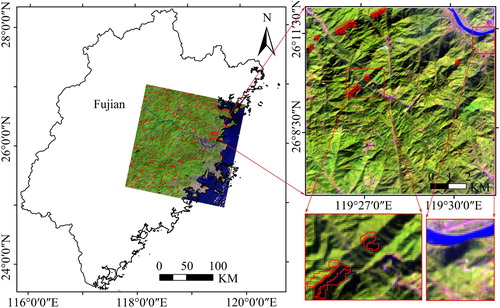
A Landsat8 Operational Land Imager (OLI) multispectral scene (119042), acquired on 13 December 2014 with a sun elevation of 36.85° and a sun azimuth of 155.27°, was downloaded and used in this study (left in Figure 1). Other reference data included ASTER GDEM V2 from the same site. The data sets were provided by Geospatial Data Cloud site, Computer Network Information Center, Chinese Academy of Sciences (http://www.gscloud.cn). The data pre-processing procedure also involved the calculation of top- of- atmosphere (TOA) reflectance of the whole image.

Figure 1. Research data, field survey location, subarea and validation samples.

2.2. Field survey area

In order to improve the study practicality, a field survey was conducted on 14 December 2015 in the area with geographical boundaries of 119°25′7″–119°31′27″E and 26°6′35″–26°12′15″N (top right in Figure 1). The surveyed mountainous region contains slopes ranging from 0° to 50° with an average of 23.44° and a standard deviation of 10.34°. It is also mainly covered by ecological forests with outstanding self and cast shadows and sunny slopes without shadow. So, a subarea with six main land-cover types, including water, cement roads, bare soil, vegetation in flat areas, vegetation on sunny slopes, vegetation on shady slopes, was selected for in-depth analysis (bottom right in Figure 1).

3. Methods

3.1. Conceptual model

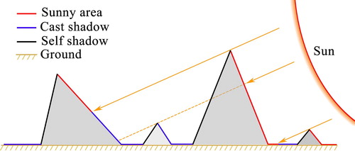
A common terrain shadow effect can result in the phenomena of ‘the same spectrum for different objects’ and ‘the same object with different spectra’ on the slopes oriented away from or towards the sun. Especially, the reflectance for vegetation retrieved from remote sensing images is decreased dramatically in terrain shadows, including the self shadow and cast shadow (Gilis 2001; Zhou et al. 2014; Li et al. 2016). In the context of a terrain radiative transfer model (Sandmeier and Itten 1997), the total pixel band irradiance in a rugged terrain includes direct solar irradiance, diffuse irradiance and adjacent terrain reflective irradiance. Diffuse irradiance is generally regarded as isotropic; therefore, their values are the same for slopes oriented both away from and towards the sun. However, the direct solar irradiance and adjacent terrain reflective irradiance are anisotropic (radiant directionality); therefore, their values distort for slopes of different orientations with respect to the sun and the adjacent terrain obstruction. Slopes oriented away from the sun become shady (shady slopes or self shadows) when their slope angle is larger than the sun elevation, while some slopes oriented towards the sun with higher mountains obstructed in the solar incidence direction also become shady (cast shadows) (Figure 2). In the perspective of topographic correction based on DEM, the band irradiance distortion in cast shadows cannot be eliminated but enlarged, because the irradiance on the slopes oriented towards the sun is always depressed according to the cosine of the solar incidence angle (cosi) (Li et al. 2016).

Figure 2. Schematic diagram of terrain shadows.

Accordingly, vegetation indices computed from these wavebands have some distortion (Δ_VI) with a reduction on terrain shadows, because the percentage change in the band total irradiance on the terrain shadows is different among spectral bands. Therefore, to eliminate terrain shadow effects, the vegetation index without terrain shadow effects can be modeled as:(1) ${\text{VI}}^{\mathrm{\prime }}=\text{VI}-{\mathrm{\Delta }}_{\mathrm{V}\mathrm{I}}$(1) where VI and VI′ are the vegetation index values with and without terrain shadow effects, respectively, and Δ_VI is the vegetation index value distortion resulting from terrain shadow effects.

An ideal vegetation index would be capable of rectifying this distortion by adding vegetation information on terrain shadow areas and suppressing vegetation information on sunny slopes without shadows while retaining vegetation information in flat surfaces. Suppose the ideal vegetation index named the shadow vegetation index (SVI) may rectify the distortion Δ_VI,(2) $\text{SVI}=-{\mathrm{\Delta }}_{\mathrm{V}\mathrm{I}},$(2) and a special conventional vegetation index (CVI) can be used to retrieve the information of VI′. Then a shadow eliminated vegetation index (SEVI) model that can eliminate terrain shadow effects would have the following form:(3) $\text{SEVI}=\text{CVI}+f(\mathrm{\Delta })\bullet \text{SVI},$(3) where f (Δ) is an adjustment factor to adjust the CVI and the corresponding SVI ratio to avoid under-elimination or over-elimination. Thus, the construction or selection of specific CVI and SVI become the first crucial step.

3.2. Band feature analysis

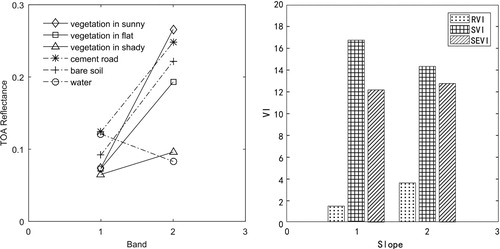
The sample data for the six land covers in the field survey area were selected manually on the image, and the average TOA reflectance values in red and near- infrared wavebands of every land cover sample were calculated and illustrated in Figure 3 (left). In the decreasing order of TOA reflectance values shown in Figure 3 (left), the red band exhibits the following trend: cement roads > water > bare soil > vegetation on sunny slopes >  vegetation in flat areas > vegetation on shady slopes; and the near-infrared band shows the following trend: vegetation on sunny slopes > cement roads > bare soil > vegetation in flat areas > vegetation on shady slopes > water. The TOA reflectance features of these two bands are different; however, they have the common property of exhibiting higher TOA reflectance values for vegetation on sunny slopes than those for vegetation on shady slopes. Moreover, the near-infrared TOA reflectance decreased more significantly from sunny slopes to shady slopes than that of the red waveband, which is the reason that conventional vegetation indices based only on simple band-ratio models cannot effectively eliminate terrain shadow effects.

Figure 3. TOA reflectance of six land-cover types (left) and VI values on shady and sunny slopes (right).

Note: bands #1–2 represent red and near-infrared wavebands, respectively (left); slopes #1–2 represent vegetation on shady slopes and sunny slopes without shadow, respectively (right).

3.3. Calculation and analysis of vegetation indices

The RVI is a simple, basic band-ratio index and a good indicator of LAI (Filella and Penuelas 1994), so it has the primary features of the proposed SEVI and becomes the first selection to construct SEVI. RVI is calculated as:(4) $\text{RVI}=\frac{B_{nir}}{B_r},$(4) where RVI is the ratio vegetation index, B_nir is the reflectance of the near-infrared band, and B_r is the reflectance of the red band.

In order to explain the vegetation index response to the terrain shadow effects, the points of vegetation on shady slopes and sunny slopes without shadows were analyzed (Figure 3 right). It is evident that the RVI of vegetation on shady slopes is much lower than that on sunny slopes without shadows because the reflectance of the near-infrared band decreases much more than that of the red band from the sunny slope without shadows to the shady slope (Figure 3 left).

Based on a detailed analysis of the reflectance of the red waveband, the most important finding is the inverse function of the red band reflectance, which represents the various land-cover features in the following order: vegetation on shady slopes > vegetation in flat areas > vegetation on sunny slopes > bare soil > water > cement roads. This inverse function of the red waveband amplifies the vegetation signal on shady slopes, so it is used to represent the shady vegetation index (SVI) that is calculated as:(5) $\text{SVI}=\frac{1}{B_r}.$(5)

The SVI value of vegetation on shady slopes is much higher than that on sunny slopes without shadow and complements the RVI (Figure 3 right). Meanwhile, it also conforms to the ideal SEVI model described in Equation 3. Therefore, the SEVI was constructed using RVI and SVI (Equation 6), both of which have a common denominator of the red waveband. Equation 6 meets the requirements of the conceptual SEVI in Equation 3.(6) $\text{SEVI}=\frac{B_{nir}}{B_r}+f\left(\mathrm{\Delta }\right)\bullet \frac{1}{B_r}.$(6)

3.4. Adjustment factor calculation model

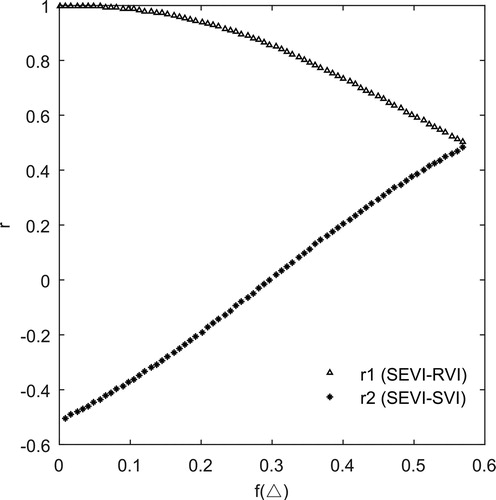
Most vegetation covers adjacent to shady and sunny slopes in rugged terrains are usually homogenous. Then, the mean vegetation information value of shady slopes is equal or similar to that of sunny slopes. Supposed that the ideal SEVI has the balanced linear correlations with the RVI and SVI respectively, an optimization algorithm for f (Δ) can be carried out as follows:

1. Calculate the correlation coefficient r₁ between SEVI and RVI (Equation 7) and r₂ between SEVI and SVI (Equation 8).(7) $r_1=\frac{n\sum x{y}_1-\sum x\bullet \sum y_1}{\sqrt{n{\sum x^2-\left(\sum x\right)}^2}\bullet \sqrt{n\sum y_1^2-{\left(\sum y_1\right)}^2}},$(7) (8) $r_2=\frac{n\sum x{y}_2-\sum x\bullet \sum y_2}{\sqrt{n{\sum x^2-\left(\sum x\right)}^2}\bullet \sqrt{n\sum {\text{y}}_2^2-{\left(\sum y_2\right)}^2}},$(8) where x is SEVI, y₁ is RVI, y₂ is SVI and n is the number of pixels in the subarea image.

2. Let f (Δ) vary from 0 to 1 with a fixed step of 0.001 and evaluate the difference between r₁ and r₂. When the difference between them reaches minimum (Equation 9), the optimized f (Δ) is determined.(9) $r_1-r_2\le \epsilon ,\epsilon \to 0,$(9)

Therefore, it is important to select the representative subarea, which meets the requirements for the determination of the optimized f (Δ). Combined with the field investigation and expert knowledge, the subarea with apparently rugged terrain and vegetation homogeneity was selected to calculate the suitable f (Δ) value (bottom middle in Figure 1). Finally, the optimized f (Δ) =  0.581 was adopted to calculate the SEVI for the research area (Figure 4).

Figure 4. Curves for f (Δ) optimization.

4. Validation

To validate the accuracy and effectiveness of SEVI in eliminating terrain shadow effects, three different methods were used, including the relative errors assessment of sample data, correlation analysis between VI and cosi, and contrast analysis of SEVI with conventional vegetation indices and correction models. Every set of sample data contained self shadows, cast shadows and adjacent sunny slopes without shadows in the whole scene. Three conventional vegetation indices were selected, including NDVI, RVI and EVI2, which are calculated with red and near-infrared reflectance and used extensively in vegetation parameters monitoring. The C topographic correction model and the atmospheric correction model of the second simulation of the satellite signal in the solar spectrum (6S) were introduced for contrast assessment. In practice, these three validation methods were jointly used.

4.1. Sample preparation

The three types of covers for self shadows, cast shadows and adjacent sunny slopes without shadows were selected according to the following computation methods.

1. Self shadows. A pixel is classified as a self shadow if its slope angle oriented away from the sun is greater than the sun elevation angle. So the triangular model was used to extract self shadows from the following equations:(10) $\tan \xi =\text{tan }\sigma \ast \cos (\pi -(\omega -\beta \left)\right)$(10) (11) $\tan \xi >\text{tan}\gamma$(11) where σ is the slope angle, β is the aspect angle, ω is the solar azimuth angle,γ is the sun elevation angle, and ξ is the slope angel oriented away from the sun. The values of σ and β were computed from DEM data, and the values of γ and ω were taken directly from the header files of the image.

2. Cast shadows. A shady pixel was labeled as a cast shadow when its slope angel is less than the sun elevation angle, regardless of the pixel aspect angle. So, the cast shadow samples were selected from the shadow area with slope angles less than 36.85°.

3. Sunny slopes without shadows. The sunny slopes without shadows, adjacent to the self and cast shadows, were chosen manually.

Finally, 532 sets of sample data including self shadows, cast shadows and sunny slope without shadows were selected from the whole image scene, based on the homogenous vegetation covers in every set of sample. Then the shape file of the 532 sets of samples was prepared to validate the SEVI performance in elimination of terrain shadow effects (red polygons in left of Figure 1).

4.2. Correction models

The conventional topographic correction models based on DEM include the Cosine, C, SCS (Sun-canopy-sensor) and SCS + C models (Teillet, Guindon, and Goodenough 1982; Gu and Gillespie 1998; Soenen, Peddle, and Coburn 2005). The C model, which takes into account the overcorrection of low illuminated slopes, is utilized widely (Riano et al. 2003), so it was adopted in this study. On the other hand, the 6S atmospheric correction physical model, as a good radiative transfer model, can accurately atmospherically correct an image’s digital numbers (Claverie et al. 2015). Therefore, the 6S model combined with a look-up table (Peng et al. 2016) was utilized to produce the comparable corrected surface reflectance for red and near infrared bands.

The C-model is calculated as:(12) $L_H=L_T\left(\frac{\cos \beta +c}{\cos i+c}\right),$(12) where L_H is the reflectance observed for a horizontal surface, L_T is the reflectance observed over an inclined surface, and c, which equals the quotient of the intercept b and the inclination a of the observed empirical linear correlation between L_T and cosi, is assumed to be constant for a given wavelength.

4.3. Conventional vegetation indices

The commonly used vegetation indices NDVI, RVI and EVI2 were used to represent the vegetation information of the research area. The NDVI is calculated as(13) $\text{NDVI}=\frac{B_{nir}-B_r}{B_{nir}+B_r}.$(13)

The EVI2 is calculated as(14) $\text{EVI2}=2.5\times \frac{B_{nir}-B_r}{B_{nir}+(6-7.5/2.08)\times B_r+1}.$(14)

The NDVI, RVI and EVI2 were computed from the original TOA reflectance and the corrected reflectance from the C and 6S + C models, while the SEVI was calculated directly from the TOA reflectance only.

5. Results

5.1. Comparison of vegetation indices

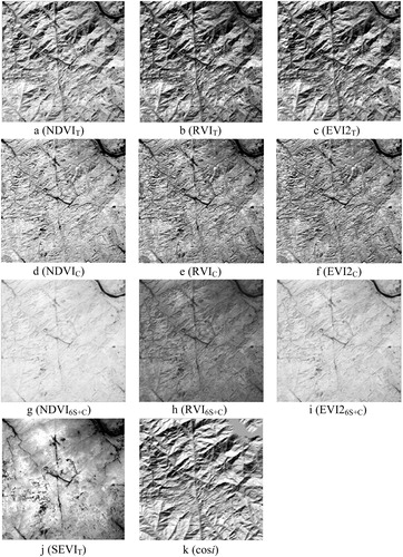
The three vegetation indices, NDVI, RVI and EVI2, and the proposed SEVI for the whole image were computed. Figure 5 shows these vegetation indices for the research area to better illustrate the effect in elimination of terrain shadows. The NDVI, RVI and EVI2 calculated from the TOA reflectance had strong a relief effect visually (Figure 5(a–c)), while the indices from the C corrected image achieved a better impression of relief reduction (Figure 5(d–f)). The NDVI, RVI and EVI2 computed from the 6S + C combined correction showed different relief effects for flat features (Figure 5(g–i)). Notably, the SEVI from TOA reflectance exhibited overall flat features, in which the impression of relief was drastically reduced and a high similarity with the NDVI from 6S + C corrected data was achieved (Figure 5(j and g)).

Figure 5. Vegetation indices in the research area.

Note: a–c, j represent vegetation indices computed from the TOA reflectance data, d–f represent vegetation indices computed from the C model corrected data, g–i represent vegetation indices computed from the 6S + C corrected data, and k represents cosi.

5.2. Validation via a comparison of self and cast shadows

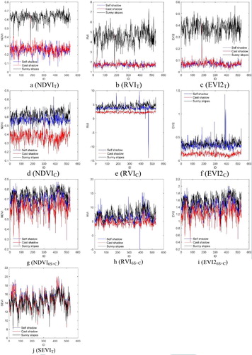
The plots of all the vegetation indices for the 532 sets of selected samples are shown in Figure 6. Clearly, the NDVI, RVI and EVI2 values in both self and cast shadows, which were directly calculated from TOA reflectance, were lower than those in sunny slopes (Figure 6(a–c)). After the C model topographic correction, these vegetation indices in self shadows were corrected and almost reached to the level in sunny slopes, while the vegetation indices in cast shadows were not corrected as much as in the self shadows (Figure 6(d–f)). Finally, after combined corrections of 6S model and C model, these vegetation indices both in self and cast shadows were obviously recovered and close to the level in sunny slopes, though the values for cast shadows were still a little low (Figure 6(g–i)). In contrast, the SEVI, calculated directly from the TOA reflectance, achieved almost the same result in elimination of terrain shadow effects in both self and cast shadows with very similar values in sunny slopes (Figure 6(j)).

Figure 6. Plots of vegetation indices for 532 sets of samples.

Note: a–c, j represent vegetation indices computed from the TOA reflectance data, d–f represent vegetation indices from the C model corrected data, and g–i represent vegetation indices from the 6S + C corrected data.

In order to further describe the elimination effect quantitatively in both self and cast shadows, the relative error (E) of corrected self shadow and cast shadow vegetation information was calculated. The relative error was computed as the following:(15) $\text{E}=|\text{V}{\text{I}}_{\mathrm{s}\mathrm{h}\mathrm{a}\mathrm{d}\mathrm{o}\mathrm{w}}-\text{V}{\text{I}}_{\mathrm{s}\mathrm{u}\mathrm{n}\mathrm{n}\mathrm{y}}|/\mathrm{V}{\text{I}}_{\mathrm{s}\mathrm{u}\mathrm{n}\mathrm{n}\mathrm{y}}\times 100\text{\%}.$(15) where VI_shadow is the vegetation indices in self shadow or cast shadow, VI_sunny is the vegetation indices in adjacent sunny slopes without shadows.

The relative error statistics are presented in Table 1. The relative errors of both self and cast shadows in NDVI, RVI and EVI2, computed from the TOA reflectance, were approximately equal to or greater than 60%, indicating that the terrain shadow effect is remarkable in the research area before any correction. After C model topographic correction, the relative errors of NDVI, RVI and EVI2 in self shadows declined to about 8.20%, 15.73% and 4.58%, respectively, but the relative errors in cast shadows were three times higher than those in self shadows, with respective values of 40.91%, 49.54% and 61.04%. These contrasting results validated the opinion that the topographic correction models based on DEM, such as the C model, lose their efficacy in cast shadows to a certain extent. As for the 6S + C combined corrected data, the NDVI achieved the lower relative errors both in self and cast shadows with about 6.52% and 18.01% respectively, whereas, the errors in cast shadows were still nearly three times higher than those in self shadows. The errors in cast shadows for RVI and EVI2 were relatively high with the values of 38.91% and 23.57%, respectively. These error values indicated that the accuracy of vegetation indices in elimination of cast shadows would improve when atmospheric correction was applied before topographic correction, but it was still lower than that in self shadows. In general, the traditional topographic corrections based on DEM inevitably lose their efficacy in elimination of cast shadows, even though it was combined with atmospheric correction. In comparison, the SEVI relative errors for both self and cast shadows were only 4.32% and 1.51%, respectively, which were much lower, especially for cast shadows, than those calculated from atmospheric and topographic corrected data.

Table 1. Mean (M) and relative error (E) of vegetation indices in self shadows, cast shadows and sunny slopes.

VI	Data	Mself	Mcast	Msunny	Eself (%)	Ecast (%)
NDVI	TOA	0.245	0.255	0.629	61.06	59.43
	C	0.568	0.366	0.619	8.20	40.91
	6S + C	0.695	0.610	0.744	6.52	18.01
RVI	TOA	1.667	1.708	4.526	63.16	62.26
	C	3.710	2.221	4.402	15.73	49.54
	6S + C	6.136	4.482	7.337	16.37	38.91
EVI2	TOA	0.064	0.070	0.374	83.01	81.40
	C	0.336	0.137	0.352	4.58	61.04
	6S + C	1.443	1.211	1.584	8.90	23.57
SEVI	TOA	14.744	14.348	14.134	4.32	1.51

5.3. Validation via a correlation analysis between cosi and VI

Correlation analysis between cosi and vegetation indices is a classic method to evaluate the elimination result of terrain shadow effects. The cosi is calculated as follows(16) $\cos i=\cos \sigma \ast \cos \theta +\sin \sigma \ast \sin \theta \ast \cos (\beta -\omega ),$(16) where i is the solar incidence angle, defined as the angle between the normal to the ground and the sun’s rays, σ is the slope angle, β is the aspect angle, θ is the solar zenith angle, and ω is the solar azimuth angle. The values of σ and β were computed from DEM data, and the values of θ and ω were taken directly from the header files of the image.

The 532 sets of cosi samples were calculated based on the sample shape file and cosi layer image. The scatter plots of cosi and vegetation indices are given in Figure 7, in which the points include the samples in self shadows (blue), cast shadows (red) and sunny slopes without shadows (black). From the scatter plots, the three types of samples were clearly separated. Firstly, the points in self shadows (blue) were separated by the line (cosi  =  0.0) from those in cast shadows and sunny slopes, indicating that the sample definitions of self shadows (Equation 10 and 11) and cast shadows are correct. Actually, the cast shadows are located in the flat area or the slopes shaded by the higher mountain (slope > sun elevation) in the solar incidence direction. Secondly, the linear regression analysis of samples showed that the NDVI, RVI and EVI2, calculated from the TOA reflectance, had high correlations with cosi, with coefficients of determination (r²) of 0.652, 0.642 and 0.691, respectively (Figure 7(a–c) and Table 2). Owing to the terrain shadow effects, the sample NDVI, RVI and EVI2 were dispersive with coefficients of variation (Std/Mean) of 48.20%, 52.97% and 87.58%, respectively. However, after C- model correction, the three types of sample points changed in vegetation index values with much more increasing in self shadows than in cast shadows and close to the values in sunny slopes without shadows (Figure 7(d–f) and Table 2). The linear correlations for the three vegetation indices changed from strong to weak with respective r² of 0.017, 0.035 and 0.001. The coefficients of variation of the three vegetation indices were reduced to 22.95%, 34.31% and 42.81%, respectively. As for the 6S + C combined corrections, the locations of the three types of points were further changed with values in cast shadows increased to the level of self shadows and sunny slopes (Figure 7(g–i) and Table 2). The linear relationships for NDVI, RVI and EVI2 were reduced with r² of 0.030, 0.033 and 0.033, respectively, while the coefficients of variation were changed to 12.80%, 33.82% and 17.12%, respectively. Finally, the SEVI values in the three types of samples were very similar with a r² of 0.032 with cosi and a coefficient of variation of 12.59% (Figure 7(j) and Table 2). It can be seen from these scatter plots and the coefficient of variation that the SEVI can achieve the same result as NDVI after 6S + C correction in elimination of topographic shadow effects.

Figure 7. Scatter plots of vegetation indices and cosi with 532 sets of samples.

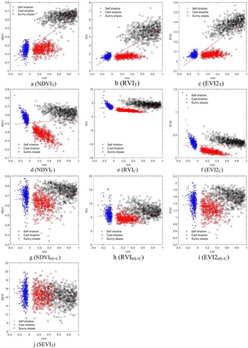
Table 2. Linear correlation analysis and coefficient of variation (Std/Mean) of 532 sets of samples.

VI	Data	r^2	k	d	Mean	Std	Std/Mean(%)
NDVI	TOA	0.652	0.438	0.254	0.380	0.183	48.20
	C	0.017	0.047	0.507	0.521	0.120	22.95
	6S + C	0.030	0.045	0.674	0.687	0.088	12.80
RVI	TOA	0.642	3.330	1.687	2.649	1.403	52.97
	C	0.035	0.659	3.284	3.474	1.192	34.31
	6S + C	0.033	1.097	5.722	6.039	2.042	33.82
EVI2	TOA	0.691	0.366	0.064	0.170	0.149	87.58
	C	0.001	0.008	0.274	0.276	0.118	42.81
	6S + C	0.033	0.131	1.385	1.423	0.244	17.12
SEVI	TOA	0.032	−0.960	14.770	14.490	1.825	12.59

Note: The r², k, and d are the coefficient of determination, line slope, and intercept, respectively.

6. Discussion

1. As a special vegetation index to remove terrain shadows effects, the SEVI achieved the accurate vegetation information by eliminating the effects from both self and cast shadows in rugged terrains with similar result from NDVI after 6S + C combined corrections. The SEVI was only calculated from the red and near-infrared wavebands without other heterogeneous data, while the 6S model and C model depend on the complicated atmospheric parameters and DEM data. Moreover, the DEM-based correction models, such as the C model, cannot achieve the satisfactory result in cast shadows as in self shadows. As for the improvement of SEVI, the combination model and the adjustment factor f (Δ) are two important aspects. The f (Δ) is the key and also the bottle neck to SEVI computation. The correlation coefficient-based algorithm presented in this paper is an empirical method and calculation accuracy depends on the terrain complexity and the proportion between the shadows and sunny slopes in the sample area. So the sample area for calculating f (Δ) is suggested to be selected from areas with high slopes and equal proportions between shadows and sunny slopes. The accuracy of the computed f (Δ) value also needs to be validated before its application in vegetation monitoring in large geographic regions. In the next step, a novel f (Δ) algorithm will be developed based on semi- physical or physical models and sun angles to calculate the global optimal value other than the local optimal value. On the other hand, the ratio and linear combinations are two basic forms of vegetation indices. The present SEVI combination model belongs to the linear combination form, so the CVI selection and SVI modification will be studied further. The ratio combination form can be evaluated in the development of the next version of SEVI.

2. The evaluation and selection of suitable vegetation indices is an important preprocessing step before the use of them in specific research targets and areas. Different vegetation indices have their own specific functions and features, including the advantages and disadvantages in retrieval of vegetation parameters in given cases. The SAVI and its serial improvements take effect in reduction of the soil background interference, while the ARVI and its variations are suitable for removal of atmospheric effects. The NDVI is a universal vegetation index and applied extensively, however, the saturation problem should be evaluated when it is used in high density vegetation areas. As for the application of vegetation indices in forests with rugged terrains, the accuracies in elimination of self and cast shadows effects should be firstly evaluated. Notably, the SEVI computed directly from the TOA reflectance is a good and simple solution. To sum up, the suitability and practicality of vegetation indices applied in rugged terrains should be assessed as a whole in the context of terrain shadow effect, saturation constraint, computation model complexity, input parameters, raw data accessibility and additional data error probability. Therefore, the SEVI is a novel option in retrieving vegetation information in rugged terrains within dense vegetation.

3. The systematic validation methods are important to assess the novel vegetation index in elimination of terrain shadow effects in rugged terrains. The correlation analysis between cosi and vegetation indices is the traditional and classic method to validate shadow elimination, but it is not robust enough. As the scatters plots shown in Figure 7, the NDVI, RVI and EVI2 calculated from C topographic corrected data had low coefficients of determination with cosi but they cannot practically remove the shadow effect in cast shadows. Therefore, the coefficient of variation of vegetation indices can be combined with the correlation analysis to evaluate the performance of vegetation indices in elimination of self and cast shadow effects. Only with low coefficient of variation of vegetation indices and coefficient of determination between cosi value and vegetation indices can the result be validated in elimination of topographic shadow effects in rugged terrains. In addition, the relative error assessment of sample data in self and cast shadows and adjacent sunny slopes without shadows, and comparison of conventional vegetation indices and correction models are also important validation methods. In practice, all three validation methods are recommended to be used to achieve reliable results.

4. The conventional topographic correction models based on DEM can easily lose their efficacy in cast shadows. The models, such as Cosine, C and SCS + C, are mainly based on the cosi, so the terrain shadow effect in self shadows are easily removed by these models, while the terrain shadow effect in cast shadows are difficult to eliminate. Actually, the vast majority of cast shadows are located in the flat area or the slopes oriented towards the sun but are shaded by the higher mountain (slope > sun elevation) in the solar incidence direction. The relative errors of NDVI, RVI and EVI2 in cast shadows, computed from the C model even combined with the 6S model, were validated several times higher than those in self shadows in this study (Table 1). Therefore, the lost efficacy in cast shadows of conventional DEM-based topographic correction models can’t be ignored. Accordingly, the elimination accuracy of the cast shadow effect should be considered in the development of better DEM-based topographic correction models in the future.

7. Conclusions

The exploration of vegetation indices is an important topic in remote sensing research. Although great progress has be made in the past half century, vegetation indices still have room for development to reduce the distortions as a result of sensor, solar, saturation, atmospheric and topographic effects. The proposed SEVI in this study was calculated from only red and near-infrared apparent reflectance without other heterogeneous data. It can produce accurate vegetation information with elimination of terrain shadow effects in both self and cast shadows. The SEVI is better than the conventional DEM-based topographic correction methods, such as the Cosine, C, SCS, SCS + C and 6S + C models, in removal of the terrain shadow effects, especially in cast shadows, and it also avoids additional errors from other heterogeneous data. The next step for future research will be to develop a better algorithm to determine f (Δ) based on the physical or semi-physical principles. The SEVI and future improved versions of it will also be applied to evaluate vegetation parameters in rugged terrains, such as the vegetation fraction, leaf area index, net primary productivity, and monitor ecological reservation change, and human disturbance.

Acknowledgements

This work was supported by the [China National Key Research and Development Plan] under Grant [2017YFB0504203]; [China Scholarship Fund] under Grant [201706655028]; and [Natural Science Foundation of Fujian Province, China] under Grant [2017J01658]. The authors thank two anonymous reviewers for their constructive suggestions and valuable comments.

Disclosure statement

No potential conflict of interest was reported by the authors.

ORCID

Hong Jiang http://orcid.org/0000-0002-1105-5205

Additional information

Funding

This work was supported by China National Key Research and Development Plan [grant number 2017YFB0504203]; China Scholarship Fund [grant number 201706655028]; Natural Science Foundation of Fujian Province [grant number 2017J01658].

References

- Bajocco, S., A. De Angelis, and L. Salvati. 2012. “A Satellite-based Green Index as a Proxy for Vegetation Cover Quality in a Mediterranean Region.” Ecological Indicators 23 (4): 578–587. doi:10.1016/j.ecolind.2012.05.013.
- Baret, F., and G. Guyot. 1991. “Potentials and Limits of Vegetation Indices for LAI and APAR Assessment.” Remote Sensing of Environment 35: 161–173. doi: 10.1016/0034-4257(91)90009-U
- Burgess, D., P. Lewis, and J. Muller. 1995. “Topographic Effects in AVHRR NDVI Data.” Remote Sensing of Environment 54: 223–232. doi: 10.1016/0034-4257(95)00155-7
- Claverie, M., E. Vermote, B. Franch, and J. Masek. 2015. “Evaluation of the Landsat-5 TM and Landsat-7 ETM+ Surface Reflectance Products.” Remote Sensing of Environment 169: 390–403. doi:10.1016/j.rse.2015.08.030.
- Colby, J. 1991. “Topographic Normalization in Rugged Terrain.” Photogrammetric Engineering and Remote Sensing 57: 531–537.
- Deng, Y., X. Chen, E. Chuvieco, T. Warner, and J. Wilson. 2007. “Multi-scale Linkages between Topographic Attributes and Vegetation Indices in a Mountainous Landscape.” Remote Sensing of Environment 111: 122–134. doi: 10.1016/j.rse.2007.03.016
- Fassnacht, F., H. Latifi, and B. Koch. 2012. “An Angular Vegetation Index for Imaging Spectroscopy Data-Preliminary Results on Forest Damage Detection in the Bavarian National Park, Germany.” International Journal of Applied Earth Observation and Geoinformation 19 (10): 308–321. doi: 10.1016/j.jag.2012.05.018
- Filella, I., and J. Penuelas. 1994. “The Red Edge Position and Shape as Indicators of Plant Chlorophyll Content Biomass and Hydric Status.” International Journal of Remote Sensing 15 (7): 1459–1470. doi: 10.1080/01431169408954177
- Gilabert, M., J. González-Piqueras, F. García-Haro, and J. Melia. 2002. “A Generalized Soil-adjusted Vegetation Index.” Remote Sensing of Environment 82: 303–310. doi: 10.1016/S0034-4257(02)00048-2
- Gilis, P. 2001. “Remote Sensing and Cast Shadow in Mountain Terrain.” Photogrammetric Engineering and Remote Sensing 67 (7): 833–839.
- Gitelson, A., Y. Kaufman, and M. Merzlyak. 1996. “Use of a Green Channel in Remote Sensing of Global Vegetation from EOS-MODIS.” Remote Sensing of Environment 58: 289–298. doi: 10.1016/S0034-4257(96)00072-7
- Gitelson, A., Y. Kaufman, R. Stark, and D. Rundquista. 2002. “Novel Algorithms for Remote Estimation of Vegetation Fraction.” Remote Sensing of Environment 80: 76–87. doi: 10.1016/S0034-4257(01)00289-9
- Gu, Y., J. Brown, J. Verdin, and B. Wardlow. 2007. “A Five-Year Analysis of MODIS NDVI and NDWI for Grassland Drought Assessment Over the Central Great Plains of the United States.” Geophysical Research Letters 34 (L06407): 6. doi:10.1029/2006GL029127.
- Gu, D., and A. Gillespie. 1998. “Topographic Normalization of Landsat TM Images of Forest Based on Subpixel Sun-Canopy-Sensor Geometry.” Remote Sensing of Environment 64 (2): 166–175. doi: 10.1016/S0034-4257(97)00177-6
- Gu, Y., B. Wylie, D. Howard, K. Phuyal, and L. Ji. 2013. “NDVI Saturation Adjustment: A New Approach for Improving Cropland Performance Estimates in the Greater Platte River Basin, USA.” Ecological Indicators 30: 1–6. doi:10.1016/j.ecolind.2013.01.041.
- Haboudane, D., J. R. Miller, N. Tremblay, P. J. Zarco-Tejada, and L. Dextraze. 2002. “Integrated Narrow Band Vegetation Indices for Prediction of Crop Chlorophyll Content for Application to Precision Agriculture.” Remote Sensing of Environment 81: 416–426. doi: 10.1016/S0034-4257(02)00018-4
- Holben, B., and C. Justice. 1981. “An Examination of Spectral Band Ratioing to Reduce the Topographic Effect on Remotely Sensed Data.” International Journal of Remote Sensing 2 (2): 115–133. doi: 10.1080/01431168108948349
- Huete, A. 1988. “A Soil-adjusted Vegetation Index (SAVI).” Remote Sensing of Environment 25: 295–309. doi: 10.1016/0034-4257(88)90106-X
- Huete, A., and H. Liu. 1994. “An Error and Sensitivity Analysis of the Atmospheric- and Soil-Correcting Variants of the NDVI for the MODIS- EOS.” IEEE Transactions on Geoscience and Remote Sensing 32: 897–905. doi: 10.1109/36.298018
- Jiang, Z., A. Huete, K. Didan, and T. Miura. 2008. “Development of a Two-band Enhanced Vegetation Index without a Blue Band.” Remote Sensing of Environment 112 (10): 3833–3845. doi:10.1016/j.rse.2008.06.006.
- Jiang, H., B. Wu, and X. Wang. 2010. “Developing a Novel Topography- Adjusted Vegetation Index (TAVI) for Rugged Area.” Proceedings of the 2010 IEEE International Geoscience and Remote Sensing Symposium (IGARSS 2010), 2075–2078. doi: 10.1109/IGARSS.2010.5654222
- Johansen, B., and H. Tommervik. 2014. “The Relationship between Phytomass, NDVI and Vegetation Communities Svalbard.” International Journal of Applied Earth Observation and Geoinformation 27: 20–30. doi:10.1016/j.jag.2013.07.001.
- Jordan, C. 1969. “Derivation of Leaf-area Index from Quality of Light on the Forest Floor.” Ecology 50: 663–666. doi:10.2307/1936256.
- Kaufman, Y., and D. Tanré. 1992. “Atmospherically Resistant Vegetation Index (ARVI) for EOS- MODIS.” IEEE Transactions on Geoscience and Remote Sensing 30: 261–270. doi: 10.1109/36.134076
- Li, H., L. Xu, H. Shen, and L. Zhang. 2016. “A General Variational Framework Considering Cast Shadows for the Topographic Correction of Remote Sensing Imagery.” ISPRS Journal of Photogrammetry and Remote Sensing 117: 161–171. doi:10.1016/j.isprsjprs.2016.03.021.
- Liao, Z., B. He, and X. Quan. 2015. “Modified Enhanced Vegetation Index for Reducing Topographic Effect.” Journal of Applied Remote Sensing 9 (096068): 1–21.
- Liu, F., Q. Qin, and Z. Zhan. 2012. “A Novel Dynamic Stretching Solution to Eliminate Saturation Effect in NDVI and Its Application in Drought Monitoring.” Chinese Geographical Science 22 (6): 683–694. doi: 10.1007/s11769-012-0574-5
- Matsushita, B., W. Yang, J. Chen, Y. Onda, and G. Qiu. 2007. “Sensitivity of the Enhanced Vegetation Index (EVI) and Normalized Difference Vegetation Index (NDVI) to Topographic Effects: A Case Study in High-density Cypress Forest.” Sensors 7 (11): 2636–2651. doi: 10.3390/s7112636
- Pei, F., C. Wu, X. Liu, X. Li, K. Yang, Y. Zhou, K. Wang, L. Xu, and G. Xia. 2018. “Monitoring the Vegetation Activity in China Using Vegetation Health Indices.” Agricultural and Forest Meteorology 248: 215–227. doi:10.1016/j.agrformet.2017.10.001.
- Peng, Y., G. He, Z. Zhang, T. Long, M. Wang, and S. Ling. 2016. “Study on Atmospheric Correction Approach of Landsat-8 Imageries Based on 6S Model and Look-up Table.” Journal of Applied Remote Sensing 10 (4): 045006. doi:10.1117/1.jrs.10.045006.
- Pinty, B., and M. Verstraete. 1992. “GEMI: A Non-linear Index to Monitor Global Vegetation from Satellites.” Vegetatio 101: 15–20. doi: 10.1007/BF00031911
- Propastin, P. 2009. “Spatial Non- Stationarity and Scale- Dependency of Prediction Accuracy in the Remote Estimation of LAI Over a Tropical Rainforest in Sulawesi, Indonesia.” Remote Sensing of Environment 113: 2234–2242. doi: 10.1016/j.rse.2009.06.007
- Qi, J., A. Chehbouni, A. Huete, Y. Kerr, and S. Sorooshian. 1994. “A Modified Soil- Adjusted Vegetation Index.” Remote Sensing of Environment 48: 119–126. doi: 10.1016/0034-4257(94)90134-1
- Qiu, B., Z. Wang, Z. Tang, Z. Liu, D. Lu, C. Chen, and N. Chen. 2016. “A Multi-scale Spatiotemporal Modeling Approach to Explore Vegetation Dynamics Patterns Under Global Climate Change.” GIScience and Remote Sensing 53 (5): 596–613. doi:10.1080/15481603.2016.1184741.
- Riano, D., E. Chuvieco, J. Salas, and I. Aguado. 2003. “Assessment of Different Topographic Corrections in Landsat-TM Data for Mapping Vegetation Types.” IEEE Transactions on Geoscience and Remote Sensing 41 (5): 1056–1061. doi: 10.1109/TGRS.2003.811693
- Rondeaux, G., M. Steven, and F. Baret. 1996. “Optimization of Soil-adjusted Vegetation Indices.” Remote Sensing of Environment 55: 95–107. doi: 10.1016/0034-4257(95)00186-7
- Rouse, J., R. Haas, J. Schell, and D. Deering. 1974. “Monitoring Vegetation Systems in the Great Plains with ERTS.” Third Earth Resources Technology Satellite-1 Symposium 1: 309–317, December 10, 1973, Washington, DC: NASA Scientific and Technical Information Office. https://ntrs.nasa.gov/search.jsp?R=19740022614.
- Sandmeier, S., and K. Itten. 1997. “A Physically-based Model to Correct Atmospheric and Illumination Effects in Optical Satellite Data of Rugged Terrain.” IEEE Transactions on Geoscience and Remote Sensing 35 (3): 708–717. doi: 10.1109/36.581991
- Soenen, S. A., D. R. Peddle, and C. A. Coburn. 2005. “SCS+C:A Modified Sun-Canopy-Sensor Topographic Correction in Forested Terrain.” IEEE Transactions on Geoscience & Remote Sensing 43 (9): 2148–2159. doi: 10.1109/TGRS.2005.852480
- Soudani, K., C. François, G. Le Maire, V. Le Dantec, and E. Dufrêne. 2006. “Comparative Analysis of IKONOS, SPOT, and ETM+ Data for Leaf Area Index Estimation in Temperate Coniferous and Deciduous Forest Stands.” Remote Sensing of Environment 102: 161–175. doi: 10.1016/j.rse.2006.02.004
- Teillet, P., B. Guindon, and D. Goodenough. 1982. “On the Slope-Aspect Correction of Multispectral Scanner Data.” Canadian Journal of Remote Sensing 8 (2): 84–106. doi: 10.1080/07038992.1982.10855028
- Tian, Q., Z. Luo, J. Chen, M. Chen, and F. Hui. 2007. “Retrieving Leaf Area Index for Coniferous Forest in Xingguo County, China with Landsat ETM+ Images.” Journal of Environmental Management 85: 624–627. doi: 10.1016/j.jenvman.2006.05.021
- Waring, R., N. Coops, W. Fan, and J. Nightingale. 2006. “MODIS Enhanced Vegetation Index Predicts Tree Species Richness across Forested Ecoregions in the Contiguous USA.” Remote Sensing of Environment 103 (2): 218–226. doi:10.1016/j.rse.2006.05.007.
- Xu, C., Y. Li, J. Hu, X. Yang, S. Sheng, and M. Liu. 2012. “Evaluating the Difference between the Normalized Difference Vegetation Index and Net Primary Productivity as the Indicators of Vegetation Vigor Assessment at Landscape Scale.” Environmental Monitoring and Assessment 184 (3): 1275–1286. doi:10.1007/s10661-011-2039-1.
- Yao, J., and Z. Zhang. 2006. “Hierarchical Shadow Detection for Color Aerial Images.” Computer Vision and Image Understanding 102 (1): 60–69. doi: 10.1016/j.cviu.2005.09.003
- Young, N., R. Anderson, S. Chignell, A. Vorster, R. Lawrence, and P. Evangelista. 2017. “A Survival Guide to Landsat Preprocessing.” Ecology 98 (4): 920–932. doi: 10.1002/ecy.1730
- Zhang, Z., G. He, X. Wang, and H. Jiang. 2011. “Leaf Area Index Estimation of Bamboo Forest in Fujian Province Based on IRS P6 LISS 3 Imagery.” International Journal of Remote Sensing 32 (19): 5365–5379. doi: 10.1080/01431161.2010.498454
- Zhou, Y., J. Chen, Q. Guo, R. Cao, and X. Zhu. 2014. “Restoration of Information Obscured by Mountainous Shadows through Landsat TM/ETM+ Images without the Use of DEM Data: A New Method.” IEEE Transactions on Geoscience and Remote Sensing 52 (1): 313–328. doi: 10.1109/TGRS.2013.2239651