Analysis of the dynamics of land use change and its prediction based on the integration of remotely sensed data and CA-Markov model, in the upstream Citarum Watershed, West Java, Indonesia

ABSTRACT

In this research, the integration of remotely sensed data and Cellular Automata-Markov model (CA-Markov) have been used to analyze the dynamics of land use change and its prediction for the next year. Training phase for the CA-Markov model has been created based on the input pair of land use, which is the result of land use mapping using Maximum Likelihood (ML) algorithm. Three-map comparison has been used to evaluate process accuracy assessment of the training phase for the CA-Markov model. Furthermore, the simulation phase for the CA-Markov model can be used to predict land use map for the next year. The analyze of the dynamics of land use change and its prediction during the period 1990 to 2050 can be obtained that the land serves as a water absorbent surfaces such as primary forest, secondary forest and the mixed garden area continued to decline. Meanwhile, on build land area that can lead to reduced surface water absorbing tends to increase from year to year. The results of this research can be used as input for the next research, which aims to determine the impact of land use changes in hydrological conditions against flooding in the research area.

KEYWORDS:

• Multi-temporal remotely sensed data
• CA-Markov model
• dynamics land use change

1. Introduction

A watershed is a spatial unit that has the form and the space required in hydrological studies. In addition, the hydrologic cycle also functions as a water flow system which flows from a high area to the lower area (Asdak 1995). The presence of imbalances in the watershed environment can lead to land degradation. One of the effects of environmental imbalances is the increasing runoff due to land use change in the watershed (Asdak 1995; Raharjo 2014). Land use is one of the important parameters that affect the increase of surface runoff (Kubal et al. 2009). In addition, there are also several other parameters such as vegetation cover, infiltration, evaporation, soil moisture, and several other interactions such as geology, slopes and climate processes (Newson 2002; Alexakis et al. 2014). Land use change is associated with increased flood events in the watershed environment, such as urbanization in water catchment areas leading to a decrease in water catchment zones. In the development of the current and future conditions of water resources are very sensitive to changes in land use and intensification of human activities. The risk of flooding will increase as a consequence of climate change on a local and global scale (Hadjimitsis et al. 2010; Alexakis et al. 2014).

The dynamics of land use changes can be monitored using remote sensing data. The availability of remote sensing data has provided a wide selection of variations of the resolution, namely: spectral, spatial, radiometric and temporal that can be used to detect changes in the Earth's surface (Li 2010; Lu et al. 2016; Yulianto et al. 2016). In addition, the utilization of remote sensing data can be used for extraction of land use information. Monitoring of land use change can be done by comparing the current multi-temporal conditions with the previous years (Behera et al. 2012; Halmy et al. 2015; Yulianto et al. 2016). The utilization of remote sensing data can be used to analyzing, monitoring and mapping land use changes (Treitz, Howard, and Gong 1992; Park, Chi, and Kwon 2003; Zope, Eldho, and Jothiprakash 2017). Remote sensing data has been carried out by several studies, such as: NOAA-AVHRR, MODIS, Landsat MSS, Landsat TM, Landsat ETM+, Landsat OLI/TIRS, ASTER, SPOT Vegetation, RapidEye and others (e.g. Lindgren 1985; Lanfredi et al. 2003; Tarantino, Blonda, and Pasquariello 2007; Al-Fares 2013; Adam et al. 2014; Owrangi, Lannigan, and Simonovic 2014; Yulianto et al. 2016; Hereher 2017).

Land use mapping is one of the important applications in remote sensing that can provide an overview of issues and trends topic studies and have a long history. Some of these studies have been developed significantly and including the development of classification algorithms, such as neural networks, decision tree, extreme learning machine, support vector machine, segmentation and object-based, sub-pixel-based, modified nearest neighbor classifier and others (e.g. Civco 1993; Pal and Mather 2003; Arslan 2009; Frohn et al. 2011; Lee and Lathrop 2011; Pal 2009, 2011). Ease of doing digital object classification has now simplified and performed by Luca, Michele, and Silvia (2013) by creating Semi-automatic Classification plugin tools in Quantum GIS software. The digital classification was developed based on supervised classification approach using maximum likelihood algorithm, which applies a Gaussian threshold value as a boundary class identified objects to the pixels of sampling pixels or training area. Some studies have applied this approach as was done by Huth et al. (2012); Portengen (2014); Yulianto et al. (2016).

Modeling and land use prediction have been developed with a variety of approaches and methods which are models of Markov Chain, Logistic regression, Cellular Automata and others (e.g. Muller and Middleton 1994; Mallinis and Koutsias 2008; Yang, Zheng, and Lv 2012; Hyandye, Mandara, and Safari 2015). Approach to modeling and land use prediction with the merger between the Cellular Automata and Markov Chain model (CA-Markov) is the most popular method and is often implemented by several studies up to now (e.g. Guan et al. 2011; Wang, Zheng, and Zang 2012; Yang, Zheng, and Chen 2014; Gong et al. 2015; Halmy et al. 2015). Markov Chain is a stochastic process model that can describe the change probabilities of the object to another object. The model is one of the recommended methods for land use modeling based on the time evolution trend (Thomas and Laurence 2006; Behera et al. 2012). Cellular Automata is one part of the essential elements of geospatial emphasis on variations of the changing dynamics of an event. In addition, the model can be used to simulate the characteristics of complex systems spatially and temporally (Mousivand, Sarab, and Shayan 2007; Arsanjani et al. 2013; Yang, Zheng, and Chen 2014).

The integration of remote sensing data and CA-Markov model can be used to create the prediction of future land use that is an important tool to evaluate and management of land use policies. In some studies, as has been done by Moiwo et al. (2010); Turnbull, Wainwright, and Brazier (2010) showed that the difference in the land use pattern of current conditions with previous years can be used as input in flood hydrological modeling. This is done in order to determine the hydrologic response to each scenario land use and amendments to the integrated approach which combined with spatial data and others.

Upstream Citarum Watershed is located in West Java province. That location has a large basin physiographic and better known as the Bandung basin and has a long history related to floods and various complex environmental problems (Muin, Boer, and Suharnoto 2015). The problems that the complex is not separated from the high pressure of population around Upstream Citarum. One manifestation of the pressure of the population is already causing land conversion around Upstream Citarum. Land use changes are the major problem with increasing the disappearance of undeveloped land and catchment area which may result in an increase in surface runoff, river flow during the rainy season and cause flooding. In addition, the deforestation also leads to an increase in landslides, erosion, and sedimentation as well as the decline in biodiversity (BAPPENAS 2013). Based on the background description and problems, the research questions are as follows: (a) How do the conditions of land use change in multi-temporal during the period from 1990 to 2016 in the research area? (b) How do the conditions of future land use for the next year based on change spatial pattern the period more than 20 years in the research area?.

The objectives of this research are (a) to create land use mapping and analysis of multi-temporal remote sensing data for the period 1990, 1996, 2000, 2003, 2009, and 2016. (b) to create the transition potential map based on the selection of variables physical factors that cause land use changes. (c) to create a trend-based modeling land use scenario or training phase for the CA-Markov model that looks out toward the year 2016 and establish land use basic scenario for the next future. (d) to create simulation phase for the CA-Markov model land use prediction in the next future based on the optimistic (best-conditions) and pessimistic (worst-conditions) scenarios.

2. Research area

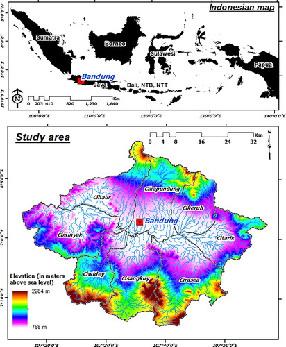
The research area is geographically located between 107⁰30′-108⁰00′E dan 6⁰43′-7⁰15′S. Upstream Citarum Watershed area covers several locations of regencies and cities located in the Province of West Java, namely: Bandung Regency, Cimahi City, Bandung City, and Sumedang City. The topography of the research area is a basin surrounded by the mountains of Tangkupan Perahu in the north, the Patuha-Malabar mountains in the south, the Krenceng mountains and the Mount of Mandalawangi in the west. Furthermore, it consists of seven sub-watersheds (Figure 1), namely: Citarik, Cirasta, Cisangkuy, Cikapundung, Ciwidey, Ciminyak, Cikeruh and Cihaur (Pratiwi 2011). Geological conditions in the research area by Silitongan (1973) and Bronto and Hartono (2006) can be divided into four categories, namely: (a) the old volcanic products with material made up of sand tuff, lapilli, and lava; (b) the young volcanic products with material made up of sand tuff, lapilli, lava and agglomerate material; (c) Tufa, pumice, consisting of sand tuff, lapilli, lava fragments of andesite-basalt; (d) The sand consists of sand tuffaceous material derived from the Mount of Tangkupan Perahu eruption.

Figure 1. The research area in the Upper Citarum watershed, West Java Province, Indonesia.

3. Data availability

In this research, remote sensing data were used to perform land use mapping and multi-temporal change analysis. Landsat data used in this study has the acquisition time in July and August (in the adjacent time) in each year, so the assumption that the data used had the same season every year. Landsat data, with a resolution of 30 m, at Level 1 Geometric (L1G) with sensor TM (path/row: 121/65 and 122/65) were used to input land use in 1990, 1996, 2003, and 2009. The ETM+ sensor was used to input land use in 2000, as well as sensors OIL/TIRS was used to input land use in 2016. Landsat 5 TM and SRTM30 DEM were provided by the US Geological Survey (USGS). Meanwhile, Landsat 7 ETM+, Landsat 8 OLI/TIR, and SPOT 6 were provided by Remote Sensing Technology and Data Center, LAPAN. In addition, the topographic map was provided by Geospatial Information Agency in Indonesian (BIG) are also used in this research as supporting data. The detail of spatial data types was used in this research can be shown in Table 1.

Table 1. Types of spatial data used in this study.

Data type	Path/row	Acquisition date	Spatial resolution / Map scale	Source
Landsat 5 TM	121/65;	03 August 1990;	30 m	USGS
	122/65	10 August 1990
Landsat 5 TM	121/65;	03 August 1996;	30 m	USGS
	122/65	25 July 1996
Landsat 7 ETM+	121/65;	22 August 2000;	30 m	LAPAN
	122/65	28 August 2000
Landsat 5 TM	121/65;	09 August 2003;	30 m	USGS
	122/65	16 August 2003
Landsat 5 TM	121/65;	07 August 2009;	30 m	USGS
	122/65	29 July 2009
Landsat 8 OLI / TIRS	121/65;	10 August 2016;	30 m	LAPAN
	122/65	17 August 2016
SPOT 6	–	Year 2016	1.5 m	LAPAN
SRTM30 DEM	–	11 February 2000	30 m	USGS
Topographic map	–	Year 1998	1:25,000	BIG

4. Methodology

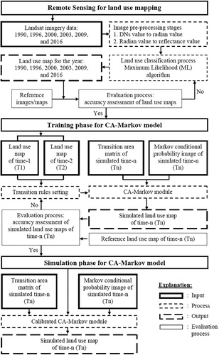
In general, the stages of this research method can be divided into three stages, namely (a) remote sensing for land use mapping, (b) training phase for CA-Markov model, and (c) simulation phase for the CA-Markov model. Flowchart of research can be shown in Figure 2.

Figure 2. Flowchart of the research.

4.1. Image pre-processing stages

The satellite image pre-processing stage was performed to convert the Digital Number (DNs) value to the reflectance value. In the standard products, Landsat 5 TM and Landsat 7 ETM+ have 8-bit unsigned integer format data. Meanwhile, the products Landsat 8 OLI/TIRS have 16-bit unsigned integer format data. Processing standard reflectance value needs to be done to address the differences in values format DNs on the satellite image. The conversion process DNs value to the reflectance values consists of two stages. The first stage of the conversion process is carried DNs value to the radians value. The second stage process is carried radian value to the reflectance values. Details on the second stage of the process refer to Chavez (1988), Luca, Michele, and Silvia (2013), USGS (2013a, 2013b).

4.2. Land use classification process and mapping

Land use classification process for mapping was applied to the Landsat and was based on Maximum Likelihood (ML) algorithm. This classification is a part of supervised classification methods that applying a Gaussian threshold limit value class of pixels. In addition, the methods have been identified at the time of sampling pixels and it was assumed that the probability distribution for each class of pixels is multivariate normal. In detail, the ML algorithm can be presented in Equations (1) and (2) (Richards and Jia 2006; Huang, Wang, and Budd 2009; Luca, Michele, and Silvia 2013; Yulianto et al. 2016). In this research, all the preprocessing stage Landsat imagery data, mapping, and land use classification process is done by using the Semi-Automatic Classification Plugin. The plugin is available in the open-source software on Quantum GIS (QGIS) 2.16.0 Nødebo that have been released since 22 July 2016 (http://www.qgis.org/id/site/). In addition, there are several reasons to use the Maximum Likelihood (ML) algorithm, i.e.: The ML algorithm is one of the most statistically established algorithms and uses the basis of probability calculations to view homogeneous objects and always display normal distributed histograms (Bayesian). The training area on the pixel is described as a specific object based on the shape, size and orientation of the sample on the feature space. In this classification, a pixel is assigned to a class according to its probability of belonging to a particular class. The ML algorithm uses a discriminate function to assign pixels to the class with the highest likelihood. Mean vector of each classes and covariance metrics are the key of ML algorithm as input of the discriminate factor that can be retrieved from training data and leads to gives the highest classification accuracy (Verrall 1991; Ahmad 2012; Hoglnd, Billor, and Anderson 2013). The research area is covered by not so many classes of the land use that we can identify of each class object. By considering these data, the mean of a certain class and the covariance can be obtained and we can assign the object to a certain class through classification methods for the classification of land use. Based on these points of views, the method of classification used in this research is the ML algorithm.(1) $G_i\left(x\right)=\ln p\left({\omega }_i\right)-\frac{1}{2}\ln \left|{\sum }_i\right|-\frac{1}{2}(x-m_i){\sum }_i^{-1}(x-m_i).$(1) Therefore:(2) $x\in {\omega }_i\text{if}{g}_i\left(x\right)>g_j\left(x\right)\text{for}\text{all}j\ne i,$(2) where $G_i\left(x\right)$ is the discriminant function in the ML algorithm. ${\omega }_i$ is the class, (where $i=1,\dots ,n$) and $M$ is the total number of classes. $x$ is a pixel in the $n$-dimensional vector, (where $n$ is the number of bands on the satellite image is used). $p\left({\omega }_i\right)$ is the true class opportunities, in ${\omega }_i$ for pixel positions $x$. $\left|{\sum }_i\right|$ is the decisive determinant of the covariance matrix of data in ${\omega }_i$ class. $\sum$ is the inverse covariance matrix of the data in ${\omega }_i$ class. $m_i$ is a vector average.

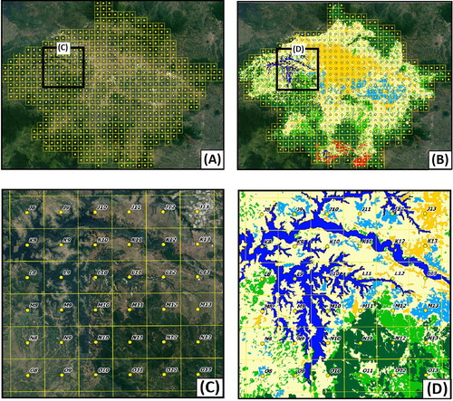
The evaluation process of accuracy assessment of the land uses classification were performed by error analysis matrix, as is done by Shooshtari and Gholamalifard (2015). In this research, making the Grid Index Feature (GIF) with a size of 2 km×2 km was used to determine the number of sample points in the accuracy assessment. In stratified sampling can be obtained a total of 650 points based center point of each polygon GIF. Example the validation and proportion training samples based on the making the GIF can be shown in Figure 3. In this research, the accuracy assessment land uses in 2003 and 2009 were based on the availability of high-resolution reference image from Google Earth, and land use in 2016 was based on the high-resolution reference image data SPOT 6 in 2016 obtained from LAPAN. Meanwhile, land use in the year 1990, 1996, and 2000 was not done the accuracy assessment due to unavailability of high-resolution data in these years. Accuracy assessment was done on each sample point GIF by comparing the land use classification results with the appearance of objects on the point of visual reference imagery interpretation, and then make an overall Kappa.

Figure 3. Example the validation and proportion training samples based on the making the Grid Index Feature (GIF) with a size of 2 km×2 km was used to determine the number of sample points in the calculation accuracy of assessment. In stratified sampling can be obtained a total of 650 points based center point of each polygon GIF. (A, C) SPOT 6 in 2016. (B,D) Land use map in 2016 based on the classification using Maximum Likelihood algorithm.

4.3. Training phase for CA-Markov model

Analysis of the dynamics of land use change in 1990 to 2016 can be done with a broad view and compare the changes and percentage. This is done in each class land use which has been derived based on data from Landsat imagery in 1990, 1996, 2000, 2003, 2009 and 2016. Land uses data were used as input data pairs during time-1 and time-2, and 10 combinations of data inputs are performed as a training phase for the CA-Markov model to obtain an evaluation of the pairs data in simulated land use in 2016. The results of the classification land use map in the year 2016 were used as a base reference (reference land use map of time in 2016) to create simulated future land use. There are 10 combinations of data inputs (land use map of time-1 (T1) and land use map of time-2 (T2)) to simulated future land use in time-n (Tn), namely: input for time-1 in 1990 & time-2 in 1996; input for time-1 in 1990 & time-2 in 2000; input for time-1 in 1990 & time-2 in 2003; input for time-1 in 1990 & time-2 in 2009; input for time-1 in 1996 & time-2 in 2000; input for time-1 in 1996 & time-2 in 2003; input for time-1 in 1996 & time-2 in 2009; input for time-1 in 2000 & time-2 in 2003; input for time-1 in 2000 & time-2 in 2009; and input for time-1 in 2003 & time-2 in 2009. In this research, land use modeling and prediction are based on the CA-Markov model. According to Thomas and Laurence (2006), Behera et al. (2012), Yang, Zheng, and Chen (2014), CA-Markov is a model that combines Markov Chain and Cellular Automata approaches that can be used to land uses predict for the next year. Furthermore, modeling and land use prediction can be done by using the tools CA-Markov software IDRISI Andes, which was developed by the Lab. Clark at Clark University.

There are three steps being taken to implement the CA-Markov model for simulated land use, namely: (a) calculate the transition area matrix of land use in simulated time-n, (b) calculate Markov conditional probability image of simulated time-n, (c) create a map of potential transition rules setting, and (c) simulated land use map of time-n. In the first stage, the transition matrix calculations performed to generate probabilities area the possibility of a change in a land uses class become more land use class within a certain time period, which can be served by Equation (3). In addition, the calculation on that analysis also generates probabilities transition matrix which is the probability of each pixel of the land use class to turn into other land use class. The calculation can be presented in Equation (4). The accuracy of the results of the estimation matrix transition area and transition probability matrix is determined based on the value of the error probabilities are 15% (Yang, Zheng, and Chen 2014).(3) $P_{\left(N\right)}=P_{(N-1)}xP,$(3) where P is the probabilities transition matrix on land use types derived from two different years on land use map. ${\text{P}}_{\left(\mathrm{N}\right)}$ is a state opportunity during or predictions of the near future (probability of any state times). ${\text{P}}_{(\mathrm{N}-1)}$ is the initial state opportunities (preliminary state probability).(4) $A=\left[\begin{array}{c}{A}_{11}\\ A_{21}\\ .\\ .\\ .\\ A_{n1}\end{array}\begin{array}{c}{A}_{12}\\ A_{22}\\ .\\ .\\ .\\ A_{n2}\end{array}\begin{array}{c}\dots \\ \dots \\ .\\ .\\ .\\ \dots \end{array}\begin{array}{c}{A}_{1n}\\ A_{2n}\\ .\\ .\\ .\\ A_{nn}\end{array}\right],$(4) where A is the transition matrix area. $A_{ij}$ is the total area of land use class i to class j for year prediction from the starting point to the target of the simulation period. n is the number of land use types.

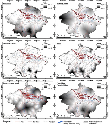
In the second stage, transition potential map simulation on the basis of a CA-Markov model, which is used as a controlling factor land use spatial distribution. Map of potential transition at earlier stage opportunities created by the transition matrix. At this stage, the potential map for the transition made land use class that will experience a change or transit to other land use class have the same opportunities. In this research, the physical parameters in making the transition potential map, include elevation, distance from the primary road, distance from the secondary road, distance from the river, and distance from other water sources (such as lakes and reservoirs). In stage three, do predictive simulation land use (Thomas and Laurence 2006; Behera et al. 2012; Arsanjani et al. 2013). At this stage, the process can be carried out within the framework of the spatial CA-Markov module that can be presented in Equation (5). The process takes time iteration, the integration of the transition matrix area, the map of potential transition, and land use be simulated at some time in the next future (Yang, Zheng, and Chen 2014).(5) $\text{if}{S}_j=max(S_1,S_2,\dots ,S_n)\text{and}\text{Are}{\text{a}}_{ij}<\frac{A_{ij}}{T}\text{then}{C}_i\to C_j,$(5)

where $S_j$ is a class of potential land use which will transit to land use class j. $Are{a}_{ij}$ is the total area of land use from land use class i to class j in the iteration process. $T$ is the iteration time.

4.4. The evaluation process for accuracy assessment simulated land use maps

The evaluation of the results of the training phase for the CA-Markov model was performed by a three-map comparison method as proposed by Pontius et al. (2008). This method is a validation technique by applying overlay three maps: the reference map of time-1, the reference map of time-2, and the simulated map for time-2. Three-map comparison approach can show a comparison between the correct pixels due to persistence and correct pixels due to change observed. This evaluation method proved to be more suitably applied to the results of land use simulated, when compared to the Kappa calculation method (Pontius and Millones 2011; Paegelow et al. 2014, 2018). Kappa values tend to experience inflation and are less able to explain whether the accuracy value obtained is due to an accurate prediction of change, or no change, or change according to the predicted class (Pontius et al. 2008; Pontius and Millones 2011; van Vliet, Bregt, and Hagen-zanker 2011; Ahmed, Ahmed, and Zhu 2013; van Vliet et al. 2016). Three-map comparison will divide the model evaluation results into four components, namely: A is the error due to observed change predicted as persistence. B is the Correct due to observed change predicted as change. C is the error due to observed change predicted as wrong gaining category. D is the error due to observed persistence predicted as change. Furthermore, these four components are used to calculate model errors, which consist of figure of merit, producer's accuracy, and user's accuracy in percent (Pontius et al. 2008).

4.5. Simulation phase for CA-Markov model

In this research, the simulation phase for the CA-Markov model can be predicted based on the optimistic (best-conditions) and pessimistic (worst-conditions) scenarios. The input land uses data refers to the results of the evaluation process accuracy assessment using the three-map comparison method. Furthermore, based on the results of the evaluation process, the future land use can be simulated in 2025 to 2050 with optimistic and pessimistic scenarios.

5. Results

5.1. Land use classification and mapping

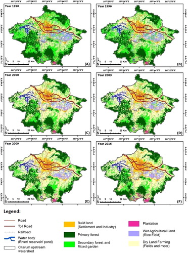
This research has been produced multi-temporal land use maps in 1990 to 2016 that have been classified by the ML algorithm. Land use classification and mapping was generated from input Landsat images could be obtained six class land uses, namely: ‘build land (settlement and industry)’, ‘primary forest’, ‘secondary forest and mixed garden’, ‘plantation’, ‘wet agricultural land (rice field)’, and ‘dry land farming (fields and moor)’. The result of accuracy assessment land use classification is based on the error matrix, which is stratified sampling a total of 650 points can be obtained from the manufacturing center point on a GIF with the size of 2 km×2 km. Accuracy assessment of land use in 2003 and 2009 ware based on the reference high-resolution imagery from Google Earth in 2003 and 2009. Meanwhile, land use in 2016 based on the high-resolution reference SPOT 6 image in 2016. Land use in 1990, 1996, and 2000 are not the accuracy assessment due to unavailability of high-resolution data in the research area. The results of accuracy assessment of land use maps in 2003, 2009, and 2016 are 85.7%, 84.4% and 88.2%, respectively. The results of multi-temporal land use mapping in 1990 to 2016 can be shown in Figure 4.

Figure 4. The results of multi-temporal land use mapping in 1990 to 2016 based on the supervised classification using the ML algorithm. (A) 1990, (B) 1996, (C) 2000, (D) 2003, (E) 2009, (F) 2016.

5.2. Analyze of the dynamics land use changes

Based on the results of land use mapping in 1990, 1996, 2000, 2003, 2009 and 2016, the percentage area of the dynamics land use changes in 1990 to 2016 can be shown in Table 2. Meanwhile, the estimate of average area land use changes in 1990 to 2016 can be shown in Table 3. For land use class ‘build land’ to keep extending widely from the year 1990 to 2016, with an increase in the average area of 437.5 ha/year. For land use class ‘primary forest’ area tends to decrease from the year 1990 to 2016, with average area decreased by 488.6 ha/year. In the class of ‘secondary forest and mixed garden’ are likely to continue to decline comprehensive in the year 1990 to 2016, with average area decreased by 1231.5 ha/year. In the class ‘dry land farming’ to keep extending widely from the year 1990 to 2016, the average area increased by 1373.7 ha/year. In the class of ‘plantation’ to keep extending widely from year 1990 to 2016, the average area increased by 119.1 ha/year. In the class ‘water body’ average area tends to be stable. Meanwhile, the ‘wet agriculture land’ area continued to decline from the year 1990 to 2016, with average area decreased by 210.2 ha/year.

Table 2. The percentage area of the dynamics land use changes in 1990 to 2016.

Land use	Year
	1990		1996		2000		2003		2009		2016
	Area (ha)^a		Area (ha)^a		Area (ha)^a		Area (ha)^a		Area (ha)^a		Area (ha)^a
Build land (Settlement and Industry)	16329	(7.1)	17740	(7.8)+	18,835	(8.2)+	19,957	(8.7)+	22,488	(9.8)+	27,703	(12.1)+
Primary forest	66,185	(29.0)	61,447	(26.9)−	58,933	(25.8)−	58,144	(25.4)−	54,548	(23.9)−	53,481	(23.4)−
Secondary forest and mixed garden	60,436	(26.4)	53,412	(23.4)−	32,556	(14.2)−	32,154	(14.1)−	31,487	(13.8)−	28,418	(12.4)−
Dry land farming (Fields and moor)	64,464	(28.2)	77,410	(33.9)+	100,871	(44.1)+	101,129	(44.3)+	103,068	(45.1)+	100,180	(43.8)−
Plantation	1953	(0.9)	2203	(1.0)+	2377	(1.0)+	2518	(1.1)+	3049	(1.3)+	5050	(2.2)+
Water body (River/reservoir/pond)	3858	(1.7)	3857	(1.7)−	3858	(1.7)+	3833	(1.7)−	3837	(1.7)+	3859	(1.7)+
Wet agriculture land (Rice field)	15,294	(6.7)	12,450	(5.4)−	11,089	(4.9)−	10,784	(4.7)−	10,042	(4.4)−	9828	(4.3)−
Total	228,519	(100)	228,519	(100)	228,519	(100)	228,519	(100)	228,519	(100)	228,519	(100)

^aPercentage area, ‘−’ decrease; ‘+’ increase.

Table 3. The estimate of average area land use changes in 1990 to 2016.

Land use	Change area (Ha)					Average area (ha/year)
	1990 to 1996	1996 to 2000	2000 to 2003	2003 to 2009	2009 to 2016
Build land (Settlement and Industry)	+1411	+1095	+1122	+2531	+5215	+437.5
Primary forest	−4738	−2514	−789	−3596	−1067	−488.6
Secondary forest and mixed garden	−7024	−20856	−402	−667	−3069	−1231.5
Dry land farming (Fields and moor)	+12,946	+23461	+258	+1939	−2888	+1373.7
Plantation	+250	+174	+141	+531	+2001	+119.1
Water body (River/reservoir/pond)	0	+1	−25	+4	+22	0.0
Wet agriculture land (Rice field)	−2844	−1361	−305	−742	−214	−210.2

Note: ‘−’ decrease; ‘+’ increase.

5.3. Training phase for CA-Markov model

The results of remote sensing for land use mapping in 1990 to 2016 were used as inputs to create simulated land use map of time-n using the CA-Markov model. In addition, several other inputs, such as elevation, distance to primary roads, distance to secondary roads, distance to the river, and distance to other water sources were used as parameters to create a potential transition map (transition rules setting). The results of potential transition map in the research area can be presented in Figure 5, which can show as an indicator of physical factors that can affect land use changes in the research area.

Figure 5. Inputs and parameters to create a transition potential map (A) elevation. (B) Distance from the primary road. (C) Distance from the secondary road. (D) Distance from the river. (E) Distance from reservoir and pond. (F) Result of transition potential map.

In this research, land use map in 2016 was used as controls simulated future land use of time-n (Tn) and used to reference land use map for evaluation process training phase for the CA-Markov model. There are 10 combinations of data inputs (land use map of time-1 (T1) and land use map of time-2 (T2)) to simulated future land use in time-n (In this case, Tn = in year 2016). The results of simulated land use in time-n or Tn = in year 2016 based on the 10 combinations of input data land use can be presented in Figures 6 and 7. The accuracy assessment of simulated land use maps in training phase for the CA-Markov model can be evaluated with the method of three-comparison maps. The result of validation maps using three-map comparison obtained by overlaying the reference map of time 1, the reference map of time 2, and the prediction map for time 2 can be shown in Table 4 and Figure 8. Based on the result of validation maps using three-map comparison can be obtained that the three pairs of data with the highest accuracy are reference map of time 1 (in 2000), reference map of time 2 (in 2016), and simulated map for time 2 (in 2016 for pairs input data in 2000 & 2009). The percentage values for figure of merit, producer's accuracy, and user's accuracy are 72.5%, 78.5% and 79.6%, respectively. Meanwhile, three pairs of data with the lowest accuracy are reference map of time 1 (in 1990), reference map of time 2 (in 2016), and simulated map for time 2 (in 2016 for pairs input data in 1990 & 1996). The percentage values for figure of merit, producer's accuracy, and user's accuracy are 50.7%, 57.3% and 56.4%, respectively.

Figure 6. (A) Land use simulated in 2016 using input data from the year 1990 and 1996. (B) Land use simulated in 2016 using input data from the year 1990 and 2000. (C) Land use simulated in 2016 using input data from the year 1990 and 2003. (D) Land use simulated in 2016 using input data from the year 1990 and 2009. (E) Land use simulated in 2016 using input data from the year 1996 and 2000.

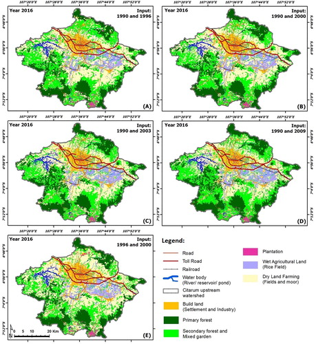
Figure 7. (A) Land use simulated in 2016 using input data from the year 1996 and 2003. (B) Land use simulated in 2016 using input data from the year 1996 and 2009. (C) Land use simulated in 2016 using input data from the year 2000 and 2009. (D) Land use simulated in 2016 using input data from the year 2000 and 2009. (E) Land use simulated in 2016 using input data from the year 2003 and 2009.

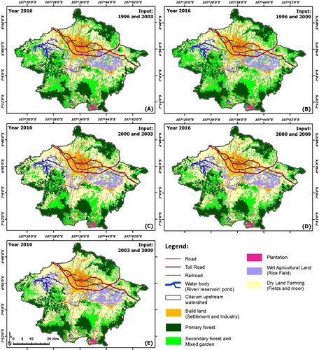
Figure 8. The result of validation maps using three-map comparison obtained by overlaying the reference map of time 1, the reference map of time 2, and the prediction map for time 2.

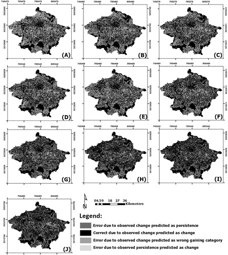
Table 4. The results of calculation accuracy assessment or validation maps using three-map comparison obtained by overlaying the reference map of time 1, the reference map of time 2, and the prediction map for time 2.

ID	Reference of time 1	Reference of time 2	Prediction map for time 2	Figure of merit	Producer's accuracy	User's accuracy	Information
A	1990	2016	2016: (input 1990 & 1996)	50.7	57.3	56.4	Pessimistic scenario
B	1990	2016	2016: (input 1990 & 2000)	54.1	58.8	61.6	–
C	1990	2016	2016: (input 1990 & 2003)	55.7	59.5	63.6	–
D	1990	2016	2016: (input 1990 & 2009)	56.1	59.7	63.8	–
E	1996	2016	2016: (input 1996 & 2000)	56.7	64.5	62.4	–
F	1996	2016	2016: (input 1996 & 2003)	61.0	66.1	67.9	–
G	1996	2016	2016: (input 1996 & 2009)	63.1	66.9	71.4	–
H	2000	2016	2016: (input 2000 & 2003)	71.8	78.3	76.2	–
I	2000	2016	2016: (input 2000 & 2009)	72.5	78.5	79.6	Optimistic scenario
J	2003	2016	2016: (input 2003 & 2009)	70.8	75.1	78.1	–

5.4. Simulation phase for CA-Markov model

Furthermore, a pair of input data which will be used to simulate future land use in 2025, 2030, 2035, 2040, 2045 and 2050 are selected based on the calculation results of accuracy assessment using three-map comparison. Land use data pairs in 2000 and 2009 with results of three-map comparison for reference map of time 1 (in 2000), reference map of time 2 (in 2016), and simulated map for time 2 (in 2016 for pairs input data in 2000 & 2009) were used to create simulated future land use with the optimistic scenario (best-conditions) and the results of future land use simulated in 2025 to 2050 can be presented in Figure 9. Meanwhile, land use data pairs in 1990 and 1996 with results of three-map comparison for reference map of time 1 (in 1990), reference map of time 2 (in 2016), and simulated for time 2 (in 2016 for pairs input data in 1990 & 1996) were used to create simulated future land use with the conditions of worst or pessimistic scenario and the results of future land use simulated in 2025 to 2050 can be presented in Figure 10. The results of future land use change area in 2025 to 2050 for the optimistic scenario and the estimated change of average area can be shown in Tables 5 and 6. In the class ‘build land’ is generally expected to continue to increase during the period 2025 to 2050 is based on the values of optimistic scenario, with the average area of 323.7 ha/year. In the class of ‘primary forest’ is expected to continue to decline with the average area of 225 ha/year. In the class of ‘secondary forest and mixed garden’ is expected to continue to decline with the average area of 151 ha/year. In the class ‘dry land farming’ is expected to continue to increase with the average area of 3.2 ha/year. In the class of ‘plantation’ is expected to increase with the average area of 69.8 ha/year. In the class ‘water body’ tends to be relatively stable with the average area of 0.1 ha/year. Meanwhile, in the class of ‘wet agriculture land’ is estimated to decrease by average area of 20.8 ha/year.

Figure 9. Future land use simulated in 2025 to 2050 for optimistic scenarios with the percentage values for figure of merit, producer's accuracy, and user's accuracy are 72.5%, 78.5% and 79.6%, respectively.

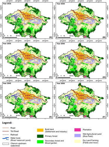
Figure 10. Future land use simulated in 2025 to 2050 for pessimistic scenarios with the percentage values for figure of merit, producer's accuracy, and user's accuracy are 50.7%, 57.3% and 56.4%, respectively.

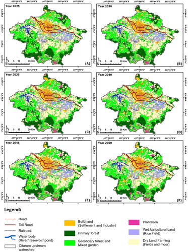
The results of future land use change area in 2025 to 2050 for the pessimistic scenario and the estimated change of average area can be presented in Tables 7 and 8. Based on the pessimistic scenario the value land use change predictions in 2025 to 2050 for the class of ‘build land’, ‘secondary forest and mixed garden’, ‘dry land farming’, ‘plantation’, and ‘wet agriculture land’ is expected to continue to increase, with average an area of 173.7 ha/year, 3.4 ha/year, 155.5 ha/year, 37 ha/year, and 19.2 ha/year, respectively. Meanwhile, the ‘primary forest’ and ’water body’ is expected to decline, with the average area of 388.6 ha/year and 0.2 ha/year, respectively.

Table 5. Future land use simulated change area in 2025 to 2050 for optimistic scenarios with the percentage values for figure of merit, producer's accuracy, and user's accuracy are 72.5%, 78.5% and 79.6%, respectively.

Land use	Year
	2025		2030		2035		2040		2045		2050
	Area (ha)^a		Area (ha)^a		Area (ha)^a		Area (ha)^a		Area (ha)^a		Area (ha)^a
Build land (Settlement and Industry)	25,082	(11.0)	26,902	(11.8)+	28,659	(12.5)+	30,269	(13.2)+	31,779	(13.9)+	33,175	(14.5)+
Primary forest	47,016	(20.6)	45,716	(20.0)−	44,558	(19.5)−	43,429	(19.0)−	42,390	(18.5)−	41,391	(18.1)−
Secondary forest and mixed garden	38,302	(16.8)	37,406	(16.4)−	36,504	(16.0)−	35,793	(15.7)−	35,116	(15.4)−	34,527	(15.1)−
Dry land farming (Fields and moor)	98,995	(43.3)	99,136	(43.4)+	99,175	(43.4)+	99,178	(43.4)+	99,138	(43.4)−	99,074	(43.4)−
Plantation	3389	(1.5)	3756	(1.6)+	4127	(1.8)+	4469	(2.0)+	4810	(2.1)+	5133	(2.2)+
Water body (River/reservoir/pond)	3279	(1.4)	3280	(1.4)+	3282	(1.4)+	3272	(1.4)−	3275	(1.4)+	3282	(1.4)+
Wet agriculture land (Rice field)	12,457	(5.5)	12,323	(5.4)−	12,214	(5.3)−	12,110	(5.3)−	12,012	(5.3)−	11,937	(5.2)−
Total	228,519	(100)	228,519	(100)	228,519	(100)	228,519	(100)	228,519	(100)	228,519	(100)

^aPercentage area, ‘−’ decrease; ‘+’ increase.

Table 6. The estimate of average area of the future land use simulated in 2025 to 2050 for optimistic scenarios with the percentage values for figure of merit, producer's accuracy, and user's accuracy are 72.5%, 78.5% and 79.6%, respectively.

Land use	Change area (Ha)					Average area (ha/year)
	2025 to 2030	2030 to 2035	2035 to 2040	2040 to 2045	2045 to 2050
Build land (Settlement and Industry)	+1820	+1757	+1610	+1510	+1396	+323.7
Primary forest	−1300	−1158	−1129	−1039	−999	−225.0
Secondary forest and mixed garden	−896	−902	−711	−677	−589	−151.0
Dry land farming (Fields and moor)	+141	+39	+3	−40	−64	+3.2
Plantation	+367	+371	+342	+341	+323	+69.8
Water body (River/reservoir/pond)	+1	+2	−10	+3	+7	+0.1
Wet agriculture land (Rice field)	−134	−109	−104	−98	−75	−20.8

Note: ‘−’ decrease; ‘+’ increase.

Table 7. Future land use simulated change area in 2025 to 2050 for pessimistic scenarios with the percentage values for figure of merit, producer's accuracy, and user's accuracy are 50.7%, 57.3% and 56.4%, respectively.

Land use	Year
	2025		2030		2035		2040		2045		2050
	Area (ha)^a		Area (ha)^a		Area (ha)^a		Area (ha)^a		Area (ha)^a		Area (ha)^a
Build land (Settlement and Industry)	24060	(10.5)	25151	(11.0)+	26105	(11.4)+	26962	(11.8)+	27729	(12.1)+	28402	(12.4)+
Primary forest	41307	(18.1)	39120	(17.1)−	37056	(16.2)−	35119	(15.4)−	33300	(14.6)−	31592	(13.8)−
Secondary forest and mixed garden	64787	(28.4)	64723	(28.3)−	64708	(28.3)−	64733	(28.3)+	64793	(28.4)+	64873	(28.4)+
Dry land farming (Fields and moor)	77486	(33.9)	78366	(34.3)+	79189	(34.7)+	79964	(35.0)+	80689	(35.3)+	81373	(35.6)+
Plantation	3015	(1.3)	3198	(1.4)+	3385	(1.5)+	3577	(1.6)+	3761	(1.6)+	3941	(1.7)+
Water body (River/reservoir/pond)	3277	(1.4)	3268	(1.4)−	3287	(1.4)+	3286	(1.4)−	3274	(1.4)−	3273	(1.4)−
Wet agriculture land (Rice field)	14587	(6.4)	14692	(6.4)+	14789	(6.5)+	14879	(6.5)+	14973	(6.6)+	15066	(6.6)+
Total	228519	(100)	228519	(100)	228519	(100)	228519	(100)	228519	(100)	228519	(100)

^aPercentage area, ‘−’ decrease; ‘+’ increase.

Table 8. The estimate of average area of the future land use simulated in 2025 to 2050 for pessimistic scenarios with the percentage values for figure of merit, producer's accuracy, and user's accuracy are 50.7%, 57.3% and 56.4%, respectively.

Land use	Change area (Ha)					Average area (ha/year)
	2025 to 2030	2030 to 2035	2035 to 2040	2040 to 2045	2045 to 2050
Build land (Settlement and Industry)	+1091	+954	+857	+767	+673	+173.7
Primary forest	−2187	−2064	−1937	−1819	−1708	−388.6
Secondary forest and mixed garden	−64	−15	+25	+60	+80	+3.4
Dry land farming (Fields and moor)	+880	+823	+775	+725	+684	+155.5
Plantation	+183	+187	+192	+184	+180	+37.0
Water body	−9	19	−1	−12	−1	−0.2
Wet agriculture land (Rice field)	+105	+97	+90	+94	+93	+19.2

Note: ‘−’ decrease; ‘+’ increase.

6. Discussion

This research describes the watershed environmental issues caused by the dynamics of land use change. It takes a research approach to study the environmental characteristics that can describe the condition of land use in the past, present and future. Remote sensing is one of the approaches that can be used to answer the challenge. Availability of archive data can be used to describe past environmental conditions to their current state, so that the pattern of change can be mapped. Furthermore, based on mapped patterns of historical land use data can be used to forecast and design land use simulation models in the future. The purpose of this research is to provide an overview of the dynamics of land use changes that can be mapped using multi-temporal remote sensing data. In addition, identification of land use change pattern can be used as input to design land use in the future. The dynamics of land use change has a role as one of the causes of flooding in the research area that serves to absorb surface runoff. Therefore, by providing updated information on land use conditions as an early warning for policy makers related to flood disaster management needs to be done continuously. In this research, multi-temporal landsat images in 1990 to 2016 have been used to derive information about land use map and its changes. Land use classification process for mapping was applied to the Landsat images using the ML algorithm. This classification is a part of supervised classification method that applying a Gaussian threshold limit value class of pixel. The ML algorithm is classified as a traditional method, but can be used quickly for multi-temporal mapping process, which until now is still widely used in several studies (e.g. Hoglnd, Billor, and Anderson 2013; Sarath and Nagalakshmi 2014; Nash 2016; Zaidi et al. 2017). In this research, the use of Landsat imagery is also selected based on July to August each year, so the assumption is that every data used has the same season which can affect the process and the result of image classification. Results of land use change information during the period 1990 to 2016 can be obtained that the amount of land that serves as a medium of water absorbent surfaces such as a class ‘primary forest’ and ‘secondary forest and mixed garden’ decreased continuously. Meanwhile, the class of ‘build land’ which can lead to reduced surface runoff absorbing function tends to increase from year to year.

Simulate future land use done by approach to modeling and land use prediction with the merger between the Cellular Automata and Markov Chain model. The CA-Markov model is the most popular method and is often implemented by several studies up to now (e.g. Guan et al. 2011; Wang, Zheng, and Zang 2012; Yang, Zheng, and Chen 2014; Gong et al. 2015; Halmy et al. 2015). Several pairs of land use data result of the classification prior to the year 2016 were combined to create training phase for the CA-Markov model and to obtain a predictive land use model in 2016. Furthermore, evaluation of the training phase for the CA-Markov model was validated using a three-map comparison approach, as proposed by Pontius et al. (2008). The use of three-map comparison can describe that: comparison between the reference map of time 1 and the reference map of time 2 is observed change in the maps and reflects the dynamics of landscape change. Comparison between the reference map of time 1 and the simulated map of time 2 is the model's predicted change and reflects the behavior of the model. Comparison between the reference map of time 2 and the simulated map of time 2 is the accuracy of the simulation and reflects frequently a primary (Pontius et al. 2008; Ahmed, Ahmed, and Zhu 2013).

Retrieved 10 pairs combination, and calculation of accuracy assessment, so as to obtain two pairs of data which can represent scenario modeling with the scenarios of optimistic (best-conditions) and pessimistic scenarios (worst conditions). Considerations that are used in determining these scenarios are (a) the optimistic scenario was used to represent a land use change predictions with the factors, which is causing the changes have standard conditions or non-extreme, (b) the scenario pessimistic was used to represent a land use change predictions with the factors, which is causing the changes have extreme conditions.

Based on the information that has been generated on the optimistic scenario for the years 2025 to 2050, some records needed to get serious attention for the land use management in the research area, there are (a) class ‘build land’ continues to increase from year to year, (b) a broad decline class ‘primary forest’ and ‘secondary forest and mixed garden’, (c) water resource depletion, or ‘water body’, (d) the increasing grade ‘dry farming land’ and declining class ‘wet agricultural land’ during the time period until 2050. Similar to the results of the model with the condition scenario pessimistic, that some things you can do to protect and prevent land use changes with more severe conditions are (a) restore ‘primary forest’, ‘secondary forest and mixed garden’ by reforestation, (b) reducing the amount of the increase or restrain the rate of growth of the build land by issuing a special permit development in the upstream region, (c) dismantle some build land unlicensed and allocate land for replanting or reforestation, (d) purchase of land already owned by the public to be replanted, (e) strengthening the policies that the region upstream of a catchment area that must be preserved.

The results of this research can be used as input for the next study, which aims to determine the effect of the impact of land use changes in hydrological conditions against flooding in the research area. The influence of the dynamics of land use change of the hydrological conditions against flooding can be analyzed based on the calculation of the estimated runoff and hydrologic response. The results of the calculation flow analysis can be used as input in making flood inundation models to produce a flood early warning system information quickly and effectively. Furthermore, predictions and analysis of estimations can be obtained by overlaying the flood modeling results with land use predictive modeling for some years to the next year in the research area.

7. Conclusions

Land use change becomes major problems with increasing the disappearance of undeveloped land and catchment area which may result in an increase in surface runoff, river flow during the rainy season and cause flooding. Landsat images in 1990, 1996, 2000, 2003, 2009 and 2016 have been used and classified digitally to produce land use information using Semi-automatic classification plugin on software Quantum GIS. The CA-Markov model was used as a method for modeling and land use prediction in the next few years based on the input land use pattern and changes over a period of approximately 20 years. Land use classification results in 2016 as the basis land use reference modeling done by training phase for the CA-Markov model. The combination of multiple input land use in 1990, 1996, 2000, 2003 and 2009 produced 10 models land use prediction in 2016. Based on the result of validation maps using three-map comparison can be obtained that the three pairs of data with the highest accuracy are reference map of time 1 (in 2000), reference map of time 2 (in 2016), and simulated map for time 2 (in 2016 for pairs input data in 2000 & 2009). The percentage values for figure of merit, producer's accuracy, and user's accuracy are 72.5%, 78.5% and 79.6%, respectively. Meanwhile, three pairs of data with the lowest accuracy are reference map of time 1 (in 1990), reference map of time 2 (in 2016), and prediction map for time 2 (in 2016 for pairs input data in 1990 & 1996). The percentage values for figure of merit, producer's accuracy, and user's accuracy are 50.7%, 57.3% and 56.4%, respectively. The results of this research can then be used as input to the next research aimed to determine the effect of the impact of land use changes in hydrological conditions against flooding in the research area.

Acknowledgments

This paper is a part of the research activities entitled ‘The utilization of remote sensing data for disaster mitigation in Indonesia’. This research was funded by the budget of DIPA LAPAN activities in 2017, Remote Sensing Application Center, Indonesian National Institute of Aeronautics and Space (LAPAN) and supported by the Program of National Innovation System Research Incentive (INSINAS) in 2018, Ministry of Research Technology and Higher Education Republic of Indonesia. Thanks go to colleagues at the Remote Sensing Application Center, LAPAN for discussions and suggestions, and two anonymous reviewers were very helpful in improving our manuscript.

Disclosure statement

No potential conflict of interest was reported by the authors.

Data availability statement

Landsat 5 TM and SRTM30 DEM were provided by the U.S. Geological Survey (USGS). Landsat 7 ETM+, Landsat 8 OLI/TIRS, and SPOT 6 images were provided by Remote Sensing Technology and Data Center, LAPAN. Data and Analysis Center Development, Regional Development Planning Agency (Bappeda), West Java Province, Indonesia for discussion, collaboration, field surveys, and sharing spatial data to support this research.

ORCID

Fajar Yulianto http://orcid.org/0000-0002-3084-6694

References

- Adam, E., O. Mutanga, J. Odindi, and E. M. Abdel-Rahman. 2014. “Land-use/cover Classification in a Heterogeneous Coastal Landscape Using RapidEye Imagery: Evaluating the Performance of Random Forest and Support Vector Machines Classifiers.” International Journal of Remote Sensing 35 (10): 3440–3458.
- Ahmad, A. 2012. “Analysis of Maximum Likelihood Classification.” Applied Mathematical Sciences 6 (129): 6425–6436.
- Ahmed, B., R. Ahmed, and X. Zhu. 2013. “Evaluation of Model Validation Techniques in Land Cover Dynamics.” ISPRS International Journal of Geo-Information 2 (3): 577–597.
- Alexakis, D. D., M. G. Grillakis, A. G. Koutroulis, A. Agapiou, K. Themistocleous, I. K. Tsanis, S. Michaelides, S. Pashiardis, C. Demetriou, et al. 2014. “GIS and Remote Sensing Techniques for Assessment of Land Use Change Impact on Hydrology: The Case Study of Yialis Basin in Cyprus.” Natural Hazards and Earth System Science 14: 413–426.
- Al-Fares, W. 2013. Historical Land use/ Land Cover Classification Using Remote Sensing. Springer Briefs in Geography. Springer. doi:10.1007/978-3-319-00624-6.
- Arsanjani, J. J., M. Helbich, W. Kainz, and A. D. Boloorani. 2013. “Integration of Logistic Regression, Markov Chain and Cellular Automata Models to Simulate Urban Expansion.” International Journal of Applied Earth Observation and Geoinformation 21: 265–275.
- Arslan, O. 2009. “A Novel Confidence Estimation Method for Neural Networks in Multispectral Image Classification.” International Journal of Digital Earth 2 (4): 343–358.
- Asdak, C. 1995. Hydrology and Watershed Management. Yogyakarta: Gadjah Mada University Press. In Indonesian.
- BAPPENAS. 2013. Integrated Water Resources Management of Citarum River (March 2013 Edition). Jakarta: Roadmap Coordination Management Unit.
- Behera, M. D., S. N. Borate, S. N. Panda, P. R. Behera, and P. S. Roy. 2012. “Modelling and Analyzing the Watershed Dynamics Using Cellular Automata (CA)-Markov Model – A Geo-Information Based Approach.” Journal of Earth System Science 121: 1011–1024.
- Bronto, S., and U. Hartono. 2006. “Potential Geological Resources in the Bandung Basin and Surrounding Areas.” Indonesian Journal of Geology 1 (1): 9–18. In Indonesian.
- Chavez, P. S., Jr. 1988. “An Improved Dark-Object Subtraction Technique for Atmospheric Scattering Correction of Multispectral Data.” Remote Sensing of Environment 24: 459–479.
- Civco, D. L. 1993. “Artificial Neural Networks for Land-Cover Classification and Mapping.” International Journal of Geographical Information Systems. doi:10.1080/02693799308901949.
- Frohn, R. C., B. C. Autrey, C. R. Lane, and M. Reif. 2011. “Segmentation and Object-Oriented Classification of Wetlands in a Karst Florida Landscape Using Multi-Season Landsat-7 ETM+Imagery.” International Journal of Remote Sensing 32 (5): 1471–1489.
- Gong, W., L. Yuan, W. Fanc, and P. Stott. 2015. “Analysis and Simulation of Land use Spatial Pattern in Harbin Prefecture Based on Trajectories and Cellular Automata – Markov Modelling.” International Journal of Applied Earth Observation and Geoinformation 34: 207–216.
- Guan, D., H. F. Li, T. Inohae, W. Su, T. Nagaie, and K. Hakao. 2011. “Modeling Urban Land use Change by the Integration of Cellular Automaton and Markov Model.” Ecological Modelling 222: 3761–3772.
- Hadjimitsis, D. G., G. Papadavid, A. Agapiou, K. Themistocleous, M. G. Hadjimitsis, A. Retalis, S. Michaelides, N. Chrysoulakis, L. Toulios, and C. R. I. Clayton. 2010. “Atmospheric Correction for Satellite Remotely Sensed Data Intended for Agricultural Applications: Impact on Vegetation Indices.” Natural Hazards and Earth System Science 10: 89–95. doi:10.5194/nhess-10-89-2010.
- Halmy, M. W. A., P. E. Gessler, J. A. Hicke, and B. B. Salem. 2015. “Land use/Land Cover Change Detection and Prediction in the Northwestern Coastal Desert of Egypt Using Markov-CA.” Applied Geography 63: 101–112.
- Hereher, M. E. 2017. “Effects of Land Use/Cover Change on Regional Land Surface Temperatures: Severe Warming from Drying Toshka Lakes, the Western Desert of Egypt.” Natural Hazards 88 (1789). doi:10.1007/s11069-017-2946-8.
- Hoglnd, J., N. Billor, and N. Anderson. 2013. “Comparison of Standard Maximum Likelihood Classification and Polytomous Logistic Regression Used in Remote Sensing.” European Journal of Remote Sensing 46: 623–640.
- Huang, S. L., S. H. Wang, and W. W. Budd. 2009. “Sprawl in Taipei’s Peri Urban Zone: Responses to Spatial Planning and Implications for Adapting Global Environmental Change.” Landscape and Urban Planning 90 (1–2): 20–32.
- Huth, J., C. Kuenzer, T. Wehrmann, S. Gebhardt, V. Q. Tuan, and S. Dech. 2012. “Land Cover and Land Use Classification with TWOPAC: Towards Automated Processing for Pixel- and Object-Based Image Classification.” Remote Sensing 4: 2530–2553.
- Hyandye, C., C. G. Mandara, and J. Safari. 2015. “GIS and Logit Regression Model Applications in Land Use/Land Cover Change and Distribution in Usangu Catchment.” American Journal of Remote Sensing 3 (1): 6–16. doi:10.11648/j.ajrs.20150301.12.
- Kubal, C., D. Haase, V. Mayer, and S. Scheuer. 2009. “Integrated Urban Flood Risk Assessment – Adapting a Multicriteria Approach to a City.” Natural Hazards and Earth System Science 9: 1881–1895.
- Lanfredi, M., R. Lasaponara, T. Simoniello, V. Cuomo, and M. Macchiato. 2003. “Multiresolution Spatial Characterization of Land Degradation Phenomena in Southern Italy From 1985 to 1999 Using NOAA-AVHRR NDVI Data.” Geophysical Research Letters 30 (2): 4181–1081. doi:10.1029/2002GL015514.
- Lee, S., and R. G. Lathrop. 2011. “Sub-pixel Estimation of Urban Land Cover Components with Linear Mixture Model Analysis and Landsat Thematic Mapper Imagery.” International Journal of Remote Sensing 26 (22): 4885–4905.
- Li, D. 2010. “Remotely Sensed Images and GIS Data Fusion for Automatic Change Detection.” International Journal of Image and Data Fusion 1: 99–108.
- Lindgren, D. T. 1985. Land use Planning and Remote Sensing. Remote Sensing of Earth Resources and Environment. Dordrecht: Springer.
- Lu, D., Q. Chen, G. Wang, L. Liu, G. Li, and E. Moran. 2016. “A Survey of Remote Sensing-Based Aboveground Biomass Estimation Methods in Forest Ecosystems.” International Journal of Digital Earth. doi:10.1080/17538947.2014.990526.
- Luca, C., M. Michele, and M. Silvia. 2013. Investigating the relationship between land cover and vulnerability to climate change in Dares Salaam. Working Paper, Rome: Sapienza University.
- Mallinis, G., and N. Koutsias. 2008. “Spectral and Spatial-Based Classification for Broad-Scale Land Cover Mapping Based on Logistic Regression.” Sensors 8: 8067–8085. doi:10.3390/s8128067.
- Moiwo, J. P., W. X. Lu, Y. S. Zhao, Y. H. Yang, and Y. M. Yang. 2010. “Impact of Land use on Distributed Hydrological Processes in the Semi-Arid Wetland Ecosystem of Western Jilin.” Hydrological Processes 24: 492–503.
- Mousivand, A. J., A. A. Sarab, and S. Shayan. 2007. “A New Approach of Predicting Land use and Land Cover Changes by Satellite Imagery and Markov Chain Model (Case Study: Tehran).” MSc thesis, Tarbiat Modares University, Tehran, Iran.
- Muin, S. F., R. Boer, and Y. Suharnoto. 2015. “Modeling and Analysis of Loss due to Flood Disaster in Upper Citarum Basin.” Land and Climate Journal 39 (2): 73–83. In Indonesian.
- Muller, M. R., and J. Middleton. 1994. “A Markov Model of Land-use Change Dynamics in the Niagara Region, Ontario, Canada.” Landscape Ecology 9: 151–157.
- Nash, N. 2016. “Detection and Accuracy Assessment of Mountain Pine Beetle Infestation Using Landsat 8 OLI and worldview02 Satellite Imagery, Lake Tahoe Basin-Nevada and California.” M.Sc. thesis, Faculty of the USC Graduated School. University of Southern California.
- Newson, M. 2002. Land, Water and Development: Sustainable Management of River Basin Systems. 2nd ed. London: Taylor & Francis E-Library, Routledge.
- Owrangi, A. M., R. Lannigan, and S. P. Simonovic. 2014. “Interaction Between Land-use Change, Flooding and Human Health in Metro Vancouver, Canada.” Natural Hazards 72 (1219). doi:10.1007/s11069-014-1064-0.
- Paegelow, M., O. M. T. Camacho, and J. F. Mas. 2018. “Lecture Notes in Geoinformation and Cartography.” Geomatic Approaches for Modeling Land Change Scenarios, 112: 53–80. doi:10.1007/978-3-319-60801-3_4.
- Paegelow, M., O. M. T. Camacho, J. F. Mas, and T. Houet. 2014. “Benchmarking of LUCC Modelling Tools by Various Validation Techniques and Error Analysis.” Cybergeo, 1–30. doi:10.4000/cybergeo.26610.
- Pal, M. 2009. “Extreme-Learning-Machine-Based Land Cover Classification.” International Journal of Remote Sensing 30 (14): 3835–3841.
- Pal, M. 2011. “Modified Nearest Neighbour Classifier for Hyperspectral Data Classification.” International Journal of Remote Sensing 32 (24): 9207–9217.
- Pal, M., and P. M. Mather. 2003. “An Assessment of the Effectiveness of Decision Tree Methods for Land Cover Classification.” Remote Sensing of Environment 86 (4): 554–565.
- Park, N. W., K. H. Chi, and B. D. Kwon. 2003. “Geostatistical Integration of Spectral and Spatial Information for Land-Cover Mapping Using Remote Sensing Data.” Geosciences Journal 7: 335–341. doi:10.1007/BF02919565.
- Pontius, R. G., W. Boersma, J. C. Castella, K. Clarke, T. Nijs, C. Dietzel, and P. H. Verburg. 2008. “Comparing the Input, Output, and Validation Maps for Several Models of Land Change.” The Annals of Regional Science 42 (1): 11–37. doi:10.1007/s00168-007-0138-2.
- Pontius, R. G., and M. Millones. 2011. “Death to Kappa: Birth of Quantity Disagreement and Allocation Disagreement for Accuracy Assessment.” International Journal of Remote Sensing 32 (15): 4407–4429. doi:10.1080/01431161.2011.552923.
- Portengen, L. 2014. “Landsat Derived Snowline Variations in Nyainqêntanglha Mountains on The Tibetan Plateau.” Bachelor Thesis, TU Delft, University of Technology.
- Pratiwi, D. T. 2011. “Flow Hydrograph Analysis Using HEC-HMS.” Thesis, Department of Geophysics and Meteorology, Bogor Agricultural Institute. In Indonesian.
- Raharjo, P. D. 2014. “Multi-temporal Remote Sensing Application for Runoff Study due to Change of Land Cover, Case in Grompol Watershed Central Java.” Thesis, Faculty of Geography, Gadjah Mada University. In Indonesian.
- Richards, J. A., and X. Jia. 2006. Remote Sensing Digital Image Analysis: An Introduction. Berlin: Springer.
- Sarath, T., and G. Nagalakshmi. 2014. “An Land Cover Fuzzy Logic Classification by Maxmimum Likelohood.” International Journal of Computer Trends and Technology 13 (2): 56–60.
- Shooshtari, S. J., and M. Gholamalifard. 2015. “Scenario-based Land Cover Change Modeling and its Implications for Landscape Pattern Analysis in the Neka Watershed, Iran.” Remote Sens Appl Soc Environ 1: 1–19.
- Silitonga. 1973. Geology map of Bandung, Java. Bandung: Center for Geological Research and Development, Director General of Geology and Mineral Resources. In Indonesian.
- Tarantino, C., P. Blonda, and G. Pasquariello. 2007. “Remote Sensed Data for Automatic Detection of Land-use Changes due to Human Activity in Support to Landslide Studies.” Natural Hazards 41: 245–267. doi:10.1007/s11069-006-9041-x.
- Thomas, H., and H. M. Laurence. 2006. “Modeling and Projecting Land-use and Land-Cover Changes with a Cellular Automaton in Considering Landscape Trajectories: An Improvement for Simulation of Plausible Future States.” EARSeLeProc 5: 63–76.
- Treitz, P. M., P. J. Howard, and P. Gong. 1992. “Application of Satellite and GIS Technologies for Land-Cover and Land-use Mapping at the Rural-Urban Fringe: A Case Study.” Photogrammetric Engineering and Remote Sensing 58 (4): 439–448.
- Turnbull, L., J. Wainwright, and R. E. Brazier. 2010. “Changes in Hydrology and Erosion Over a Transition from Grassland to Shrubland.” Hydrological Processes 24: 393–414.
- USGS. 2013a. Landsat Missions: Frequently Asked Questions About the Landsat Missions US Geological Survey. Last modified: 5/30/123. Landsat.usgs.gov.
- USGS. 2013b. Using the US Geological survey Landsat 8 product. Last modified: 5/30/123. Landsat7.usgs.gov.
- van Vliet, J., A. K. Bregt, D. G. Brown, H. van Delden, S. Heckbert, and P. H. Verburg. 2016. “A Review of Current Calibration and Validation Practices in Land-Change Modeling.” Environmental Modelling and Software 82: 174–182.
- van Vliet, J., A. K. Bregt, and A. Hagen-zanker. 2011. “Revisiting Kappa to Account for Change in the Accuracy Assessment of Land-use Change Models.” Ecological Modelling 222: 1367–1375.
- Verrall, R. J. 1991. “Chain Ladder and Makximum Likelohood.” JIA 118: 489–499.
- Wang, S. Q., X. Q. Zheng, and X. B. Zang. 2012. “Accuracy Assessments of Land use Change Simulation Based on Markov-Cellular Automata Model.” Procedia Environmental Sciences 13: 1238–1245.
- Yang, X., X. C. Zheng, and R. Chen. 2014. “A Land use Change Model: Integrating Landscape Pattern Indexes and Markov-CA.” Ecological Modelling 283: 1–7.
- Yang, X., X. Q. Zheng, and L. N. Lv. 2012. “A Spatiotemporal Model of Land Use Change Based on ant Colony Optimization, Markov Chain and Cellular Automata.” Ecological Modelling 233: 11–19.
- Yulianto, F., I. Prasasti, J. M. Pasaribu, H. L. Fitriana, Haryani N.S. Zylshal, and P. Sofan. 2016. “The Dynamics of Land Use/Land Cover Change Modeling and Their Implication for the flood Damage Assessment in the Tondano Watershed, North Sulawesi, Indonesia.” Modeling Earth Systems and Environment 2 (47): 1–20.
- Zaidi, S. M., A. Akbari, A. A. Samah, N. S. Kon, and J. I. A. Gisen. 2017. “Landsat-5 Time Series Analysis for Land Use/Land Cover Change Detection Using NDVI and Semi-Supervised Classification Techniques.” Polish Journal of Environmental Studies 26 (6): 2833–2840.
- Zope, P. E., T. I. Eldho, and V. Jothiprakash. 2017. “Hydrological Impacts of Land Use – Land Cover Change and Detention Basins on Urban Flood Hazard: A Case Study of Poisar River Basin, Mumbai, India.” Natural Hazards 87: 1267–1283. doi:10.1007/s11069-017-2816-4.