A visual–textual fused approach to automated tagging of flood-related tweets during a flood event

ABSTRACT

In recent years, social media such as Twitter have received much attention as a new data source for rapid flood awareness. The timely response and large coverage provided by citizen sensors significantly compensate the limitations of non-timely remote sensing data and spatially isolated river gauges. However, automatic extraction of flood tweets from a massive tweets pool remains a challenge. Taking the Houston Flood in 2017 as a study case, this paper presents an automated flood tweets extraction approach by mining both visual and textual information a tweet contains. A CNN architecture was designed to classify the visual content of flood pictures during the Houston Flood. A sensitivity test was then applied to extract flood-sensitive keywords that were further used to refine the CNN classified results. A duplication test was finally performed to trim the database by removing the duplicated pictures to create the flood tweets pool for the flood event. The results indicated that coupling CNN classification results with flood-sensitive words in tweets allows a significant increase in precision while keeps the recall rate in a high level. The elimination of tweets containing duplicated pictures greatly contributes to higher spatio-temporal relevance to the flood.

KEYWORDS:

• Data mining
• flood
• social media
• CNN
• tweets geotagging

1. Introduction

Floods are among the most devastating hazards on Earth. The widespread floods in Houston due to Hurricane Harvey in August 2017 have again demonstrated the power of flood and the necessity of rapid flood awareness for the first response. In recent years, crowdsourcing has become popular in collecting real-time flooding information (McDougall 2011; Triglav-Čekada and Radovan 2013). ‘Citizen as sensors’, firstly proposed by Goodchild (2007), describes a hypothesis of relying on the information provided voluntarily by individuals. It is highly up-to-date as eyewitnesses document their observations directly (Fohringer et al. 2015). Volunteers may contribute useful information regarding the intensity and extent of a flooding event when authoritative information is not available. Social media such as Twitter, for example, has served as an in situ source of flooding awareness that can largely benefit real-time flood mapping (Herfort et al. 2014; Schnebele and Waters 2014; Schnebele et al. 2014).

During a flood event, the flood-related tweets represent the textual messages with relevant keywords and pictures showing visual content of floods. If verified, both tweet sources provide real-time flood information at the tweeted locations, which is of great importance for the first responders. Especially, flood pictures provide in situ visual evidence of an inundated area that is superior to textual tweets in which the uncertainties need great efforts to justify (Wei et al. 2013). Additionally, good-quality flood pictures render supplemental water height information, which can feed the inundation models for real-time flood mapping and local situational awareness (Li et al. 2018). Automatic selection of flood pictures from a massive and noisy tweets pool, however, remains unsolved nowadays. Manual identification of millions of tweet pictures is labor- and time-consuming, which highly restricts its practical utilization (Feick and Roche 2013; Longueville et al. 2010; Huang, Wang, and Li 2018a).

With the development of machine learning, automatic labeling of a picture via its visual characteristics becomes possible. Common approaches include Support Vector Machines (SVMs) which learn visual features by constructing a set of hyperplanes (Suykens and Vandewalle 1999; Wu and Yap 2006); decision trees which learn features by applying a hierarchical decisive structure (Fakhari and Moghadam 2013; Jancsary et al. 2012); and Naïve Bayes which is a probabilistic learning approach by assuming independent contributions of different features to a corresponding class label (Boiman, Shechtman, and Irani 2008; McCann and Lowe 2012). Convolutional Neural Network (CNNs), a more state-of-the-art approach (Simard, Steinkraus, and Platt 2003; Simonyan and Zisserman 2014; Pinheiro and Collobert 2014), has been recently recognized as a promising technique in picture classification and labeling (Krizhevsky, Sutskever, and Hinton 2012; Wei et al. 2016). Ciresan et al. (2011) presented a flexible CNN for classifying benchmarks and handwritten digits with errors of 2.53% and 0.35%, respectively. Ciregan, Meier, and Schmidhuber (2012) developed a deep CNN that firstly achieved near-human labeling performance. Wang et al. (2016) proposed a deep CNN–RNN on multi-labeling Microsoft COCO dataset.

Advances in high-performance computers and the application of GPUs significantly accelerate the training phase as well as the labeling phase in CNNs (Ovtcharov et al. 2015; Ho, Lam, and Leung 2008). With the improved computational abilities, the CNN has become one of the most popular picture labeling techniques. Few CNN studies, however, have been conducted to examine the massive and noisy pictures in tweets. While the unique homogeneous flooding texture in a flood picture can be easily recognized by CNNs, large commission errors may occur by mistakenly including pictures with flood-like texture (e.g. a dark-grey parking lot).

Texts tweeted along with the pictures provides useful information to enhance picture labeling. The common textual-based selection approach is to apply the keyword restriction. Sakaki, Okazaki, and Matsuo (2010), for instance, use keywords like ‘earthquake’ or ‘shaking’ to collect tweets that are related to an earthquake. Vieweg et al. (2010) applied a keyword matching approach on terms like ‘fire’ or ‘grassfire’ to sort out the tweets about grassfires in Oklahoma. Other existing applications of textual-based tweets selection can be found in studies of public health (Chew and Eysenbach 2010; Dredze 2012), extreme weather conditions (Lachlan et al. 2014; Martín, Li, and Cutter 2017; Caragea et al. 2014) and political science (Skoric et al. 2012; Small 2011). For a flood event, the most reliable keywords are those like ‘flooding’, ‘flooded’, or ‘flood*’ that includes the variations of the base word ‘flood’ (Li et al. 2018; Wang, Li, and Huang 2018). Keywords such as names of the geographic location and storm have also been used to achieve better identification of flood-related tweets (Vieweg et al. 2010). However, uncertainties of keyword selection are inevitable when only these predefined keywords are used (De Albuquerque et al. 2015). A large amount of flood-related tweets may be excluded if it lacks the predefined keywords. Thus an automatic method to comprehensively encompass the most potential keywords is needed to improve the flood-related tweets selection.

Taking the 2017 Houston Flood as a study case, this paper presents a visual–textual fused approach to labeling flood pictures during the event. Trained by a set of randomly selected flood pictures online, a CNN framework is firstly developed to maximally extract flood pictures in the Houston Flood. All tweeted words that have abnormal behaviors during the flood are extracted to build a flood-sensitive words pool that is later used to refine the flood picture selection. Finally, a duplication test is applied to identify pictures with identical visual content. Duplicate pictures posted later than its original in time line are removed to ensure the high spatial- and temporal relevance. This study significantly automates the selection of tweets with flood-related visual information and flood-sensitive textual information. The automatically derived geotagged flood pictures could seed a wide range of flood studies for improved situational awareness and rapid flood response.

2. Study case and datasets

2.1. Study case

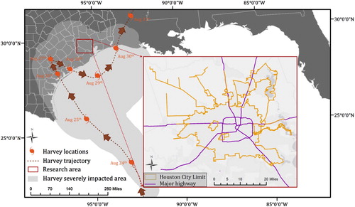
This study selected the Houston Flood on 25th August –to 1st September 2017 as our study case (Figure 1). Affected by Hurricane Harvey, the City of Houston, TX, received at least 800 mm of precipitation within a few days (Blake and Zelinsky, n.d.). The record-breaking rainfall and crippled storm water infrastructures led to a devastating and widespread flood in this city, impacting all aspects of its society. The flood caused an estimate damage of $125 billion and was responsible for at least 64 deaths with over half (36) in the metropolitan area. The study area we chose fully covers the City of Houston.

Figure 1. Hurricane Harvey and the study area of Houston, TX.

2.2. Datasets

2.2.1. Training set of flood and non-flood pictures

The performance of CNNs largely depends on its training set. In this study we developed the comprehensive training sets of flood and non-flood pictures from a variety of sources. The training set of flood pictures comes from two major online sources: searching engine and social media. Via the Google searching engine, 1000 flood pictures are downloaded using the keyword ‘flood’ and manually verified. Via the Baidu searching engine, another set of 1000 flood pictures is extracted using ‘Flooding’ and ‘Hongshui’ (Chinese Pinyin of ‘flooding’). For pictures in social media, we target on three popular, open source social media: Twitter & Instagram and Flickr. A predefined keyword, ‘flood*’, is used for Twitter & Instagram. A total of 29,578 tweets with pictures from 1st December 2015 to 1st December 2017 are downloaded, among which 4400 flood pictures are verified. For Flickr, a tag ‘flooding’ is used and 1000 verified flood pictures are extracted. Tweets in the period from 15th August to 15th September 2017 are not used to exclude pictures about the Houston Flood from the training data selection. In total, 7400 verified flood pictures are collected and served as training inputs of the designed CNN for picture labeling. Note that retweeted pictures derived from social media are not included in this training set. Two-thirds of this dataset are used to train the CNN and one-third is used as the test set for validation analysis.

The non-flood training set contains pictures downloaded from Twitter & Instagram. To make the training sample size balanced, we randomly generate a same size set (7400) of non-flood pictures.

2.2.2. Tweets pool for word sensitivity test

To gain comprehensive understanding of the flood-sensitive words, a total of 1,048,576 tweets from 15th August to 15th September 2017 are collected across the state of Texas using Twitter Stream API (http://dev.twitter.com/streaming) and are stored in a Hadoop computer cluster. A state-wide geolocational restriction provides more stable and reliable volunteered responses, which significantly reduces the impact of the intrinsic noises in Twitter.

2.2.3. Tweets pool for Houston Flood analysis

The geotagged tweets during the Houston Flood in the study area are extracted (retweeted posts are excluded). These tweets have the exact latitude/longitude coordinates (e.g. ‘29.76020, −95.39446’) and therefore, provide high geocoding accuracy for better situational awareness at local level. A total of 38,992 picture-included tweets are extracted from a total of 133,762 streamed tweets during the Houston Flood period (25th August to 1st September). Both of their visual and textual information is analyzed for flood picture selection.

3. Methodology

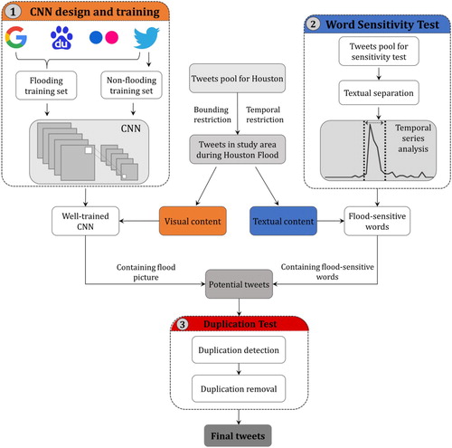
In this study, the proposed methodology consists of three steps: (i) design a CNN and train it based on the flood and non-flood datasets derived from a variety of sources (CNN design and training). The trained CNN is then used to label the flood pictures during the Houston Flood; (ii) automatically extract the flood-sensitive keywords by applying a temporal analysis and use them to trim the CNN classified results (Word Sensitivity Test); (iii) identify the duplicated pictures and only keep the originally posted ones (Duplication Test). The final dataset is a refined collection of flood pictures with locational information during the Houston Flood. Detailed methodology overview is presented in Figure 2.

Figure 2. The workflow of the proposed approach. The methodology is composed of three steps: CNN design and training, word sensitivity test and duplication test.

3.1. CNN design and training

3.1.1. CNN design

A CNN is a hierarchical neural network composed of input and output layers, as well as one or multiple hidden layers. Its form and utility vary upon how those hidden layers are set and realized. In the CNN architecture utilized in this study, the hidden layers consist of the following major types:

• Convolutional layers (CONV): learning features by applying a convolution operation to the input. Each convolutional neuron only accepts features in its receptive field. A convolutional layer is parameterized by four hyperparameters: number of filters ($N_{\mathrm{f}}$), the spatial extent of those filters ($F_{\mathrm{c}\mathrm{o}\mathrm{n}\mathrm{v}}$), convoluting stride ($S_{\mathrm{c}\mathrm{o}\mathrm{n}\mathrm{v}}$) and number of zero padding (P).

• Rectified Linear Unit layers (RELU): introducing nonlinear property via a non-saturating activation function $f\left(x\right)=\mathrm{m}\mathrm{a}\mathrm{x}\left(0,x\right)$, where $x$ represents the input to a neuron.

• Pooling layers (POOL): extracting the most robust and abstract feature within a convolution window in the prior layer and reducing the spatial size of the representation, thus limiting the amount of parameters used in computation and significantly controlling overfitting. It is parameterized by spatial extent ($F_{\mathrm{p}\mathrm{o}\mathrm{o}\mathrm{l}}$) and pooling stride ($S_{\mathrm{p}\mathrm{o}\mathrm{o}\mathrm{l}}$).

• Fully connected layers (FC): flattening high dimensional features by connecting every neuron in the prior layer to next layer. A fully connected layer is parameterized by the number of its neurons ($N_{\mathrm{f}\mathrm{c}}$).

The CNN architecture designed in this study consists of eight layers (six CONVs and two FCs) (Figure 3). First, it resamples an input picture to a 3-D matrix at a 128*128*3 dimension (3 denotes that each picture has three channels, i.e. RGB), then passes it to numerous hidden layers and finally labels it as flood or non-flood. The pattern of hidden layers follows a general ‘CONV–RELU–CONV–RELU–POOL–FC’ scheme. The RELU layers are not presented in Figure 3 for simplicity and legibility of the figure. The double stacking of CONV aims to develop more complicated features before the pooling operation, which inevitably leads to information loss due to layer downsizing. Additionally, the progressive increase of CONV dimensions (64, 128, or 256) allows more possible representative features to be learned, greatly aiding in the richness of feature combinations. Such architectures have been commonly used in studies of machine learning for image processing (Simonyan and Zisserman 2014; Ronneberger et al. 2015).

Figure 3. CNN architecture: the number before ‘@’ denotes the depth of a layer.

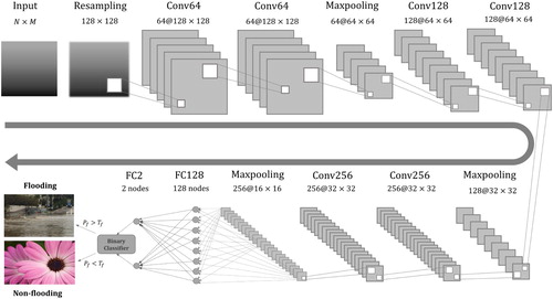
The spatial pooling method in the proposed architecture is Maxpooling (Figure 3), a commonly used pooling method that finds the maximum value from each cluster of neurons at the prior layer (Nagi et al. 2011; Masci et al. 2013). It down-samples the prior layer, hence reducing the number of parameters by selecting a representative value in its matrix, in this case, the largest value. Due to the special characteristics of flood pictures, an additional Dropout layer (D-layer) is added after each CONV layer and the first FC layer (not showing in Figure 3) to prevent the overfitting problem.

The final outputs are two fully connected neurons that contain the probabilities of whether a picture is in the flood category (positive labeling) or non-flood category (negative labeling). $P_f$ denotes the probability of positive labeling and $T_f$ denotes the threshold for positive labeling. The picture is labeled as positive (flood) when $P_f>T_f$, and negative (non-flood) when $P_f<T_f.$

3.1.2. CNN training

To train a CNN, an organized training set is needed to feed the network. In this study, we applied a data augmentation approach to artificially enlarge the dataset, thus reducing the potential overfitting of the network. The data augmentation approach includes horizontal flipping, rotation and zooming. The augmented pictures are shuffled and resampled to a uniform size (128*128*3) before they are passed to the hidden layers. The network then learns different levels of the convoluted layers by constantly adjusting weights of its neurons via a backpropagation algorithm (Riedmiller and Braun 1993). A high-level neural networks API, Keras (Chollet 2015), is used as our coding platform and the parameter settings in our CNN are summarized in Table 1.

Table 1. Parameter settings.

Notation	Parameter description	Value
Feeding phrase
${ϵ}_z$	Zooming factor	$<0.2$
${\theta }_r$	Rotation factor	$<{40}^{\circ }$
$\tau$	Batch size	32
$M$	Input (resampled) image size $\left(M\ast M\right)$	128
N	Number of channels	3
Training phrase
$F_{\mathrm{c}\mathrm{o}\mathrm{n}\mathrm{v}}$	Spatial extent of convolutional filters $(F_{\mathrm{c}\mathrm{o}\mathrm{n}\mathrm{v}}\ast F_{\mathrm{c}\mathrm{o}\mathrm{n}\mathrm{v}})$	3
$S_{\mathrm{c}\mathrm{o}\mathrm{n}\mathrm{v}}$	Convoluting stride$(S_{\mathrm{c}\mathrm{o}\mathrm{n}\mathrm{v}}\ast S_{\mathrm{c}\mathrm{o}\mathrm{n}\mathrm{v}})$	2
$F_{\mathrm{p}\mathrm{o}\mathrm{o}\mathrm{l}}$	Spatial extent of pooling filters ($F_{\mathrm{p}\mathrm{o}\mathrm{o}\mathrm{l}}\ast F_{\mathrm{p}\mathrm{o}\mathrm{o}\mathrm{l}}$)	2
$S_{\mathrm{p}\mathrm{o}\mathrm{o}\mathrm{l}}$	Pooling stride $(S_{\mathrm{p}\mathrm{o}\mathrm{o}\mathrm{l}}\ast S_{\mathrm{p}\mathrm{o}\mathrm{o}\mathrm{l}})$	2
$D_r$	Dropout rate of a D-layer	0.15
P	Zero padding	True^a
$\mathrm{e}$	Maximum epochs	200
$l_r^i$	Initial learning rate	0.00002
$l_r^e$	Progressive learning rate per epoch	$l_r^i/\mathrm{e}\mathrm{p}\mathrm{o}\mathrm{c}\mathrm{h}$^b
$N_{\mathrm{f}\mathrm{c}}^1$	Number of neurons in first FC	128
$N_{\mathrm{f}\mathrm{c}}^2$	Number of neurons in second FC	2

^aTrue zero padding denotes the application of zero padding in CNN training phrase.

^b $l_r^e$ is a progressive variable that updates itself on each epoch.

The total parameters in our designed CNN architecture are 9,538,506. The training of those parameters is accelerated by a NVIDIA GTX 1050 GPU with 8-GB RAM and the Computer Unified Device Architecture (CUDA). The whole training phrase finishes in 10 min.

The well-trained CNN is then applied to label tweet pictures from Houston Flood tweets pool. Tweet pictures in this pool are downloaded using Beautiful Soup, a data scratch library in Python, and they are fed directly to the network to generate their binary labels. Two categories of pictures are labeled: the flood pictures and the non-flood pictures tweeted during the Houston Flood.

3.2. Word sensitivity test

After the flood pictures are labeled by the CNN, we seek to improve the outputs by applying a restriction on their textual information. This process utilizes the textual messages of tweets, aiming to extract all the words with abnormal behaviors from a massive and noisy tweets pool during the Houston Flood. First, a textual separation is applied using white space and hashtag (#) as separators. Those segments after textual separation are organized in a database. However, using white space as separator inevitably allows other symbols (such as exclamation marks) in each segment. Here we remove all these tailing symbols while keeping the meaningful words. For example, ‘flooding!!’ is trimmed as ‘flooding’. Moreover, we only use the segments occurring more than 100 times in the sensitivity analysis. The contribution of less frequently tweeted words is assumed trivial to flood awareness and thus not considered.

Words remained in each segment have different sensitivities regarding the Houston Flood event. Words with a remarkable increase in count exhibit a positive sensitivity to the Flood, while words mentioned remarkably less during the event exhibit a negative sensitivity. In this study, we summarize the word count in a daily level.

Due to the short acquisition period of the test dataset (15th August to 15th September) and the ubiquitous existence of extreme values, we apply a modified Z score to statistically evaluate the sensitiveness for each word. The modified Z score measures the outlier strength or how much a score differs from its median instead of mean, hence less influenced by extreme values. It is computed using the Median Absolute Deviation (MAD), modified from Iglewicz and Hoaglin (1993):(1) $M_i=\frac{C_1\left(x_i-\tilde{x}\right)}{\mathrm{M}\mathrm{A}\mathrm{D}},$(1) where $C_1$ is a constant of 0.6745, $x_i$ denotes the occurrence of a certain word on day $i$. $\tilde{x}$ denotes the sample median and $M_i$ is the modified Z score on day $i$. MAD is calculated by taking the median of the absolute deviations from the median:(2) $\mathrm{M}\mathrm{A}\mathrm{D}=\mathrm{m}\mathrm{e}\mathrm{d}\mathrm{i}\mathrm{a}\mathrm{n}\left\{\left|x_i-\tilde{x}\right|\right\}.$(2)

Specifically, when MAD = 0, the function is modified as(3) $M_i=\frac{C_2\left(x_i-\tilde{x}\right)}{\mathrm{M}\mathrm{e}\mathrm{a}\mathrm{n}\mathrm{A}\mathrm{D}},$(3) (4) $\mathrm{M}\mathrm{e}\mathrm{a}\mathrm{n}\mathrm{A}\mathrm{D}=\mathrm{m}\mathrm{e}\mathrm{a}\mathrm{n}\left\{\left|x_i-\tilde{x}\right|\right\},$(4) where $C_2$ is a constant of 0.7966. Similar as Equation (2), MeanAD is calculated by taking the mean of the absolute deviations from the median.

The modified Z scores provide the intensity of how daily count of a word deviates from the median in its time series from 15th August to 15th September. Given a single word, its overall flood sensitiveness to the Houston Flood, $S_f$, is the absolute value of its accumulated modified Z scores during the Flood period (25th August to 1st September):(5) $S_f=\left|\sum _i{M}_i\right|\left(i\in \left[25\mathrm{t}\mathrm{h}\mathrm{A}\mathrm{u}\mathrm{g}\mathrm{u}\mathrm{s}\mathrm{t},1st\mathrm{S}\mathrm{e}\mathrm{p}\mathrm{t}\mathrm{e}\mathrm{m}\mathrm{b}\mathrm{e}\mathrm{r}\right]\right)$(5) To bifurcate sensitive and non-sensitive words, we rank all the words based on accumulated modified Z score. Specifically, words with top 200 $S_f$ are selected as flood-sensitive words.

For the CNN-extracted flood pictures during the Houston Flood, their textual information accompanying each tweet goes through the sensitivity test described above.

It is assumed that tweets of wrongly classified flood pictures are unlikely to contain flood-sensitive words. Therefore, only tweets that contain both labeled flood pictures and flood-sensitive words are selected into the refined tweets pool.

3.3. Duplication test

After the application of visual and textual restriction, tweets that contain positively labeled pictures and sensitive words were extracted. However, it is commonly observed that duplicate pictures are equally selected. For example, a flood picture may be shared multiple times by different users during the flood event. Unlike the original post (the first in timeline), the locational information of the tweets posting the duplicate pictures does not reflect the location and time when the picture is taken and therefore, does not help situational awareness. This process aims to identify and remove the duplicate pictures from the extracted flood pictures.

Given a picture pair, the duplicate identification algorithm computes the summation of the absolute difference in each channel:(6) $S_{\mathrm{s}\mathrm{c}\mathrm{o}\mathrm{r}\mathrm{e}}=\sum _n^N\sum _{i,j}|O_{i,j}^n-K_{i,j}^n|$(6) where $\mathrm{O}$ and $\mathrm{K}$ represent the two pictures being compared. $i$ and $j$ are the row and column respectively. $n$ denotes the channel number and $N$ ($N=3$) denotes the RGB channels of each picture. To make this process less computational expensive, all pictures are resampled to a size of 128*128*3 before feeding to the duplication test.

The $S_{\mathrm{s}\mathrm{c}\mathrm{o}\mathrm{r}\mathrm{e}}$ represents the similarity of the picture pair. A $S_{\mathrm{s}\mathrm{c}\mathrm{o}\mathrm{r}\mathrm{e}}$ with 0 means a perfect duplication. The higher the $S_{\mathrm{s}\mathrm{c}\mathrm{o}\mathrm{r}\mathrm{e}}$ is, the less similarity the picture pair has. In this study, only perfect duplications are considered. When a picture pair is identified as duplicate, the tweet with a later posting time is removed.

With a repetitive process, all tweets with duplicate pictures are removed. The final output of this study is a collection of flood-related tweets supported by their posted flood pictures.

3.4. Performance evaluation

A set of metrics, including the accuracy, loss, precision, recall and $F_1$ score, are used to evaluate the tweet labeling performance of using visual information only (CNN) and using both visual and textual information (CNN coupling with flood-sensitive words). For each evaluation, the classified results fall into four categories:

• True positive (TP): the number of tweets correctly identified as flood tweets

• False positive (FP): the number of tweets incorrectly identified as flood tweets

• True negative (TN): the number of tweets correctly identified as non-flood tweets

• False negative (FN): the number of tweets incorrectly identified as non-flood tweets.

The accuracy is frequently used to measure the ability of a model to differentiate binary classes, i.e. flood and non-flood in this study. It is calculated by combining TP, FP, TN, and FN:(7) $\mathrm{A}\mathrm{c}\mathrm{c}\mathrm{u}\mathrm{r}\mathrm{a}\mathrm{c}\mathrm{y}=\frac{\mathrm{T}\mathrm{P}+\mathrm{T}\mathrm{N}}{\mathrm{T}\mathrm{P}+\mathrm{T}\mathrm{N}+\mathrm{F}\mathrm{P}+\mathrm{F}\mathrm{N}}$(7) The loss function is binary cross-entropy loss. It measures the performance of a binary labeling model as(8) $\mathrm{L}\mathrm{o}\mathrm{s}\mathrm{s}=-\left(y\mathrm{l}\mathrm{o}\mathrm{g}\left(p\right)+\left(1-y\right)\log \left(1-p\right)\right),$(8) where $y$ is a binary indicator (0 or 1). It equals 1 when a picture is labeled as flood and 0 when labeled as non-flood. $p$ represents the predicted probability of a picture being labeled as flood.

Precision and recall are two indices commonly used in machine learning to quantify the performance of an algorithm. Precision measures the proportion of correctly identified flood pictures among all positive labels, or a measure of overestimation. Recall measures the proportion of correctly identified flood pictures among all flood pictures, i.e. a measure of omission:(9) $\mathrm{P}\mathrm{r}\mathrm{e}\mathrm{c}\mathrm{i}\mathrm{s}\mathrm{i}\mathrm{o}\mathrm{n}=\frac{\mathrm{T}\mathrm{P}}{\mathrm{T}\mathrm{P}+\mathrm{F}\mathrm{P}},$(9) (10) $\mathrm{R}\mathrm{e}\mathrm{c}\mathrm{a}\mathrm{l}\mathrm{l}=\frac{\mathrm{T}\mathrm{P}}{\mathrm{T}\mathrm{P}+\mathrm{F}\mathrm{N}}.$(10)

Leveraging the precision and recall, the $F_1$ score is an index that measures the overall accuracy of a binary classifier. It is calculated as(11) $F_1=\frac{2}{{\displaystyle \frac{1}{\mathrm{p}\mathrm{r}\mathrm{e}\mathrm{c}\mathrm{i}\mathrm{s}\mathrm{i}\mathrm{o}\mathrm{n}}+\frac{1}{\mathrm{r}\mathrm{e}\mathrm{c}\mathrm{a}\mathrm{l}\mathrm{l}}}}$(11) The $F_1$ score reaches its best value at 1 (perfect precision and recall) and the worst at 0.

4. Results and discussion

4.1. CNN performance

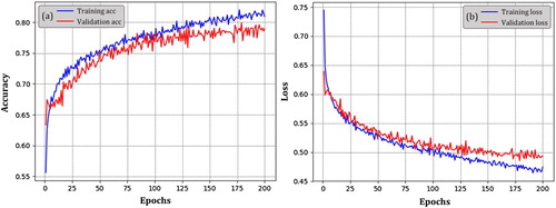
Accelerated by GPU and CUDA architecture, the designed CNN finished the training phrase in 10 min and 43 s through 200 epochs. The CNN reached an accuracy around 80% in both training and test sets (Figure 4a). Consecutive and stable training loss was observed throughout the training phrase (Figure 4b). The implementation of D-layer following each CONV layer has been proven efficient as it successfully prevents the model from being overfitted. Given the special characteristics in flood pictures and the ubiquitous existence of pictures with a similar texture (Feng and Sester 2018), the accuracy around 80% using CNN alone is considered acceptable compared with other flood picture classification results (Avgerinakis et al. 2017; Bischke et al. 2017).

Figure 4. Training accuracy and loss of designed CNN architecture on flooding and non-flooding dataset supported by GTX 1050 GPU and CUDA.

After the training, the CNN model with the optimal weight settings in its neurons was stored and then used to classify 38,992 tweet pictures derived from a total of 133,762 tweets during the Houston Flood (25th August to 1st September). To understand the performance of our model in this largely unbalanced Houston tweet dataset (the ratio between the number of flooding and non-flood pictures is much less than a balanced ratio 0.5), we gradually increased threshold $T_f$ from 0.50 to 0.95 and recorded its performance with a varying $T_f$in positive labels (Figure 5). As expected, with the increasing of $T_f$, number of pictures with positive labels decrease dramatically (Figure 5a). Number of True positives (TPs) and False Positives (FPs) also decreases following the increasing $T_f$. For instance, when $T_f=0.5$, 2545 pictures were labeled positive with 1301 TPs and 1244 FPs, while when $T_f=0.7$, only 755 pictures were labeled positive with 663 TPs and 92 FPs. A larger $T_f$ indicates a stricter criterion for positive labeling and results in a higher positive labeling precision at the expense of lower recall of positive labels (Figure 5b).

Figure 5. CNN performance with different ${\mathit{T}}_{\mathit{f}}$: (a) number of pictures classified as positive (flooding), verified as positive (TP) and verified as negative (FP) given different $T_f$ and (b) trend of precision and recall given different $T_f$.

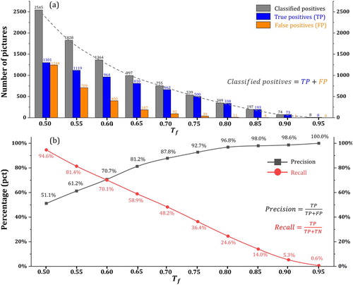
Figure 5(b) reveals strong negative correlation between precision and recall in positive labels, which demonstrates the dilemma of $T_f$ setting if we purely rely on CNN for recognizing flood pictures. A lower $T_f$, for instance 0.5, leads to a high recall but low precision while a higher $T_f$, for instance 0.70, results in a low recall but high precision. In both cases, additional efforts are needed either to manually exclude the misclassified positive labels or include the misclassified negative labels. More details of negative labeling can be seen in the summary (Table 2).

Table 2. CNN labeling result.

	Classified as positive			Classified as negative			Evaluation (positive)
$T_f$	Total	TPs	FPs (Type I)	Total	TNs	FNs (Type II)	Precision (%)	Recall (%)
0.5	2545	1301	1244	36,447	36,373	74	51.1	94.6
0.55	1828	1119	709	37,164	36,908	256	61.2	81.4
0.6	1364	964	400	37,628	37,217	411	70.7	70.1
0.65	997	810	187	37,995	37,430	565	81.2	58.9
0.7	755	663	92	38,237	37,525	712	87.8	48.2
0.75	539	500	39	38,453	37,578	875	92.8	36.3
0.8	349	338	11	38,643	37,606	1037	96.8	24.6
0.85	197	193	4	38,795	37,613	1182	98.0	14.0
0.9	74	73	1	38,918	37,616	1302	98.6	05.3
0.95	8	8	0	38,984	37,617	1367	100.0	00.6

In a flood event, a higher recall (less FNs) is preferred as it leads to a better coverage of true flood pictures, which is of great importance for agencies to gain a comprehensive situational awareness and for responders to evacuate as many people as possible. Given the importance of recall rate in flood events, a lower $T_f$ value is preferred in this case. The low precision problem introduced by a low $T_f$ value is compensated in next step.

4.2. Flood-sensitive words extraction

After the segmentation and tailing symbol removal of the tweeted messages across Texas during the Flood, 6415 words occurring over 100 times are remained in the selection. These segments contain not only regular English words but also commonly used modal particles such as ‘OMG’. The summation of the modified Z score for each word $S_f$, represents the sensitivity of that word to the flood event. We manually categorize those words into four different sensitive levels based on their $S_f$ value. Top 200 words with highest $S_f$ value (ranging from 15 to 200) are then selected as flood-sensitive words.

In Figure 6, the first tier of sensitive levels ($100<S_f<200$) includes words such as ‘boat’ ($S_f=138.95$), ‘safe’ ($S_f=126.57$) and ‘raining’ ($S_f=199.77$). Words in this category were mentioned extremely more frequently during the Houston Flood. ‘flood*’, the most commonly used keyword to extract flood tweet in past studies (Li et al. 2018; Huang et al. 2018b), is in the second tier ($50<S_f<100$) (the $S_f$ for ‘flood*’ is the average $S_f$ for all the variations of ‘flood’). Other words in this category include ‘stuck’, ‘stay’, ‘shelters’, ‘storm’, etc. It should be noted that tweets bearing sensitive words like ‘stuck’ or ‘stay’ may provide timely geolocational information about where potential flood victims are trapped. This information can greatly aid authorities and local responders for rapid evacuation. Tweets containing words in the third ($25<S_f<50$) and fourth ($15<S_f<25$) tiers are also strongly flood related. However, they are largely ignored in traditional flood-related tweets selection processes, which only utilizes limited predefined keywords.

Figure 6. Temporal distribution of selected flood-sensitive words (${\mathit{S}}_{\mathit{f}}>15$). The X-axis and Y-axis in each subfigure denote time (from 15th August to 15th September in 2017) and number of tweets (count) respectively. Number of tweets for each word has been scaled for better visualization and comparison.

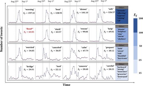
By quantifying the sensitivity of each word and creating an automatic, large pool of sensitive words for a flood event, this study greatly expands the scope of traditional flood selection process. As revealed in Figure 6, much more keywords are identified, which dramatically reduces the underestimation of flood tweets in previous studies. These extracted flood-sensitive words are used to refine the CNN-labeled flood pictures.

4.3. Refining CNN results based on sensitive words

After applying restrictions of sensitive words in textual tweets to address the low precision problem in CNN-labeled flood pictures, we observed a significant reduction in total positive labels after refining the CNN results with sensitive words (Table 3). After applying the textual restriction, the number of FPs dropped while the number of TPs remained relatively the same. The reduction is more dramatic at lower $T_f$ thresholds. For instance, when $T_f=0.5$, the number of FPs experienced a huge decrease from 1244 in the CNN labeling model itself to 183 after refining with sensitive words. Oppositely, the reduction of TPs is minimal (from 1301 to 1272). However, at a larger $T_f$ value, the significant decrease in FPs over TPs becomes less obvious or even reversed. An extremely large $T_f$ value, is not meaningful due to the limited number of TPs it can extract. The significant decrease in FPs over TPs when $T_f$ is low indicates that coupling visual information with textual information can considerably remove non-flood tweets while keeping a majority of true flood tweets.

Table 3. Positive label (TPs and FPs) statistics in CNN only and CNN refined by sensitive words.

	CNN only			CNN refined by sensitive words
$T_f$	Total extraction	TPs	FPs	Total extraction	TPs	FPs
0 . 5	2545	1301	1244	1455	1272	183
0.55	1828	1119	709	1273	1141	132
0.6	1364	964	400	972	883	89
0.65	997	810	187	812	739	73
0.7	755	663	92	658	608	50
0.75	539	500	39	513	472	41
0.8	349	338	11	321	294	27
0.85	197	193	4	185	170	15
0.9	74	73	1	67	65	2
0.95	8	8	0	8	7	1

As shown in Table 4, the precision of the refined CNN model with sensitive words improves remarkably compared with the precision in using CNN only, especially when $T_f=0.5$ where the precision increased by 36.3% (from 51.1% to 87.4%). The same pattern can be observed in all low $T_f$. Along with the significant boost in precision, the recall rate remains in a high level. An average that considers both precision and recall, $F_1$, also observes noticeable increased performance especially when $T_f$ is low, which indicates more robustness in the model after refining the CNN results with sensitive words. To ensure the highest recall rate, we set parameter $T_f$ as 0.5 for flood picture labeling in the Houston Flood.

Table 4. Precision, recall and $F_1$ score in CNN only and CNN refined by sensitive words.

	CNN only			CNN refined by sensitive words
$T_f$	Precision	Recall	$F_1$	Precision	Recall	$F_1$
0 . 5	51.1%	94.6%	0.664	87.4%	92.5%	0.899
0.55	61.2%	81.4%	0.699	89.6%	83.0%	0.862
0.6	70.7%	70.1%	0.704	90.8%	64.2%	0.752
0.65	81.2%	58.9%	0.683	91.0%	53.7%	0.676
0.7	87.8%	48.2%	0.622	92.4%	44.2%	0.598
0.75	92.8%	36.4%	0.522	92.0%	34.3%	0.500
0.8	96.8%	24.6%	0.392	91.6%	21.4%	0.347
0.85	98.0%	14.0%	0.246	91.9%	12.4%	0.218
0.9	98.6%	5.3%	0.101	97.0%	4.7%	0.902
0.95	100.0%	0.6%	0.012	87.5%	0.5%	0.101

In short, after applying the textual restriction on CNN classified results, we significantly increase the precision while keep the recall in a high level in low $T_f$. We successfully keep most TPs in the selection and remove majority of FPs which were wrongly classified by CNN.

4.4. Duplication removal and the flood tweets geotagging

After applying the visual-textual restriction, the figure-attached tweets that satisfy both requirements were selected and stored in a potential tweets pool. With the algorithm described in Section 3.3, we identified a total of 214 duplicate pictures in the potential tweets pool of the Houston Flood. Figure 7 shows several examples of the detected originals and their duplications in the timeline (the posting sequence). The originals, posted first in the timeline, are represented in red dots, while the duplications in blue dot. We found that pictures with the most duplications were those people used to share their concerns, for example the picture of ‘PRAY FOR HOUSTON’ in Figure 7, which has been repeatedly posted 34 times during the flood period. Exaggerated flood pictures that do not belong to the study area or modified flood pictures for amusement were also found heavily duplicated.

Figure 7. Examples of selected originals and their duplications presented in their timeline. Only the originals (the first in timeline) were kept in the final selection.

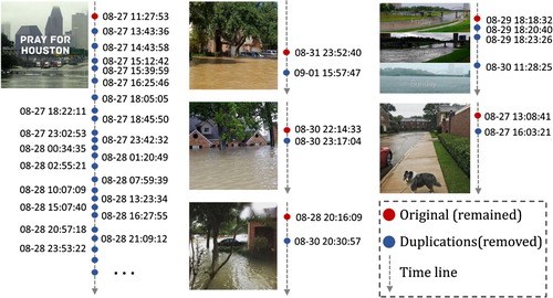
As expected, flood pictures in the original post often well indicated the flooded situation in the posted locations. The duplicate pictures fail to provide timely and accurate locational information for flood awareness. By only keeping the original post, this study significantly reduced the number of these duplicate pictures. The resulted tweets pool guarantees a high spatio-temporal relevance, which renders more confidence when assessing flood extent, evaluating flood damage and gauging evacuation.

The final pool contains the duplication-removed tweets (a total of 1241) in the Houston Flood that meet both visual and textual restrictions. A point map of these tweets is displayed in Figure 8. Each tweet indicates the high possibility of being flooded at its location. In general, the distribution of final selection correlates well with population density as densely populated area tends to have more Twitter users, and therefore, generates more tweets.

Figure 8. Selected examples of final tweets geotagging.

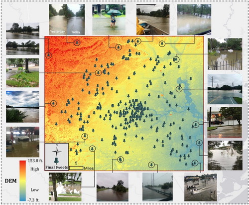
Some geotagged tweets contain useful water height information that can be drawn from either visual content, textual content or both. If validated, these water heights could serve as hundreds of additional ‘rivers gauges’ that are widely distributed across the study area, providing valuable flooding awareness in such a huge area in a timely manner. The water height information derived from a huge volume of automatically generated flood tweets could largely compensate the limitations of river gauges due to its spatial isolated characteristic and water overflow induced data missing problem. Besides, given their real-time merit, the extracted flood tweets provide timely locational flood awareness, significantly assisting rapid response by local authorities and first responders to provide evacuations to those who need. Moreover, supported with local Digital Elevation Model (DEM), the geolocational information rendered by extracted flood tweets can serve as an important input to generate timely flood extent map with a large spatial coverage, significantly aiding the understanding of flood situation in a holistic way.

5. Conclusion

Nowadays social media such as Twitter has become a popular data source for rapid flood evaluation. Serving as an in situ source, the highly up-to-date responses and large coverage from those citizen sensors greatly benefit a variety of real-time flood analysis. Relying on both visual and textual information a tweet provides, this study presents an automated approach to tagging flood tweets during a flood event. It could be easily generalized to other flood cases with a larger Twitter sample. We collected a comprehensive training dataset of flood pictures from various online searching engines and social media and used it to train our designed CNN model. The CNN labeling results in the Houston Flood were later refined by flood-sensitive words derived from a word sensitivity test. The remaining tweets that satisfied both visual and textual requirements were further trimmed by a duplication test model. Only the originally posted tweets were remained, which composed the final tweets pool of the metropolitan Houston during the flood.

The primary findings of this study include: (i) While the commonly used keywords can effectively extract flood tweets, automatic selection of sensitive words is found practical to ensure a better flood tweets pool; (ii) The temporal distribution patterns vary in different words and the summation of the modified Z score during the flood period can effectively quantify the sensitivity of a certain word; (iii) The tradeoff between precision and recall in a CNN picture classifier can be compensated by coupling CNN classified results with flood-sensitive words, leading to a significant precision improvement while keeping the recall in a high level; and (iv) The removal of duplicated pictures guarantees the inclusion of more spatio-temporal flood relevant tweets.

The automation of geotagging flood tweets can greatly improve traditional selection process which is labor- and time-consuming. The usage of statistically extracted flood-sensitive words instead of a few predefined keywords significantly expands the searching scope and ensures a better coverage of selected flood tweets from millions of tweets in the pool. The proposed method could be generalized to other events and seed a wide range of social media based disaster studies.

Disclosure statement

No potential conflict of interest was reported by the authors.

ORCID

Xiao Huang http://orcid.org/0000-0002-4323-382X

Cuizhen Wang http://orcid.org/0000-0002-0306-9535

References

- Avgerinakis, K., A. Moumtzidou, S. Andreadis, E. Michail, I. Gialampoukidis, S. Vrochidis, and I. Kompatsiaris. 2017. “Visual and Textual Analysis of Social Media and Satellite Images for Flood Detection@ Multimedia Satellite Task MediaEval 2017.” Proceedings of the working notes proceeding MediaEval workshop, Dublin, Ireland (pp. 13–15).
- Bischke, B., P. Bhardwaj, A. Gautam, P. Helber, D. Borth, and A. Dengel. 2017. “Detection of Flooding Events in Social Multimedia and Satellite Imagery Using Deep Neural Networks.” Proceedings of the working notes proceeding MediaEval workshop, Dublin, Ireland (pp. 13–15).
- Blake, E., and D. Zelinsky. n.d. “National Hurricane Center Tropical Cyclone Report: Hurricane Harvey (Rep.).” Accessed May 11, 2018 from National Hurricane Center Website: https://www.nhc.noaa.gov/data/tcr/AL092017_Harvey.pdf.
- Boiman, O., E. Shechtman, and M. Irani. 2008. “Defense of Nearest-Neighbor Based Image Classification.” IEEE conference on Computer Vision and Pattern Recognition (CVPR'08) (pp. 1–8). IEEE.
- Caragea, C., A. C. Squicciarini, S. Stehle, K. Neppalli, and A. H. Tapia. 2014. “Mapping Moods: Geo-Mapped Sentiment Analysis During Hurricane Sandy.” ISCRAM.
- Chew, C., and G. Eysenbach. 2010. “Pandemics in the age of Twitter: Content Analysis of Tweets During the 2009 H1N1 Outbreak.” PloS One 5 (11): e14118. doi: 10.1371/journal.pone.0014118
- Chollet, F. (2015) . Keras. https://keras.io/.
- Ciregan, D., U. Meier, and J. Schmidhuber. 2012. “Multi-Column Deep Neural Networks for Image Classification.” IEEE conference on Computer Vision and Pattern Recognition (CVPR'12), June (pp. 3642–3649). IEEE.
- Ciresan, D. C., U. Meier, J. Masci, L. Maria Gambardella, and J. Schmidhuber. 2011. “Flexible, High Performance Convolutional Neural Networks for Image Classification.” IJCAI'11 Proceedings of the 22nd international joint conference on Artificial Intelligence, Barcelona, Catalonia, Spain, July 16–22 (pp. 1237–1242).
- De Albuquerque, J. P., B. Herfort, A. Brenning, and A. Zipf. 2015. “A Geographic Approach for Combining Social Media and Authoritative Data Towards Identifying Useful Information for Disaster Management.” International Journal of Geographical Information Science 29 (4): 667–689. doi: 10.1080/13658816.2014.996567
- Dredze, M. 2012. “How Social Media Will Change Public Health.” IEEE Intelligent Systems 27 (4): 81–84. doi: 10.1109/MIS.2012.76
- Fakhari, A., and A. M. E. Moghadam. 2013. “Combination of Classification and Regression in Decision Tree for Multi-Labeling Image Annotation and Retrieval.” Applied Soft Computing 13 (2): 1292–1302. doi: 10.1016/j.asoc.2012.10.019
- Feick, R., and S. Roche. 2013. “Understanding the Value of VGI.” In Crowdsourcing Geographic Knowledge, 15–29. Dordrecht: Springer.
- Feng, Y., and M. Sester. 2018. “Extraction of Pluvial Flood Relevant Volunteered Geographic Information (VGI) by Deep Learning from User Generated Texts and Photos.” ISPRS International Journal of Geo-Information 7 (2): 39. doi: 10.3390/ijgi7020039
- Fohringer, J., D. Dransch, H. Kreibich, and K. Schröter. 2015. “Social Media as an Information Source for Rapid Flood Inundation Mapping.” Natural Hazards and Earth System Sciences 15 (12): 2725–2738. doi: 10.5194/nhess-15-2725-2015
- Goodchild, M. F. 2007. “Citizens as Sensors: The World of Volunteered Geography.” GeoJournal 69 (4): 211–221. doi: 10.1007/s10708-007-9111-y
- Herfort, B., J. P. de Albuquerque, S. J. Schelhorn, and A. Zipf. 2014. “Exploring the Geographical Relations Between Social Media and Flood Phenomena to Improve Situational Awareness.” Connecting a Digital Europe Through Location and Place (pp. 55–71). Cham: Springer.
- Ho, T. Y., P. M. Lam, and C. S. Leung. 2008. “Parallelization of Cellular Neural Networks on GPU.” Pattern Recognition 41 (8): 2684–2692. doi: 10.1016/j.patcog.2008.01.018
- Huang, X., C. Wang, and Z. Li. 2018a. “A Near Real-Time Flood Mapping Approach by Integrating Social Media and Post-Event Satellite Imagery.” Annals of GIS, 24(2), 113–123. doi: 10.1080/19475683.2018.1450787
- Huang, X., C. Wang, and Z. Li. 2018b. “Reconstructing Flood Inundation Probability by Enhancing Near Real-Time Imagery with Real-Time Gauges and Tweets.” IEEE Transactions on Geoscience and Remote Sensing, 56(8), 4691–4701. doi: 10.1109/TGRS.2018.2835306
- Iglewicz, B., and D. C. Hoaglin. 1993. How to Detect and Handle Outliers. Vol. 16. Milwaukee, WI: ASQC Quality Press.
- Jancsary, J., S. Nowozin, T. Sharp, and C. Rother. 2012. “Regression Tree Fields – An Efficient, Non-Parametric Approach to Image Labeling Problems.” 2012 IEEE conference on Computer Vision and Pattern Recognition (CVPR) (pp. 2376–2383). IEEE.
- Krizhevsky, A., I. Sutskever, and G. E. Hinton. 2012. “ImageNet Classification with Deep Convolutional Neural Networks.” Proceedings of the 25th International Conference on Neural Information Processing Systems, Lake Tahoe, NV, December 3–6 (pp. 1097–1105).
- Lachlan, K. A., P. R. Spence, X. Lin, and M. Del Greco. 2014. “Screaming Into the Wind: Examining the Volume and Content of Tweets Associated with Hurricane Sandy.” Communication Studies 65 (5): 500–518. doi: 10.1080/10510974.2014.956941
- Li, Z., C. Wang, C. T. Emrich, and D. Guo. 2018. “A Novel Approach to Leveraging Social Media for Rapid Flood Mapping: A Case Study of the 2015 South Carolina Floods.” Cartography and Geographic Information Science 45 (2): 97–110. doi: 10.1080/15230406.2016.1271356
- Longueville, B. D., G. Luraschi, P. Smits, S. Peedell, and T. D. Groeve. 2010. “Citizens as Sensors for Natural Hazards: A VGI Integration Workflow.” Geomatica 64 (1): 41–59.
- Martín, Y., Z. Li, and S. L. Cutter. 2017. “Leveraging Twitter to Gauge Evacuation Compliance: Spatiotemporal Analysis of Hurricane Matthew.” PLoS One 12 (7): e0181701. doi: 10.1371/journal.pone.0181701
- Masci, J., A. Giusti, D. Ciresan, G. Fricout, and J. Schmidhuber. 2013. “A Fast Learning Algorithm for Image Segmentation with Max-Pooling Convolutional Networks.” 20th IEEE International Conference on Image Processing (ICIP'13) (pp. 2713–2717). IEEE.
- McCann, S., and D. G. Lowe. 2012. “Local Naive Bayes Nearest Neighbor for Image Classification.” 2012 IEEE conference on Computer Vision and Pattern Recognition (CVPR), June (pp. 3650–3656). IEEE.
- McDougall, K. 2011. “Using Volunteered Information to Map the Queensland Floods.” Proceedings of the 2011 Surveying and Spatial Sciences Conference: Innovation in Action: Working Smarter (SSSC'11) (pp. 13–23). Surveying and Spatial Sciences Institute.
- Nagi, J., F. Ducatelle, G. A. Di Caro, D. Cireşan, U. Meier, A. Giusti, and L. M. Gambardella. 2011. “Max-Pooling Convolutional Neural Networks for Vision-Based Hand Gesture Recognition.” 2011 IEEE International Conference on Signal and Image Processing Applications (ICSIPA), November (pp. 342–347). IEEE.
- Ovtcharov, K., O. Ruwase, J. Y. Kim, J. Fowers, K. Strauss, and E. S. Chung. 2015. “Accelerating Deep Convolutional Neural Networks Using Specialized Hardware.” Microsoft Research Whitepaper 2 (11): 1–4.
- Pinheiro, P., and R. Collobert. 2014. “Recurrent Convolutional Neural Networks for Scene Labeling.” International Conference on Machine Learning 32: 82–90.
- Riedmiller, M., and H. Braun. 1993. “A Direct Adaptive Method for Faster Backpropagation Learning: The RPROP Algorithm.” IEEE international conference on Neural Networks (pp. 586–591). IEEE.
- Ronneberger, O., P. Fischer, and T. Brox. 2015. “U-NET: Convolutional Networks for Biomedical Image Segmentation.” International conference on Medical Image Computing and Computer-assisted Intervention, October (pp. 234–241). Cham: Springer.
- Sakaki, T., M. Okazaki, and Y. Matsuo. 2010. “Earthquake Shakes Twitter Users: Real-Time Event Detection by Social Sensors.” Proceedings of the 19th International Conference on World Wide Web, April (pp. 851–860). ACM.
- Schnebele, E., G. Cervone, S. Kumar, and N. Waters. 2014. “Real Time Estimation of the Calgary Floods Using Limited Remote Sensing Data.” Water 6 (2): 381–398. doi: 10.3390/w6020381
- Schnebele, E., and N. Waters. 2014. “Road Assessment After Flood Events Using Non-Authoritative Data.” Natural Hazards and Earth System Sciences 14 (4): 1007. doi: 10.5194/nhess-14-1007-2014
- Simard, P. Y., D. Steinkraus, and J. C. Platt. 2003, August. “Best Practices for Convolutional Neural Networks Applied to Visual Document Analysis.” ICDAR 3: 958–962.
- Simonyan, K., and A. Zisserman. 2014. “Very Deep Convolutional Networks for Large-Scale Image Recognition.” arXiv preprint arXiv:1409.1556.
- Skoric, M., N. Poor, P. Achananuparp, E. P. Lim, and J. Jiang. 2012. “Tweets and Votes: A Study of the 2011 Singapore General Election.” 45th Hawaii International Conference on System Science (HICSS'12), January (pp. 2583–2591). IEEE.
- Small, T. A. 2011. “What the Hashtag? A Content Analysis of Canadian Politics on Twitter. Information.” Communication & Society 14 (6): 872–895. doi: 10.1080/1369118X.2011.554572
- Suykens, J. A., and J. Vandewalle. 1999. “Least Squares Support Vector Machine Classifiers.” Neural Processing Letters 9 (3): 293–300. doi: 10.1023/A:1018628609742
- Triglav-Čekada, M., and D. Radovan. 2013. “Using Volunteered Geographical Information to Map the November 2012 Floods in Slovenia.” Natural Hazards and Earth System Sciences 13 (11): 2753. doi: 10.5194/nhess-13-2753-2013
- Vieweg, S., A. L. Hughes, K. Starbird, and L. Palen. 2010. “Microblogging During Two Natural Hazards Events: What Twitter May Contribute to Situational Awareness.” Proceedings of the SIGCHI conference on Human Factors in Computing Systems, April (pp. 1079–1088). ACM.
- Wang, C., Z. Li, and X. Huang. 2018. “Geospatial Assessment of Wetness Dynamics in the October 2015 SC Flood with Remote Sensing and Social Media.” Southeastern Geographer 58 (2): 164–180. doi: 10.1353/sgo.2018.0020
- Wang, J., Y. Yang, J. Mao, Z. Huang, C. Huang, and W. Xu. 2016. “CNN–RNN: A Unified Framework for Multi-Label Image Classification.” 2016 IEEE conference on Computer Vision and Pattern Recognition (CVPR) (pp. 2285–2294). IEEE.
- Wei, Z., J. Chen, W. Gao, B. Li, L. Zhou, Y. He, and K. F. Wong. 2013. “An Empirical Study on Uncertainty Identification in Social Media Context.” Proceedings of the 51st Annual Meeting of the Association for Computational Linguistics (Volume 2: Short Papers) (pp. 58–62).
- Wei, Y., W. Xia, M. Lin, J. Huang, B. Ni, J. Dong, and S. Yan. 2016. “HCP: A Flexible CNN Framework for Multi-Label Image Classification.” IEEE Transactions on Pattern Analysis and Machine Intelligence 38 (9): 1901–1907. doi: 10.1109/TPAMI.2015.2491929
- Wu, K., and K. H. Yap. 2006. “Fuzzy SVM for Content-Based Image Retrieval: A Pseudo-Label Support Vector Machine Framework.” IEEE Computational Intelligence Magazine 1 (2): 10–16. doi: 10.1109/MCI.2006.1626490