The grey-green divide: multi-temporal analysis of greenness across 10,000 urban centres derived from the Global Human Settlement Layer (GHSL)

ABSTRACT

The presence of green spaces within city centres has been recognized as a valuable component of the city landscape. Vegetation provides a variety of benefits including energy saving, improved air quality, reduced noise pollution, decreased ambient temperature and psychological restoration. Evidence also shows that the amount of vegetation, known as ‘greenness’, in densely populated areas, can also be an indicator of the relative wealth of a neighbourhood. The ‘grey-green divide’, the contrast between built-up areas with a dominant grey colour and green spaces, is taken as a proxy indicator of sustainable management of cities and planning of urban growth. Consistent and continuous assessment of greenness in cities is therefore essential for monitoring progress towards the United Nations Sustainable Development Goal 11. The availability of multi-temporal greenness information from Landsat data archives together with data derived from the city centres database of the Global Human Settlement Layer (GHSL) initiative, offers a unique perspective to quantify and analyse changes in greenness across 10,323 urban centres all around the globe. In this research, we assess differences between greenness within and outside the built-up area for all the urban centres described by the city centres database of the GHSL. We also analyse changes in the amount of green space over time considering changes in the built-up areas in the periods 1990, 2000 and 2014. The results show an overall trend of increased greenness between 1990 and 2014 in most cities. The effect of greening is observed also for most of the 32 world megacities. We conclude that using simple yet effective approaches exploiting open and free global data it is possible to provide quantitative information on the greenness of cities and its changes over time. This information is of direct interest for urban planners and decision-makers to mitigate urban related environmental and social impacts.

KEYWORDS:

• Global human settlement layer
• greenness
• Landsat data records
• degree of urbanization
• urban centres
• built-up areas
• sustainable development goal 11

1. Introduction

The presence of green spaces within city centres has been recognized as an essential component of the urban environment (Lee, Jordan, and Horsley 2015). Green spaces in cities are mostly composed of semi-natural vegetation cover e.g. street plantation, lawns, parks, gardens, forests, green roofs (Gan et al. 2014). These spaces typically provide valuable ecosystem services and play an irreplaceable role in the enhancement of the urban environment. Notable among these benefits are the improved air quality (Davies et al. 2008), the interception of surface water runoff (Walsh, Fletcher, and Burns 2012), the reduction of urban heat islands and energy demands (Yuan 2017) and the provision of recreational opportunities for city dwellers (Chen and Jim 2008). Evidence also shows that the amount of vegetation, known as ‘greenness’, in densely populated areas, can also be an indicator of the relative wealth of a neighbourhood (Landry and Chakraborty 2009).

The ‘grey-green divide’, the contrast between built-up areas with a dominant grey colour and green spaces, is proposed as a proxy indicator of sustainable management of cities and planning of urban growth. Improving availability of green spaces in cities is considered in the United Nations Sustainable Development Goals (SDG), specifically in target 11.7, which aims to achieve the following: ‘By 2030, provide universal access to safe, inclusive and accessible, green and public spaces, in particular for women and children, older persons and persons with disabilities’ (United Nations 2015). Characterizing and understanding the changes and trends in greenness and its relationship with the development and dynamics of human settlements can help guide sustainable urban development (Gan et al. 2014).

Over the past two decades, studies have found that changes in green spaces are essentially related to urbanization processes that can take the form of either densification of the urban core or urban sprawl in the fringe of cities and agricultural lands (Fuller and Gaston 2009; Dallimer et al. 2011). Both processes, whether cities grow through urban sprawl or through densification, result in significant alterations in the quality and the quantity of greenness (Tan, Wang, and Sia 2013). Contrasting relationships have been reported between urbanization and green space coverage. While in Europe, Fuller and Gaston (2009) indicated that the proportion of green space increased with city area, while declining mildly with population density, in other studies, increasing trends of green space with urbanization intensity were observed in Chinese cities (Zhao et al. 2013; Yang et al. 2014). Despite the numerous studies that assessed temporal changes in greenness within selected cities (Small 2003; Kumagai 2008; Lu, Coops, and Hermosilla 2016), it is not currently possible to obtain a full picture of the status of greenness and its changes for cities worldwide. Such a task requires consistent datasets and a methodological approach that could provide both accurate and timely information for monitoring greenness within cities and for deriving meaningful indicators to support the SDG process.

The opening of the Landsat data archive in 2008 (Woodcock et al. 2008), has allowed mapping and monitoring of anthropogenic and natural changes (Townshend and Justice 1988) at a decametric spatial resolution (ranging between 15 and 100 meters depending on the Landsat sensor and the bands). The Landsat series of satellites provides the longest temporal record of space-based surface observations covering more than 40 years of data (Roy et al. 2014). It balances the requirements of fine-scale information and large area coverage (Roy et al. 2008).

The availability of the Landsat data archives combined with advanced image processing and analysis methods has allowed mapping of urbanization processes and the quantitative description of urban physical features including green spaces within cities. The Global Human Settlement Layer (GHSL) using the Landsat archive as a baseline data source, sets out as a key dataset for analysing and monitoring the spatial footprint of human settlements including their built-up areas, their population and their degree of urbanization at the global level (Pesaresi, Melchiorri, et al. 2016). Likewise, using the long-term Landsat data, it is feasible to study interannual greenness dynamics and provide a spatially complete view of the vegetation greenness change for all cities around the world (Ju and Masek 2016). By integrating greenness information derived from Landsat records together with data on city boundaries and built-up areas derived from the GHSL, this work aims at providing a spatially comprehensive picture of greenness changes in the period 1990–2014 for more than 10,000 urban centres worldwide. In this research, we assess differences between greenness within and outside the built-up area for all the urban centres identified by the Global Human Settlement Model (GHS-SMOD). The greenness values are derived from Landsat annual Top-of-Atmosphere (TOA) reflectance composites available as collections in the Google Earth Engine (GEE) platform for the period 1982–2018. These composites are created by considering the highest value of the Normalized Difference Vegetation Index (NDVI) as the composite value. Changes in the amount of greenness within cities are investigated in the periods centred on 1990, 2000 and 2014 by estimating it within the built-up areas. A cross-comparative analysis has been conducted between TOA-based greenness values and NDVI trends based on Landsat surface reflectance for the purpose of checking the suitability of the greenness values for the analysis of greenness changes over time. The surface reflectance-derived trends are taken as a control for checking the consistency in the TOA-based estimates of changes in the amount of greenness. The results from this research provide insights into the changes of greenness within cities at the global level and a framework for monitoring green spaces with open and spatially consistent datasets.

2. Material and methods

In this section, the GHSL dataset is introduced with an emphasis on the Global Human Settlement Model (GHS-SMOD) that provides an explicit and consistent approach for delineating the spatial boundaries of cities (Section 2.1). The methodology for assessing greenness and its changes over time from Landsat TOA data is then presented (Section 2.2) and compared to NDVI trends based on Landsat surface reflectance (Section 2.3).

2.1. Characterization of urban centres

The purpose of this work is to obtain a spatially comprehensive view of greenness in cities and its changes over time following a consistent approach aligned with the reporting requirements of the 2030 Agenda for Sustainable Development. However, missing and/or inconsistent definition of city boundaries and heterogeneous sources describing the built-up areas and their dynamics complicate this task. To overcome these caveats the GHSL data are adopted as a baseline for this analysis in particular the multi-temporal built-up surface grids (GHS-BUILT) and the urban centres as defined by the urban/rural settlements model (GHS-SMOD). In the following a brief overview of the two datasets is given with an emphasis on the approach used for delineating the urban centres.

2.1.1. The multi-temporal built-up surface grids (GHS-BUILT)

The GHS-BUILT dataset is a multi-temporal information layer on built-up presence in four periods 1975, 1990, 2000 and 2014. (Pesaresi, Ehrlich, Florczyk, et al. 2016) This gridded dataset has been derived from Landsat image archives at a spatial resolution of 38 m approximately (Pesaresi, Ehrlich, Ferri, et al. 2016). The global imagery was sourced from three Global Land Survey (GLS) collections (Gutman et al. 2013) and one ad-hoc Landsat 8 collection (gathered for the purpose of this product). These collections consist in 32,808 scenes acquired by heterogeneous sensors: the Multispectral Scanner (MS) (7,588 scenes from GLS 1975), Thematic Mapper (TM) (7,375 Landsat 4–5 scenes from GLS 1990), the Enhanced Thematic Mapper Plus (ETM+) (8756 Landsat 7 scenes from GLS 2000), and Operational Land Imager (OLI) (9,089 Landsat 8 scenes). The processing of the image data was based on a Symbolic Machine Learning classifier which principles are detailed in (Pesaresi, Syrris, and Julea 2016). The final product is a multi-temporal classification grid describing, for each 38 meters cell the presence/absence of built-up areas. The GHS-BUILT dataset is suitable for characterizing the manifestation of urban change, including urban sprawl, urban expansion, and also more complex patterns of change (Melchiorri et al. 2018). The built-up surface grids were used as a backbone for modelling population distribution: the GHS-BUILT dataset was integrated with multi-temporal census data to produce multi-temporal population grids (GHS-POP, Figure 1(b)) depicting globally the population distribution and its density at 250 m and 1 km spatial resolutions (Freire et al. 2015).

Figure 1. Extract of GHSL dataset over Izmir (Turkey) illustrating the transition from GHS-BUILT (a) and GHS-POP (b) to GHS-SMOD (c). Urban centres are represented in red.

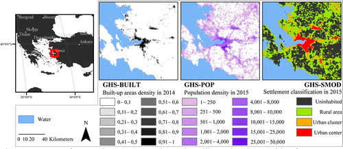
2.1.2. The urban/rural settlements model (GHS-SMOD)

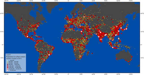
Built-up areas and population density grids are globally consistent and report on human presence independently of administrative divisions. With the availability of built-up areas and population density grids, it became possible to apply the Degree of Urbanisation classification (Dijkstra and Poelman 2014) to the GHSL baseline data and hence to derive a globally consistent delineation of city boundaries at a spatial resolution of 1 km. The Degree of Urbanisation classification is based on a harmonized definition of cities that relies on population thresholds and spatial contiguity rules, which makes it a people-centred definition. This classification discriminates the 1 km populated grid cells in three main classes: (i) ‘urban centres’ (also called cities), (ii) ‘urban clusters’ (also called towns and suburbs), and (ii) ‘rural grid cells’. The applied thresholds are: (i) the population density thresholds on the 1 km cells to identify potential settlements; and (ii) the total population size in a group of contiguous cells that reach the density threshold (i.e. group of cells with a minimal population density) to classify each group of cells as one of the three classes. In the urban/rural Settlements Model (GHS-SMOD) formulation, the ‘urban centres’ class is implemented as a spatial generalization of contiguous population grid cells of 1 km² with a density of at least 1,500 inhabitants per km² or a density of built-up surface >50%, and a minimum total resident population of 50,000 (Figure 1(c)). More details on the classification schema can be found in (Dijkstra and Poelman 2014). In the context of the GHSL, the application of the Degree of Urbanisation classification to the 1 km grids produced a total of 10,323 urban centres in 2015 (Figure 2) (Pesaresi and Freire 2016). These spatially delineated urban centres represent the spatial reference upon which vegetation greenness is assessed and analyzed in the rest of this manuscript.

Figure 2. Urban centres in 2015 according to the GHS-SMOD. Source: Atlas of the Human Planet Pesaresi, Melchiorri, et al. (2016).

2.2. Assessment of greenness from Landsat satellite data

The most conventional and widely used approach for extracting and monitoring vegetation using satellite data is the one relying on spectral indices like the NDVI. The properties of the NDVI can help mitigate a large part of the variations that result from the overall remote-sensing system (e.g. radiometric, spectral, calibration, noise, viewing geometry, and changing atmospheric conditions) (Brown et al. 2006) and that may affect the analysis of changes in vegetation greenness. In this work, the need to extract information on vegetation within the 10,323 urban centres for the period 1990–2014, requires satellite data that offer both high spatial resolution and long-term global coverage. The complete Landsat data archive containing more than 5 million images available in the GEE platform (Gorelick et al. 2017) offers an interesting opportunity to assess greenness at a decametric spatial resolution (30 meters). Moreover, the GEE platform provides a series of pre-calculated products derived from Landsat data. Of interest to this study are the annual greenest pixel TOA reflectance composites. These composites are created from all the scenes in each annual period beginning from the first day of the year and continuing to the last day of the year. All the images from each year are included in the composite, with the pixel with the highest value of the NDVI (i.e. greenest pixel) considered as the composite value. The NDVI is derived from the red:near-infrared reflectance ratio [NDVI = (NIR−RED)/(NIR + RED), where NIR and RED are the amounts of near-infrared and red light, respectively, reflected by the vegetation and captured by the sensor of the satellite]. The formula is based on the fact that vegetation chlorophyll absorbs RED whereas the mesophyll leaf structure scatters NIR. NDVI values thus range from −1 to +1, where negative values correspond to an absence of vegetation (Myneni et al. 1995). Several studies demonstrated the reliability of the NDVI as an indicator to monitor temporal and spatial variations in vegetation as well as health of vegetation cover including urban vegetation (Desnos, Coops, and Hermosilla 2017; Hussein, Kovács, and Tobak 2017). It is also more sensitive to vegetation dynamics, conditions and density compared other vegetation indices like the Enhanced Vegetation Index (EVI) which is more responsive to canopy structural variations, canopy type and architecture (Zhang 2005).

Given our interest in analysing changes in greenness in urban centres in relation to urbanization in the period 1990–2014, for each of the 10,323 urban centres, the average of all greenest pixels falling with the built-up area of the urban centre was calculated for three time intervals centred on the years 1990, 2000 and 2014 as follows: for 1990, the interval spans from 1988-01-01 to 1991-12-30; for 2000, the interval spans from 1999-01-01 to 2002-12-30; for 2014, the interval spans from 2012-01-01 to 2015-12-30. The intervals were chosen in order to match the dates of the Landsat data collections used to derive the multi-temporal built-up areas (GHS-BUILT) (Corbane et al. 2017) and to mitigate inter-annual variability and seasonal anomalies that may affect the greenness change analysis.

The annual greenest pixel TOA reflectance composites needed to cover the three time intervals necessitate the combination of composites from different Landsat sensors, namely Landsat-5 Thematic Mapper (TM), Landsat-7 Enhanced Thematic Mapper (ETM+) and Landsat-8 Operational Land Imager (OLI). Despite the calibration of the sensors, differences in spectral response between them can be expected (Markham and Helder 2012). Regardless of whether TOA or surface reflectance are used to generate NDVI, on average, for vegetated soil and vegetation surfaces (0 ≤ NDVI ≤ 1), the OLI NDVI is greater than the ETM+ NDVI. Statistical functions to transform between the comparable sensor bands and sensor NDVI values are given by Roy et al. (2016) for OLI and ETM+ and by Steven et al. (2003) for ETM+ and TM in order to account for those differences. Hence, to improve the temporal continuity of the greenness values obtained from the three different sensors, we applied the statistical transformations to the NDVI composites as recommended by Roy et al. (2016) and Steven et al. (2003).

These transformations are tailored to NDVI values derived from TOA data and are calculated as follows:(1) $\mathrm{N}\mathrm{D}\mathrm{V}{\mathrm{I}}_{\mathrm{E}\mathrm{T}\mathrm{M}+}=0.002+0.979\mathrm{N}\mathrm{D}\mathrm{V}{\mathrm{I}}_{\mathrm{T}\mathrm{M}}$(1) (2) $\mathrm{N}\mathrm{D}\mathrm{V}{\mathrm{I}}_{\mathrm{O}\mathrm{L}\mathrm{I}}=0.0490+0.9352\mathrm{N}\mathrm{D}\mathrm{V}{\mathrm{I}}_{\mathrm{E}\mathrm{T}\mathrm{M}}$(2)

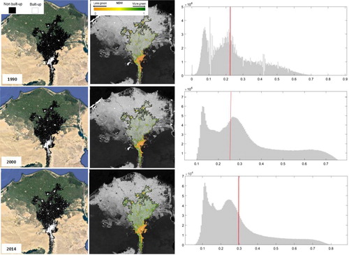
Changes in the built-up areas over time, as observed in the multi-temporal built-up grids of GHS-BUILT, are used to mask the corrected NDVI composites at each time interval (e.g. the non-built-up areas of 1990 are used to mask the NDVI composites for the time interval centred on 1990). Finally, average values of greenness per period are assigned to each urban centre and calculated as an average of all pixels falling within the built-up areas from the NDVI composites. These average values of greenness in the built-up areas of urban centres take into account the urbanization process by considering the changes in the extent of the built-up areas. An illustrative example of the procedure followed for deriving greenness values for 1990, 2000 and 2014 is given in Figure 3 over the urban centre of Cairo in Egypt.

Figure 3. Methodology for calculating the multi-temporal greenness value in the built-up area of an urban centre at a spatial resolution of 30 meters. The example is given for Cairo city with the boundaries of the urban centre depicted in black (middle column). The first column represents the built-up areas for the three periods 1990, 2000 and 2014 derived from the GHSL-BUILT. The middle column represents the annual greenest pixel TOA reflectance composites (NDVI composites) masked by the non-built-up areas of each of the three periods. As a background, the full coverage of the NDVI composite is represented in a greyscale. The last column shows the histograms of the NDVI composites and the average value (red bar) that will be assigned to the urban centre.

2.3. Cross-comparative analysis between TOA-based percentage change of greenness and surface reflectance-based NDVI trends

Despite the use of radiometrically calibrated data for the generation of annual greenest pixel TOA reflectance composites, the quality of the average greenness value derived from the NDVI composites might be affected by a systematic bias due atmospheric contamination (Chander, Markham, and Helder 2009). This could introduce uncertainty in the NDVI-based analysis of the changes in greenness values. To better understand the implications of using non-atmospherically corrected NDVI composites in the analysis of greenness, we propose to compare the changes in average greenness values to trends in vegetation greenness calculated from surface reflectance. The high repeat coverage of Landsat imagery (∼16 days) and the long-term data archive from 1982 to the present make it suitable for assessing long-term vegetation trends. Hence, the Landsat surface reflectance collection available in GEE were used for calculating the NDVI for all cloud free scenes acquired between 1990 and 2014. Despite being very dense in terms of number of available scenes, this collection presents gaps and some quality issues, especially in areas where atmospheric correction is affected by adverse conditions (e.g. hyper-arid, low sun angle conditions, coastal regions). These issues make the surface reflectance-derived NDVI values unsuitable for deriving absolute greenness values at the city level. Still they can be used for the long-term trend analysis. Hence, we applied the Mann-Kendall test to the surface reflectance-derived NDVI values of each pixel falling in the built-up area of an urban centre to verify the existence and direction of significant trends. The Mann-Kendall is a non-parametric method which measures the degree to which a trend is a monotonic increase or decrease over time. It is preferred over the linear regression analysis for estimating trends in NDVI time series due to its robustness against non-normality, missing values and seasonality (Forkel et al. 2013). Kendall's Tau (τ) ranges from -1 to 1 where -1 indicates a consistently decreasing trend while 1 indicates a consistently increasing trend and zero indicates no consistent trend. The Mann-Kendall test produces Z scores to measure the significance of a monotonic trend over time, with a Z value >1.96 representing a significant increasing trend and a Z value <−1.96 indicating a significant decreasing trend (p < 0.05). The analysis was done for the periods 1990–2000 and 2000–2014. The detected trends per pixel were aggregated by calculating the average trend for each urban centre. The mean Kendall Tau (τ) per urban centre is then compared to the percentage change of average greenness values in the same period which is derived from TOA NDVI composites. This allows controlling whether the greenness values available in GEE are appropriate for the assessment of the direction of changes in green spaces over time.

3. Results

3.1. Greenness values in the built-up and non-built-up areas of the urban centres

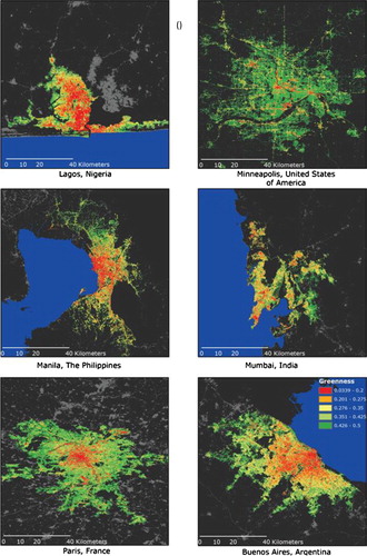
An illustration of the greenness values in the built-up areas derived from NDVI composites is provided in Figure 4. The greenness values are shown here for the time interval centred on 2014 and the six selected cities are displayed here at the same scale and for comparable map extents. The results reflect the variability across cities with each city having varying magnitudes and spatial distribution of greenness. In particular, the assessment of greenness within the built-up areas of Lagos (Nigeria) with a population of 5 million people and Minneapolis (United States of America) with about 0.5 million people, highlights strong differences in the structure and patterns of green vegetation in the two cities. In Minneapolis, pixels with high greenness values are abundant and located inside the built-up area of the urban centre. Whereas in Lagos, the high greenness values are observed in the fringes of the built-up area and the centre of the city is mostly dominated by very low greenness values. Not only there are differences in the values of greenness between the two cities, but also the spatial arrangement of the green spaces is quite different. While green spaces are equally spread in the built-up area of Minneapolis city, the pattern is more compact in Lagos. The differences in the values and patterns of greenness may indicate functional spatial segregation or social inequalities as well as different degrees in population vulnerability as evidenced in several studies (Zhu and Zhang 2008; Wen et al. 2013). In the context of this paper, this example illustrates the interest of studying greenness in the built-up area of the urban centre as a way to better understand the relationship between urbanization and changes in greenness and to clarify the concept of grey-green divide Besides, this continuous data provides an objective metric for the comparison of greenness in cities without the need for hard classification or categorization of the values.

Figure 4. Greenness values in the built-up areas (period 2014) derived from NDVI composites in the urban centres of Minneapolis, Lagos, Manila, Mumbai, Paris and Buenos Aires. The maps are shown at the same scale and cover the same extent.

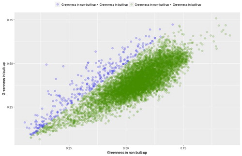
Due to the transformation of vegetated surfaces into impervious surface by urbanization, one might assume that the average greenness values in the built-up areas of the urban centres would never exceed the average greenness values outside the built-up areas. To verify this assumption, average greenness values outside the built-up area of the urban centres were also calculated and compared to those obtained in the built-up areas keeping constant the boundaries of the urban centres. A scatterplot of the greenness values in 2014 calculated in and outside the built-up areas is shown in Figure 5 for the 10,323 urban centres. As expected, most of the urban centres exhibited higher greenness values outside the built-up area than within it. There is a strong linear correlation (Pearson's r = 0.8) between the two measurements suggesting an eventual large scale atmospheric influence and regional climate conditions on the amount of greenness. The most striking observation is the existence of around 400 urban centres where greenness within the built-up areas exceeded that of the surroundings. Most of these urban centres are located in dry and arid regions such as Las Vegas (United States of America), Phoenix (United States of America), Arequipa (Peru), Arrecife (Spain) and Rosarito (Mexico). In such cities, urbanization brings along with it new green spaces by replacing inhabited landscapes with green ‘oasis’ such as golf courses, parks and urban gardens. Such vegetation gains are not always created and managed following the principles of sustainability due to the overexploitation of underground water tables, the excessive use of pesticides and fertilizer and the introduction of invasive species (Gober 2010; Desnos, Coops, and Hermosilla 2017).

Figure 5. Average greenness in the time interval centred on the year 2014 calculated in the built-up and non-built-up areas of the urban centres.

3.2. Relative changes in greenness values in the built-up area

Following the methodology described in Section 2.2, the average greenness values were calculated both in the built-up areas of the urban centres, for the periods 1990, 2000 and 2014. These average values are denoted by:

$\mathrm{A}\mathrm{v}\mathrm{g}.\mathrm{G}\mathrm{r}\mathrm{e}\mathrm{e}{\mathrm{n}}_{\mathrm{B}\mathrm{U},1990},\mathrm{A}\mathrm{v}\mathrm{g}.\mathrm{G}\mathrm{r}\mathrm{e}\mathrm{e}{\mathrm{n}}_{\mathrm{B}\mathrm{U},2000},\mathrm{A}\mathrm{v}\mathrm{g}.\mathrm{G}\mathrm{r}\mathrm{e}\mathrm{e}{\mathrm{n}}_{\mathrm{B}\mathrm{U},2014}$ for the average greenness, in the built-up areas for the periods 1990, 2000 and 2014 respectively.

The relative changes in greenness values in the built-up areas are estimated between 1990–2000 and between 2000–2014 as follows:(3) $P_{\mathrm{c}\mathrm{h}\mathrm{a}\mathrm{n}\mathrm{g}\mathrm{e}\mathrm{\_}1990,2000}=\frac{\mathrm{A}\mathrm{v}\mathrm{g}.\mathrm{G}\mathrm{r}\mathrm{e}\mathrm{e}{\mathrm{n}}_{\mathrm{B}\mathrm{U},2000-\mathrm{A}\mathrm{v}\mathrm{g}.\mathrm{G}\mathrm{r}\mathrm{e}\mathrm{e}{\mathrm{n}}_{\mathrm{B}\mathrm{U},1990}}}{\mathrm{A}\mathrm{v}\mathrm{g}.\mathrm{G}\mathrm{r}\mathrm{e}\mathrm{e}{\mathrm{n}}_{\mathrm{B}\mathrm{U},1990}}\times 100$(3) (4) ${\mathrm{P}}_{\mathrm{c}\mathrm{h}\mathrm{a}\mathrm{n}\mathrm{g}\mathrm{e}\mathrm{\_}2000,2014}=\frac{\mathrm{A}\mathrm{v}\mathrm{g}.\mathrm{G}\mathrm{r}\mathrm{e}\mathrm{e}{\mathrm{n}}_{\mathrm{B}\mathrm{U},2014}-\mathrm{A}\mathrm{v}\mathrm{g}.\mathrm{G}\mathrm{r}\mathrm{e}\mathrm{e}{\mathrm{n}}_{\mathrm{B}\mathrm{U},2000}}{\mathrm{A}\mathrm{v}\mathrm{g}.\mathrm{G}\mathrm{r}\mathrm{e}\mathrm{e}{\mathrm{n}}_{\mathrm{B}\mathrm{U},2000}}\times 100$(4)

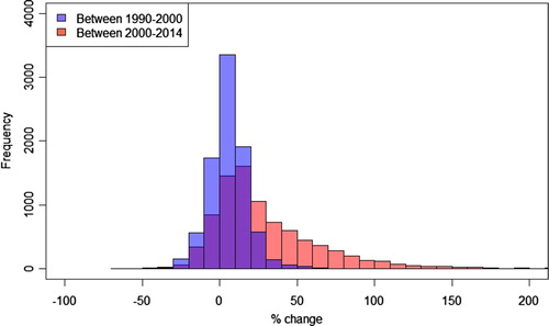
The results for all 10,323 urban centres are summarized in the form of frequency histograms of percentage changes of average greenness values calculated for the two periods (Figure 6). Positive percentages indicate an increase in greenness within the built-up area. The mean and median percentage changes in the time interval 1990–2000 are 30% and 19% respectively. These values decrease to 5.7% and 5.6% in the time interval 2000–2014. The results indicate a general increase in greenness, especially between 1990 and 2000. The greenness continues to increase in the period 2000–2014 though significantly less than in the first period. We also notice a wider range of variation in percentage changes in the period 2000–2014 compared to 1990–2000 and less negative changes (i.e. decreasing greenness). This could be related to wider variations in the changes in the built-up areas within the urban centres in the period 2000–2014 compared to the period 1990–2000 where the built-up areas increased by 15% and 12.5% respectively (Melchiorri et al. submitted).

Figure 6. Frequency histograms of percentage changes of average greenness values in the 10,323 urban centres calculated in the period 1990–2000 and 2000–2014.

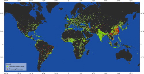
Figure 7 provides an overview of the spatial distribution of greening and ‘browning’ world urban centres for the period 1990–2014. The map depicts a concentration of decreasing greenness in the coastal urban centres of China. In India and European countries, we observe an opposite trend. When observed at a global scale, changes in greenness can be eventually explained by changes in CO₂ concentrations and climate factors. Human influences are more difficult to assess at this scale. As suggested by Schut et al. (2015), on a global scale, land use change is not expected to affect greenness as strongly as the changes in climate or CO₂. Results of Seaquist et al. (2009) suggest that ‘demographic and agricultural pressures in the Sahel are unable to account for differences between simulated and observed vegetation dynamics, even for the most densely populated areas’. Deliberate greening policies for mitigating urban heat islands might also explaining the increasing greenness, however, these policies areas still very localized affecting specific districts or areas within a city (Leal Filho et al. 2017).

Figure 7. Spatial distribution of changes in greenness values for the 10,323 urban centres in the period 1990–2014.

3.3. Comparison of trends in greenness derived from surface reflectance data to changes in greenness calculated from TOA NDVI composites

The percentage change of average greenness values calculated in the previous section is compared to the trends obtained from surface reflectance-derived NDVI with the Mann-Kendall test (see Section 2.3). Only significant greenness trends as identified by Mann-Kendall test are reported here.

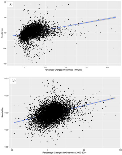
The values of Kendall's Tau are derived from the analysis of NDVI time series calculated on the basis of surface reflectance Landsat data. The trend analysis is performed for the periods 1990–2000 and 2000–2014 separately. The coefficient of determination R² statistics for the two scatter plots in the periods 1990–2000 and 2000–2014 are equal to 0.45 and 0.41 respectively suggesting that the two approaches for assessing of changes in greenness are consistent (Figure 8). Both approaches allocated similar trends for the greenness in the built-up areas for 68% and 65% of the urban centres in the period 1990–2000 and 2000–2014 respectively. These results confirm the suitability of the TOA-based greenness values for the analysis of greenness changes over time.

Figure 8. Scatter plots of Kendall's Tau values vs. percentage changes in greenness in the built-up areas. The Kendall's Tau gives an indication on overall greenness trends in the built-up areas of the urban centres for the periods 1990–2000 (a) and 2000–2014 (b). Kendall's Tau values are derived from the analysis of NDVI time series calculated on the basis of BOA Landsat data.

3.4. Dynamics of urban vegetation in megacities

A close-up analysis of greenness dynamics within the 32 megacities (i.e. cities of at least 10 million inhabitants), identified from to the GHSL population grids (GHS-POP), is shown in Figure 9. The chart represents the three following measures:$\mathrm{A}\mathrm{v}\mathrm{g}.\mathrm{G}\mathrm{r}\mathrm{e}\mathrm{e}{\mathrm{n}}_{\mathrm{B}\mathrm{U},1990},\mathrm{A}\mathrm{v}\mathrm{g}.\mathrm{G}\mathrm{r}\mathrm{e}\mathrm{e}{\mathrm{n}}_{\mathrm{B}\mathrm{U},2000}\mathrm{a}\mathrm{n}\mathrm{d}\mathrm{A}\mathrm{v}\mathrm{g}.\mathrm{G}\mathrm{r}\mathrm{e}\mathrm{e}{\mathrm{n}}_{\mathrm{B}\mathrm{U},2014}.$

Figure 9. Average greenness values in the built-up areas of 32 megacities calculated for the time intervals centred on 1990, 2000 and 2014.

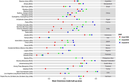
It supports the general analysis at the global level by highlighting an important increase in greenness between 1990 and 2000 in most of the megacities except for Thành Pho Ho Chí Minh in Vietnam and Guangzhou in China. 19 megacities out of 32 (60%) showed also an increase in average greenness in between 2000 and 2014. Megacities where average greenness tends to decrease are essentially located in China. In addition, the megacities of Thành Pho Ho Chí Minh and Los Angeles showed a slight decrease in greenness.

Several physical and socio-economic drivers can affect urban vegetation changes including climate (temperature, precipitation), topography as well as vegetation type. Urban development, changes in population density and urban planning policies are likely to have a more significant influence on urban green spaces than climate and geographic factors (Zhao et al. 2013). Linking social and physical driving factors with the observed vegetation changes is beyond the scope of the paper especially due to regional differences that may require specific analysis at the continental or country levels. However the observed changes can find some elements of explanation in previous research works that analyzed dynamics of greenness in urban areas for selected cities. In a recent study on changes in green spaces in 28 megacities between 2005 and 2015, Huang et al. (2017), found that the percentage of urban green spaces increased significantly between 2005 and 2015. However, five megacities, including Los Angeles, Cairo and Lagos had a slight decrease of the percentage of urban green space. Although a different metric has been used for assessing greenness in urban areas, the results obtained by Huang et al. (2017) are consistent with our findings supporting the generalization of the approach to the global analysis of cities. Some studies attribute the decreasing greenness to droughts, especially in the case of Los Angeles, which experienced medium to severe droughts in the last decade resulting in vegetation stress (Kogan and Guo 2015).

In China, known for having the fastest urbanization in past decades (and this trend is expected to continue in upcoming decades), we observed contrasting trends for vegetation greenness (e.g. decreasing greenness in Beijing and Suzhou and increasing greenness in Shanghai). In China, urban dynamics are vibrant: there are more than 2,100 urban centres, which host 635 million people (+174 million since 1990) and extend over an area exceeding 120,000 km² (+45,000 km² since 1990). Around 800 urban centres doubled their built-up areas between 1990 and 2015. As demonstrated in the statistical analysis of Yang et al. (2014), it is difficult to attribute changes in urban green in Chinese cities to any one of socio-economic or natural factors. The associations between paired variables were seldom unidirectional and linear. In Beijing, Shantou and Suzhou, the urban vegetation showed evident increase between 1990 and 2000. During that same period, Chinese municipal governments have put in efforts in creating new green areas or preserving existing green spaces in conjunction with rapid urbanization in recent years (Zhou et al. 2014). The ‘urban greening’ policies have been found to contribute to the stable or even increasing urban greenness as evidenced in several studies (Zhou and Wang 2011; Zhao et al. 2013).

4. Discussion and conclusion

This research represents advances at several levels over previous studies undertaken in this area. This includes a globally consistent definition of cities using advanced image processing approaches in combination with spatial modelling. Compared to the work of Lu, Coops, and Hermosilla (2016) where a 60-km radius buffer from the city centre was defined for delineating cities or to the use of databases of inconsistent administrative borders (Lu, Coops, and Hermosilla 2016), we adopted a people-based harmonized definition of cities based on the Degree of Urbanisation classification applied to the GHSL data. This approach for delineating urban centres not only allows a more consistent comparison of cities across the world, but it also places the built-up areas and the population densities at the centre of the cities’ definition, both components being potential drivers of changes in vegetation greenness.

In terms of the methodology, the integration of data cubes of high-resolution NDVI composites and trend analysis increased our ability to assess greenness in urban centres and its changes over a period of 25 years. Compared to traditional methods that exploit lower resolution satellite data such as MODIS (250 m) for global scale analysis of greenness, the novelty of the approach presented in this paper lies in the analysis of 25 years of global coverages of high resolution Landsat imagery available in GEE. By combining the Landsat data archive and GEE cloud-computing capabilities, unprecedented monitoring of greenness dynamics was enabled. Unlike most of the studies that rely on the classification of spectral indices (e.g. the NDVI or the Enhanced Vegetation Index (EVI)) or on land use maps (e.g. urban, vegetation, agriculture, etc.), the approach developed in this paper produces a continuous measurement of greenness which was found to be suitable for the analysis of greenness changes over time especially when compared to trends in greenness derived from surface reflectance data This allows overcoming the limitations of the static categorical classifications, which do not represent the dynamics and therefore are insufficient for further statistical analysis given the categorical nature of measurement. The assessment of average greenness values for describing urban vegetation reduces also the problems that may arise from spectral mixing and inferential land cover interpretation that result from the heterogeneity of urban environments (Wentz et al. 2014).

In this research, we focused on examining (i) the greenness values in the built-up areas in comparison to the non-built-up areas, (ii) the changes in greenness values in 10,323 urban centres with a close-up view on world megacities, (iii) the overall trends in greenness in the built-up areas including a geographic distribution of the trends. The results suggest that some general patterns can be observed:

• When assessed at a decametric spatial resolution, the spatial distribution of greenness in the built-up area of the urban centres shows varying temporal and spatial characteristics of urban vegetation both within and across different cities.

• In the large majority of the urban centres, greenness outside the built-up area is greater than inside the built-up area. Some exceptions were identified in arid and desertic landscapes where the gain in urban vegetation is not always considered synonymous to sustainable development.

• Most of the urban centres showed an increase in greenness essentially in the period 1990–2000, despite some regional differences that could be associated to climate factors principally. These findings are in-line with several large scale studies that looked at vegetation trends over the last 25 years and that attributed the general greening to global warming and the phenomena of CO₂ fertilization (Zhu et al. 2016). Environmental and anthropogenic factors likely enhance urban vegetation activity. For example, urban areas tend to have warmer temperatures, greater tropospheric CO₂ concentrations, and higher atmospheric nitrogen depositions, which can promote the plant growth in urban areas (Searle et al. 2012).

• Despite the general greening trend an inspection of absolute average greenness values in megacities showed contrasting trends even within the same country. The differences across cities may be related to a number of environmental as well as social and political factors that are likely to contribute to the observed urban vegetation changes. The combined effects of rapid urbanization and greening policies may sometimes also create contrasting patterns in urban greenness within the same region (Gan et al. 2014).

This work demonstrates the usefulness and potential of GHSL derived datasets combined with time series of high-resolution NDVI composites for conducting in-depth study of the long-term trajectories of urban greenness. Additional insights into the response of urban greenness to urbanization (i.e. urban sprawl or densification) can be gained through the joint analysis of greenness trends and changes in the per capita built-up area derived from the built-up and population grids of the GHSL. Future works will be directed towards a better understanding of the combined effects of urbanization and climate factors on the dynamics of greenness in urban centres (e.g. relationship between greenness and Gross Domestic Product, influence of physical/topographic factors on greenness, relationship between greenness and air temperature and precipitation, and changes in population and built-up areas). This information may provide a valuable reference for urban planners and decision-makers to mitigate urban related environmental and social impacts.

Acknowledgements

The authors are grateful to Guido Lemoine for his advice and support in implementing the algorithms in Google Earth Engine.

Disclosure statement

No potential conflict of interest was reported by the authors.

ORCID

Christina Corbane http://orcid.org/0000-0002-2670-1302

Freire Sergio http://orcid.org/0000-0003-2282-701X

Schiavina Marcello http://orcid.org/0000-0003-3399-3400

References

- Brown, M. E., J. E. Pinzon, K. Didan, J. T. Morisette, and C. J. Tucker. 2006. “Evaluation of the Consistency of Long-Term NDVI Time Series Derived from AVHRR, SPOT-Vegetation, SeaWiFS, MODIS, and Landsat ETM+ Sensors.” IEEE Transactions on Geoscience and Remote Sensing 44 (7): 1787–1793. doi:10.1109/TGRS.2005.860205.
- Chander, Gyanesh, Brian L. Markham, and Dennis L. Helder. 2009. “Summary of Current Radiometric Calibration Coefficients for Landsat MSS, TM, ETM+, and EO-1 ALI Sensors.” Remote Sensing of Environment 113 (5): 893–903. doi:10.1016/j.rse.2009.01.007.
- Chen, Wendy Y., and C. Y. Jim. 2008. “Assessment and Valuation of the Ecosystem Services Provided by Urban Forests.” In Ecology, Planning, and Management of Urban Forests, edited by Margaret M. Carreiro, Yong-Chang Song, and Jianguo Wu, 53–83. New York: Springer New York. doi:10.1007/978-0-387-71425-7_5.
- Corbane, Christina, Martino Pesaresi, Panagiotis Politis, Vasileios Syrris, Aneta J. Florczyk, Pierre Soille, Luca Maffenini, et al. 2017. “Big Earth Data Analytics on Sentinel-1 and Landsat Imagery in Support to Global Human Settlements Mapping.” Big Earth Data 1 (1–2): 118–144. doi:10.1080/20964471.2017.1397899.
- Dallimer, M., Z. Tang, P. R. Bibby, P. Brindley, K. J. Gaston, and Z. G. Davies. 2011. “Temporal Changes in Greenspace in a Highly Urbanized Region.” Biology Letters 7 (5): 763–766. doi:10.1098/rsbl.2011.0025.
- Davies, Richard G., Olga Barbosa, Richard A. Fuller, Jamie Tratalos, Nicholas Burke, Daniel Lewis, Philip H. Warren, and Kevin J. Gaston. 2008. “City-Wide Relationships between Green Spaces, Urban Land Use and Topography.” Urban Ecosystems 11 (3): 269–287. doi:10.1007/s11252-008-0062-y.
- Desnos, Y.-L., N. Coops, and T. Hermosilla. 2017. “Estimating Urban Vegetation Fraction Across 25 Cities in Pan-Pacific Using Landsat Time Series Data.” ISPRS Journal of Photogrammetry and Remote Sensing 126 (April): 11–23. doi:10.1016/j.isprsjprs.2016.12.014.
- Dijkstra, L., and H. Poelman. 2014. “A Harmonised Definition of Cities and Rural Areas: The New Degree of Urbanisation.” Working Papers. Regional Working Paper 2014. http://ec.europa.eu/regional_policy/en/information/publications/working-papers/2014/a-harmonised-definition-of-cities-and-rural-areas-the-new-degree-of-urbanisation.
- Forkel, Matthias, Nuno Carvalhais, Jan Verbesselt, Miguel Mahecha, Christopher Neigh, and Markus Reichstein. 2013. “Trend Change Detection in NDVI Time Series: Effects of Inter-Annual Variability and Methodology.” Remote Sensing 5 (5): 2113–2144. doi:10.3390/rs5052113.
- Freire, Sergio, Thomas Kemper, Martino Pesaresi, Aneta Floczyk, and Vasileios Syrris. 2015. “Combining {GHSL} and {GPW} to Improve Global Population Mapping.” Geoscience and Remote Sensing Symposium (IGARSS), 2015 IEEE International.
- Fuller, R. A., and K. J. Gaston. 2009. “The Scaling of Green Space Coverage in European Cities.” Biology Letters 5 (3): 352–355. doi:10.1098/rsbl.2009.0010.
- Gan, Muye, Jinsong Deng, Xinyu Zheng, Yang Hong, and Ke Wang. 2014. “Monitoring Urban Greenness Dynamics Using Multiple Endmember Spectral Mixture Analysis.” Edited by Clinton N. Jenkins. PLoS ONE 9 (11): e112202. doi:10.1371/journal.pone.0112202.
- Gober, Patricia. 2010. “Desert Urbanization and the Challenges of Water Sustainability.” Current Opinion in Environmental Sustainability 2 (3): 144–150. doi:10.1016/j.cosust.2010.06.006.
- Gorelick, Noel, Matt Hancher, Mike Dixon, Simon Ilyushchenko, David Thau, and Rebecca Moore. 2017. “Google Earth Engine: Planetary-Scale Geospatial Analysis for Everyone.” Remote Sensing of Environment 202: 18–27. doi:10.1016/j.rse.2017.06.031.
- Gutman, G., C. Huang, G. Chander, P. Noojipady, and J. G. Masek. 2013. “Assessment of the NASA-USGS Global Land Survey (GLS) Datasets.” Remote Sensing of Environment 134: 249–265. doi: 10.1016/j.rse.2013.02.026
- Huang, Conghong, Jun Yang, Hui Lu, Huabing Huang, and Le Yu. 2017. “Green Spaces as an Indicator of Urban Health: Evaluating Its Changes in 28 Mega-Cities.” Remote Sensing 9 (12): 1266. doi:10.3390/rs9121266.
- Hussein, Shwan O., Ferenc Kovács, and Zalán Tobak. 2017. “Spatiotemporal Assessment of Vegetation Indices and Land Cover for Erbil City and Its Surrounding Using Modis Imageries.” Journal of Environmental Geography 10 (1–2): 31–39. doi:10.1515/jengeo-2017-0004.
- Ju, Junchang, and Jeffrey G. Masek. 2016. “The Vegetation Greenness Trend in Canada and US Alaska from 1984–2012 Landsat Data.” Remote Sensing of Environment 176 (April): 1–16. doi:10.1016/j.rse.2016.01.001.
- Kogan, Felix, and Wei Guo. 2015. “2006–2015 Mega-Drought in the Western USA and Its Monitoring from Space Data.” Geomatics, Natural Hazards and Risk 6 (8): 651–668. doi:10.1080/19475705.2015.1079265.
- Kumagai, K. 2008. “Analysis of Vegetation Distribution in Urban Areas: Spatial Analysis Approach on a Regional Scale.” International Archives of the Photogrammetry, Remote Sensing and Spatial Information Sciences – ISPRS Archives 37: 101–106. https://www.scopus.com/inward/record.uri?eid=2-s2.0-85012207175&partnerID=40&md5=f9dfa79ea54fa7a62c165ebd14d3f8be.
- Landry, Shawn M., and Jayajit Chakraborty. 2009. “Street Trees and Equity: Evaluating the Spatial Distribution of an Urban Amenity.” Environment and Planning A 41 (11): 2651–2670. doi:10.1068/a41236.
- Leal Filho, Walter, Leyre Echevarria Icaza, Victoria Emanche, and Abul Quasem Al-Amin. 2017. “An Evidence-Based Review of Impacts, Strategies and Tools to Mitigate Urban Heat Islands.” International Journal of Environmental Research and Public Health 14 (12): 1600. doi:10.3390/ijerph14121600.
- Lee, Andrew, Hannah Jordan, and Jason Horsley. 2015. “Value of Urban Green Spaces in Promoting Healthy Living and Wellbeing: Prospects for Planning.” Risk Management and Healthcare Policy 8 (August): 131–137. doi:10.2147/RMHP.S61654.
- Lu, Yuhao, Nicholas C. Coops, and Txomin Hermosilla. 2016. “Regional Assessment of Pan-Pacific Urban Environments Over 25 Years Using Annual Gap Free Landsat Data.” International Journal of Applied Earth Observation and Geoinformation 50 (August): 198–210. doi:10.1016/j.jag.2016.03.013.
- Markham, Brian L., and Dennis L. Helder. 2012. “Forty-Year Calibrated Record of Earth-Reflected Radiance from Landsat: A Review.” Remote Sensing of Environment 122: 30–40. doi: 10.1016/j.rse.2011.06.026
- Melchiorri, M., A. Florczyk, S. Freire, M. Schiavina, M. Pesaresi, and T. Kemper. 2018. “Unveiling 25 Years of Planetary Urbanization with Remote Sensing: Perspectives from the Global Human Settlement Layer.” Remote Sensing 10 (5): 768. doi:10.3390/rs10050768.
- Melchiorri, M., M. Pesaresi, Aneta J. Florczyk, C. Corbane, and T. Kemper. submitted. “Principles and Applications of the Global Human Settlement Layer as Baseline for the Land Use Efficiency Indicator –SDG 11.3.1.” International Journal of Geographical Information Science.
- Myneni, R. B., F. G. Hall, P. J. Sellers, and A. L. Marshak. 1995. “The Interpretation of Spectral Vegetation Indexes.” IEEE Transactions on Geoscience and Remote Sensing 33 (2): 481–486. doi:10.1109/36.377948 doi: 10.1109/TGRS.1995.8746029
- Pesaresi, M., D. Ehrlich, S. Ferri, A. Florczyk, Manuel Carneiro Freire Sergio, S. Halkia, Andreea Julea, T. Kemper, Pierre Soille, and Vasileios Syrris. 2016. Operating Procedure for the Production of the Global Human Settlement Layer from Landsat Data of the Epochs 1975, 1990, 2000, and 2014. Publications Office of the European Union. http://publications.jrc.ec.europa.eu/repository/handle/111111111/40182.
- Pesaresi, M., D. Ehrlich, Aneta J. Florczyk, S. Freire, T. Kemper, A. Julea, P. Soille, and V. Syrris. 2016. GHS Built-up Grid, Derived from Landsat, Multitemporal (1975, 1990, 2000, 2014). (version R2015). European Commission, Joint Research Centre (JRC) [Dataset]. PID. http://data.europa.eu/89h/jrc-ghsl-ghs_built_ldsmt_globe_r2015b.
- Pesaresi, M., and S. Freire. 2016. GHS Settlement Grid, Following the REGIO Model 2014 in Application to GHSL Landsat and CIESIN GPW v4-Multitemporal (1975-1990-2000-2015). (version R2015). European Commission, Joint Research Centre (JRC) [Dataset]. PID. http://data.europa.eu/89h/jrc-ghsl-ghs_smod_pop_globe_r2016a.
- Pesaresi, M., M. Melchiorri, A. Siragusa, and T. Kemper. 2016. Atlas of the Human Planet – Mapping Human Presence on Earth with the Global Human Settlement Layer. JRC103150. Publications Office of the European Union. Luxembourg: European Commission, DG JRC.
- Pesaresi, M., V. Syrris, and A. Julea. 2016. “A New Method for Earth Observation Data Analytics Based on Symbolic Machine Learning.” Remote Sensing 8 (5): 399. doi:10.3390/rs8050399.
- Roy, D., J. Ju, P. Lewis, C. Schaaf, F. Gao, M. Hansen, and E. Lindquist. 2008. “Multi-Temporal MODIS–Landsat Data Fusion for Relative Radiometric Normalization, Gap Filling, and Prediction of Landsat Data.” Remote Sensing of Environment 112 (6): 3112–3130. doi:10.1016/j.rse.2008.03.009.
- Roy, D., V. Kovalskyy, H. K. Zhang, E. F. Vermote, L. Yan, S. S. Kumar, and A. Egorov. 2016. “Characterization of Landsat-7 to Landsat-8 Reflective Wavelength and Normalized Difference Vegetation Index Continuity.” Remote Sensing of Environment 185 (November): 57–70. doi:10.1016/j.rse.2015.12.024.
- Roy, D., M. Wulder, T. Loveland, C. Woodcock, M. Anderson, D. Helder, J. Irons, et al. 2014. “Landsat-8: Science and Product Vision for Terrestrial Global Change Research.” Remote Sensing of Environment 145 (April): 154–172. doi:10.1016/j.rse.2014.02.001.
- Schut, Antonius G. T., Eva Ivits, Jacob G. Conijn, Ben ten Brink, and Rasmus Fensholt. 2015. “Trends in Global Vegetation Activity and Climatic Drivers Indicate a Decoupled Response to Climate Change.” Edited by Lucas C. R. Silva. PLOS ONE 10 (10): e0138013. doi:10.1371/journal.pone.0138013.
- Seaquist, J. W., T. Hickler, L. Eklundh, J. Ardö, and B. W. Heumann. 2009. “Disentangling the Effects of Climate and People on Sahel Vegetation Dynamics.” Biogeosciences (Online) 6 (3): 469–477. doi:10.5194/bg-6-469-2009.
- Searle, S. Y., M. H. Turnbull, N. T. Boelman, W. S. F. Schuster, D. Yakir, and K. L. Griffin. 2012. “Urban Environment of New York City Promotes Growth in Northern Red Oak Seedlings.” Tree Physiology 32 (4): 389–400. doi:10.1093/treephys/tps027.
- Small, Christopher. 2003. “High Spatial Resolution Spectral Mixture Analysis of Urban Reflectance.” Remote Sensing of Environment 88 (1–2): 170–186. doi:10.1016/j.rse.2003.04.008.
- Steven, Michael D., Timothy J. Malthus, Frédéric Baret, Hui Xu, and Mark J. Chopping. 2003. “Intercalibration of Vegetation Indices From Different Sensor Systems.” Remote Sensing of Environment 88 (4): 412–422. doi:10.1016/j.rse.2003.08.010.
- Tan, Puay Yok, James Wang, and Angelia Sia. 2013. “Perspectives on Five Decades of the Urban Greening of Singapore.” Cities (London, England) 32 (June): 24–32. doi:10.1016/j.cities.2013.02.001.
- Townshend, J. R. G., and C. O. Justice. 1988. “Selecting the Spatial Resolution of Satellite Sensors Required for Global Monitoring of Land Transformations.” International Journal of Remote Sensing 9 (2): 187–236. doi:10.1080/01431168808954847.
- United Nations. 2015. Sustainable Development Goals – United Nations. United Nations Sustainable Development. http://www.un.org/sustainabledevelopment/sustainable-development-goals/.
- Walsh, Christopher J., Tim D. Fletcher, and Matthew J. Burns. 2012. “Urban Stormwater Runoff: A New Class of Environmental Flow Problem.” Edited by Jack Anthony Gilbert. PLoS ONE 7 (9): e45814. doi:10.1371/journal.pone.0045814.
- Wen, Ming, Xingyou Zhang, Carmen D. Harris, James B. Holt, and Janet B. Croft. 2013. “Spatial Disparities in the Distribution of Parks and Green Spaces in the USA.” Annals of Behavioral Medicine 45 (S1): 18–27. doi:10.1007/s12160-012-9426-x.
- Wentz, Elizabeth, Sharolyn Anderson, Michail Fragkias, Maik Netzband, Victor Mesev, Soe Myint, Dale Quattrochi, Atiqur Rahman, and Karen Seto. 2014. “Supporting Global Environmental Change Research: A Review of Trends and Knowledge Gaps in Urban Remote Sensing.” Remote Sensing 6 (5): 3879–3905. doi:10.3390/rs6053879.
- Woodcock, C. E., R. Allen, M. Anderson, A. Belward, R. Bindschadler, W. Cohen, F. Gao, et al. 2008. “Free Access to Landsat Imagery.” Science 320 (5879): 1011a–1011a. doi:10.1126/science.320.5879.1011a.
- Yang, Jun, Conghong Huang, Zhiyong Zhang, and Le Wang. 2014. “The Temporal Trend of Urban Green Coverage in Major Chinese Cities between 1990 and 2010.” Urban Forestry & Urban Greening 13 (1): 19–27. doi:10.1016/j.ufug.2013.10.002.
- Yuan, Jiangye. 2017. “Learning Building Extraction in Aerial Scenes with Convolutional Networks.” IEEE Transactions on Pattern Analysis and Machine Intelligence 1–1. doi:10.1109/TPAMI.2017.2750680.
- Zhang, Xiaoyang. 2005. “Monitoring the Response of Vegetation Phenology to Precipitation in Africa by Coupling MODIS and TRMM Instruments.” Journal of Geophysical Research 110 (D12). doi:10.1029/2004JD005263.
- Zhao, Juanjuan, Shengbin Chen, Bo Jiang, Yin Ren, Hua Wang, Jonathan Vause, and Haidong Yu. 2013. “Temporal Trend of Green Space Coverage in China and Its Relationship with Urbanization Over the Last Two Decades.” Science of The Total Environment 442 (January): 455–465. doi:10.1016/j.scitotenv.2012.10.014.
- Zhou, Xiaolu, and Yi-Chen Wang. 2011. “Spatial–Temporal Dynamics of Urban Green Space in Response to Rapid Urbanization and Greening Policies.” Landscape and Urban Planning 100 (3): 268–277. doi:10.1016/j.landurbplan.2010.12.013.
- Zhou, Decheng, Shuqing Zhao, Shuguang Liu, and Liangxia Zhang. 2014. “Spatiotemporal Trends of Terrestrial Vegetation Activity Along the Urban Development Intensity Gradient in China’s 32 Major Cities.” Science of The Total Environment 488–489 (August): 136–145. doi:10.1016/j.scitotenv.2014.04.080.
- Zhu, Z., S. Piao, R. Myneni, M. Huang, Z. Zeng, J. Canadell, P. Ciais, et al. 2016. “Greening of the Earth and Its Drivers.” Nature Climate Change 6 (8): 791–795. doi:10.1038/nclimate3004.
- Zhu, Pengyu, and Yaoqi Zhang. 2008. “Demand for Urban Forests in United States Cities.” Landscape and Urban Planning 84 (3–4): 293–300. doi:10.1016/j.landurbplan.2007.09.005.