Fractional vegetation cover estimation in heterogeneous areas by combining a radiative transfer model and a dynamic vegetation model

ABSTRACT

A fractional vegetation cover (FVC) estimation method incorporating a vegetation growth model and a radiative transfer model was previously developed, which was suitable for FVC estimation in homogeneous areas because the finer-resolution pixels corresponding to one coarse-resolution FVC pixel were all assumed to have the same vegetation growth model. However, this assumption does not hold over heterogeneous areas, meaning that the method cannot be applied to large regions. Therefore, this study proposes a finer spatial resolution FVC estimation method applicable to heterogeneous areas using Landsat 8 Operational Land Imager reflectance data and Global LAnd Surface Satellite (GLASS) FVC product. The FVC product was first decomposed according to the normalized difference vegetation index from the Landsat 8 OLI data. Then, independent dynamic vegetation models were built for each finer-resolution pixel. Finally, the dynamic vegetation model and a radiative transfer model were combined to estimate FVC at the Landsat 8 scale. Validation results indicated that the proposed method (R² = 0.7757, RMSE = 0.0881) performed better than either the previous method (R² = 0.7038, RMSE = 0.1125) or a commonly used method involving look-up table inversions of the PROSAIL model (R² = 0.7457, RMSE = 0.1249).

KEYWORDS:

• Dynamic Bayesian network
• fractional vegetation cover
• global land surface satellite
• radiative transfer model
• dynamic vegetation model

1. Introduction

Fractional vegetation cover (FVC), defined as the fraction of green vegetation in the nadir view, is an important indicator for the assessment and characterization of land surface vegetation conditions (Gitelson et al. 2002; Baret et al. 2013; Camacho et al. 2013). Many fields of research require accurate FVC estimates, because FVC serves as a key parameter in many land surface processes and meteorological models (Hirano, Yasuoka, and Ichinose 2004; Ghulam et al. 2007; Colaizzi et al. 2012). These research areas include drought monitoring, agricultural monitoring, soil erosion assessment, climate change, and the Earth’s energy balance. Therefore, the development of a high-quality land surface FVC estimation method at the regional and global scales is essential.

Remote sensing is the only effective means of generating FVC products at the regional and global scales. Three typical FVC estimation methods using remote-sensing data have been developed and are commonly used, including empirical methods, the pixel un-mixing model, and physical methods. The core of empirical methods is to construct the statistical relationships between FVC and remote sensing data, which include the reflectance of spectral bands and vegetation indices (Carlson and Ripley 1997). For example, a regression model is built using known FVC and paired vegetation index as training data, and then it could be used to estimate FVC based on vegetation index of each pixel (Xiao and Moody 2005). The empirical methods are simple to use, computational efficient and suitable for use in regional scale. However, they have limitations that the statistical relationships are established with training data acquired at specific times and regions, thus are not suitable for transferring to other regions. The pixel un-mixing model is based on the assumption that the photon multiple scattering between the macroscopic materials is relatively inadequate, and the sum of fluxes from the cover types, makes up the fluxes received by the sensor (Jimenez-Munoz et al. 2009; Johnson, Tateishi, and Kobayashi 2012). The proportion of vegetation cover is considered as FVC. However, the endmembers are difficult to determine and extract over large areas because of the complexity of land surface conditions and varied spectral characteristics. The physical methods are based on the inversion of canopy radiative transfer models, which are capable of simulating the physical relationships between the vegetation canopy reflectance and FVC (Kimes et al. 2000; Jia et al. 2015). The physical significance is clear for these models, and they are feasible to be applied for FVC estimation in large scale. However, the physical models are always complex and direct inversion is generally difficult. To simplify the process, the look-up table (LUT) methods or machine learning methods could be adopted. Several large-scale FVC products have been generated using remote-sensing data based on these FVC estimation methods, such as the MEdium Resolution Imaging Spectrometer (MERIS) (Baret et al. 2006), Spinning Enhanced Visible and Infrared Imager (SEVIRI) (Martinez et al. 2007), Change in Land Observational Products from an Ensemble of Satellites (CYCOLPES) (Baret et al. 2007), Geoland2/BioPar version 1 (GEOV1, an improved version of the CYCLOPES FVC product) (Baret et al. 2013), and Global LAnd Surface Satellite (GLASS) FVC products (Liang et al. 2013; Jia et al. 2015). These products contain useful information on the general temporal trends of vegetation change at their respective scales. However, because of the coarse spatial resolution of these products (ranging from 500 m to 6 km), they do not include detailed surface spatial information, and thus the application of these products is limited (Garrigues et al. 2008). Hence, a finer-resolution FVC estimation method is needed.

Vegetation growth characteristics are crucial to describing the process of vegetation growth, estimating vegetation parameters, and discriminating vegetation types (Jia et al. 2014). A previous study improved the accuracy of a coarse-resolution (500 m) FVC estimation method by incorporating vegetation growth characteristics from a dynamic vegetation model into the FVC estimation process (Wang et al. 2016). The dynamic vegetation model was built from field-measured FVC data and the radiative transfer model was integrated using a dynamic Bayesian network (DBN). The validation results suggest that the accuracy of the FVC estimate was improved by incorporating vegetation growth information. Based on this method, a finer spatial resolution (30 m) FVC estimation method was proposed that combined the finer spatial resolution reflectance data and coarse-resolution FVC product (Wang et al. 2017). Due to the lack of field-measured data, the GLASS FVC product was used as the coarse-resolution FVC product to build the regional-scale dynamic vegetation model, and Landsat 7 ETM+ reflectance data were used for the finer spatial resolution reflectance data. The dynamic vegetation model built from one GLASS FVC pixel is considered to represent the corresponding 15 × 15 Landsat pixels, which are assumed to have similar vegetation growth characteristics. However, this method is mainly suitable for a homogeneous region in which the GLASS pixel is pure and it is therefore reasonable to use the dynamic vegetation model built for that pixel for the 15 × 15 Landsat pixels. In heterogeneous areas, using a single dynamic vegetation model may influence the accuracy of the FVC estimate, because there may be multiple Landsat land cover types within a single GLASS pixel. This is mainly caused by different vegetation types or growth conditions occurring within one GLASS pixel. Under these circumstances, the GLASS pixel would no longer be considered as a pure pixel but instead would be considered as a mixed pixel. This becomes a limitation when extending the method to a large area, because most of the Earth’s surface is complex and heterogeneous. It is thus necessary to build a separate dynamic vegetation model for each Landsat pixel to generate accurate FVC estimates using a combined radiative transfer and the dynamic vegetation model.

Therefore, the objective of this study is to develop a finer spatial resolution FVC estimation method for heterogeneous areas by combining the radiative transfer and dynamic vegetation models using the GLASS FVC product and Landsat 8 OLI reflectance data. The accuracy of the dynamic vegetation model built for each pixel of Landsat 8 OLI reflectance data is improved comparing to the previous method. Instead of several finer-resolution pixels sharing one dynamic vegetation model built by the corresponding GLASS pixel, each Landsat 8 OLI pixel has its own unique dynamic vegetation model. The proposed method is validated over a vegetation transitional region with complex land cover types in northern China and is compared to a similar previously developed method (Wang et al. 2017) and a commonly used method involving look-up table (LUT) inversions of the PROSAIL model (Ding and Zheng 2016).

2. Study area and data

2.1. Study area

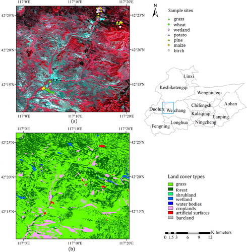
The selected study area is in Weichang county, Hebei Province, North China, and belongs to the semi-humid and semi-dry climate region of the temperate zone (Figure 1). The average annual temperature in the study area ranges from −1.4 °C to 4.7°C and total annual precipitation is approximately 500 mm. The study area contains a complex distribution of many different land types, including broad-leaf and coniferous forest, both high and low FVC grassland, low FVC cropland, and residential areas (Jia et al. 2016). The land cover distributions are shown in Figure 1(b) with a land cover map from the global 30 m land cover dataset (GlobeLand30) in the year 2010 (Chen, Yifang, and Songnian 2015). The study area is a typical heterogeneous area with diverse types of vegetation, and can be used for validating the FVC estimation result using the proposed method.

Figure 1. The geographic location of the study area (the blue rectangle in the administrative map). The images on the left are the study area shown by the Landsat 8 OLI image with standard false color composition (a) and the land cover map from the global 30 m land cover dataset (GlobeLand30) in the year 2010 (b). The points with different colors and shapes on the Landsat 8 image (a) are the locations of the sample sites.

2.2. Landsat 8 OLI reflectance data

Landsat 8 OLI surface reflectance data (Path 123, Row 031) from 2014 for day of year (DOY) 87–295 were selected as the finer-resolution remote-sensing observations. Heavy cloud contaminated Landsat 8 OLI images (cloud cover more than 80% over the study area) were pre-screened and not used in this study (Table 1). The Landsat 8 OLI sensor consists of nine spectral bands with 30 m spatial resolution (15 m for the panchromatic band) with a time interval of 16 days (Ali, Darvishzadeh, and Skidmore 2017). The main bands used in this study were bands 4 (Red) and 5 (NIR). These images were downloaded from the U.S. Geological Survey’s (USGS) EarthExplorer (https://earthexplorer.usgs.gov/).

Table 1. The main data used in this study.

Data type	DOY	Temporal resolution	Spatial resolution
Landsat 8 OLI reflectance	71/87/103/119/135/199/231/247/279/295	16 days	30 m
GLASS FVC	73/89/105/121/137/201/233/249/281/297	8 days	500 m
Field measured FVC	204/205/206/207/208	--	--

*DOY: Day of Year. Heavy cloud contaminated Landsat 8 OLI images (DOY 151/167/183/215/263) were not used in this study.

2.3. GLASS FVC product

The GLASS FVC product was chosen as the coarse-resolution FVC product in this study. The GLASS FVC product was generated from MODIS surface reflectance data (MOD09A1) at a resolution of 500 m every 8 days using machine learning algorithms based on the training samples generated from global distributed Landsat Thematic Mapper (TM) and Enhanced Thematic Mapper plus (ETM+) data (Jia et al. 2015). The general regression neural networks (GRNNs) method was firstly used to generate GLASS FVC product using MODIS data. However, due to the unsatisfactory computational efficiency of GRNNs method, four machine learning methods were assessed to find a suitable one and the multivariate adaptive regression splines (MARS) method was determined as the final method for generating GLASS FVC because of its satisfactory computational efficiency and accuracy (Yang et al. 2016; Jia et al. 2018). The validation results showed satisfactory accuracy and spatial and temporal continuity of the GLASS FVC product (Jia et al. 2015). Therefore, the GLASS FVC was a suitable choice as the coarse resolution FVC product in this study. The GLASS FVC data were re-projected from the sinusoidal projection to the Universal Transverse Mercator (UTM) projection using the MODIS Reprojection Tools (MRT) for consistency with the Landsat 8 OLI reflectance data.

2.4. Field-measured FVC data

A ground survey was conducted to obtain field-measured FVC data. Several sample sites were selected, based on the ground survey conditions from July 23, 2014 to July 27, 2014. Basic information about the sample sites is shown in Table 2. The size of each site was approximately 30 m × 30 m. The sample sites, which had a variety of growth conditions, contained the following vegetation types: grass, maize, wheat, potato, wetland, pine, and white birch. The geographic coordinates at the central point of each sample site were measured with a hand-held global positioning system receiver that had a positioning accuracy of approximately ±3 m. Five photographs were taken at each sampling site, one at the center of the square and one each at the mid-point of the diagonal between the center point and each corner. For low-growing vegetation (such as grass and crops), the photographs were taken from the nadir approximately two meters above the ground at each survey point. For tall trees such as pine and white birch, photographs were taken facing up and facing down to capture the tree canopy and the low near-ground vegetation, respectively. To eliminate distortion effects in the digital images, the edges of the photographs were cut. Then the FVC of each edge-cut photograph was extracted using an automatic shadow-resistant algorithm in the Internationale de L'Eclairage (CIE) L*a*b* color space (SHAR-LABFVC) (Song et al. 2015). For pine trees, the maximum likelihood classifier (Duda and Hart 1973) was used instead of the automatic FVC extraction method, as the latter was sometimes biased low due to interruptions by arborous branches and unidentified dark leaves. In forest regions, the field FVC was calculated using the following equation:(1) $\mathrm{F}\mathrm{V}\mathrm{C}={\mathrm{f}}_{\mathrm{u}\mathrm{p}}+(1-{\mathrm{f}}_{\mathrm{u}\mathrm{p}})\times {\mathrm{f}}_{\mathrm{d}\mathrm{o}\mathrm{w}\mathrm{n}}$(1) where f_up and f_down are FVC values extracted from the upward-facing and downward-facing photographs, respectively.

Table 2. Basic information on the sample sites.

Site number	Latitude(°)	Longitude(°)	Land cover	Sampling date
1	42.2374	117.0719	Grass	2014/7/23
2	42.2391	117.0716	Grass	2014/7/23
3	42.2392	117.081	Grass	2014/7/25
4	42.2335	117.0944	Grass	2014/7/25
5	42.2297	117.0932	Grass	2014/7/25
6	42.2317	117.089	Grass	2014/7/25
7	42.2333	117.0854	Grass	2014/7/25
8	42.2361	117.0781	Grass	2014/7/25
9	42.2344	117.0827	Grass	2014/7/25
10	42.2408	117.0647	Maize	2014/7/24
11	42.2395	117.0631	Maize	2014/7/24
12	42.2405	117.0626	Maize	2014/7/24
13	42.2545	117.0844	Wheat	2014/7/25
14	42.2533	117.0858	Potato	2014/7/25
15	42.2514	117.086	Potato	2014/7/25
16	42.4307	117.2403	Wetland	2014/7/26
17	42.4269	117.2464	Wetland	2014/7/26
18	42.4318	117.2447	Wetland	2014/7/26
19	42.4135	117.2411	Pine	2014/7/24
20	42.4264	117.2496	Pine	2014/7/26
21	42.4298	117.252	Pine	2014/7/26
22	42.4328	117.2492	Pine	2014/7/26
23	42.4337	117.2369	Pine	2014/7/26
24	42.4192	117.2429	Pine	2014/7/26
25	42.3992	117.317	Pine	2014/7/27
26	42.3975	117.3111	Pine	2014/7/27
27	42.3994	117.3163	Pine	2014/7/27
28	42.3979	117.3041	Pine	2014/7/27
29	42.3973	117.308	Pine	2014/7/27
30	42.399	117.3041	Pine	2014/7/26
31	42.3987	117.317	Pine	2014/7/26
32	42.4237	117.2403	White birch	2014/7/26
33	42.3979	117.3154	White birch	2014/7/27
34	42.3882	117.3128	White birch	2014/7/27
35	42.3975	117.3165	White birch	2014/7/26

3. Methods

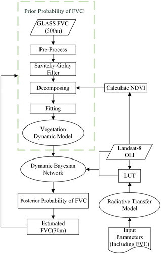
A flowchart of the proposed finer spatial resolution FVC estimation method is shown in Figure 2. First, the GLASS FVC product is decomposed so that it has the same spatial resolution as the Landsat 8 OLI reflectance data. The normalized difference vegetation index (NDVI) of Landsat 8 OLI pixels was used to address the problem of heterogeneity when decomposing the GLASS FVC product. Then the time series of the decomposed GLASS FVC data are used to build the dynamic vegetation model for each Landsat 8 OLI pixel. Finally, the dynamic vegetation model is combined with the radiative transfer model to estimate FVC using the DBN.

Figure 2. Flowchart of the proposed method based on the radiative transfer model and the dynamic vegetation model.

3.1. GLASS FVC decomposition method for finer resolution background FVC

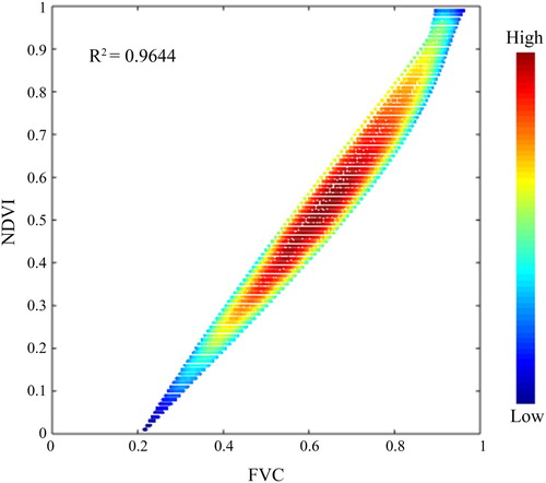
To build an independent dynamic vegetation model for each Landsat 8 OLI pixel, a method for the decomposition of the GLASS FVC data was developed, allowing background FVC values to be obtained for each Landsat 8 OLI pixel in this study. Assuming that the coarse-resolution FVC pixel is a linear combination of the FVC of the land-cover components, all the finer-resolution reflectance data pixels corresponding to one pixel of coarse-resolution FVC data can be regarded as endmembers of the coarse-resolution FVC pixel. The weight of each endmember in the linear combination can be determined by their growth conditions. NDVI is a widely used vegetation index for describing vegetation growth conditions and a candidate variable for the weight of endmembers. To demonstrate the approximate linear relationship between FVC and NDVI, NDVI values are obtained from PROSAIL model simulations (in which NDVI values are calculated from the simulated red and NIR reflectance data) and the scatter plots between FVC and NDVI values are shown in Figure 3. FVC and NDVI are well-correlated (R² = 0.9644), supporting the use of NDVI for the weight of the endmembers in this study.

Figure 3. Scatter plots between FVC and the corresponding NDVI based on PROSAIL simulations, which demonstrates the approximate linear relationship between FVC and NDVI.

Based on the assumption that the GLASS FVC pixels are linear combinations of the FVC of the land-cover components, the GLASS FVC data can be decomposed so that they have the same spatial resolution as the Landsat 8 OLI reflectance data. Figure 4 shows the approach used for the decomposition of the GLASS FVC pixels. The GLASS FVC time series data are first smoothed using a Savitzky–Golay filter (Chen et al. 2004). Then, the GLASS pixel is resampled to a 30 m × 30 m spatial resolution to match the Landsat 8 OLI reflectance data using a nearest-neighbor sampling algorithm. Meanwhile, the NDVI of the Landsat 8 image was calculated using red and NIR bands’ reflectance for each pixel. Then a moving window matching the size of the GLASS FVC pixel is used to determine the value of the decomposed result of the central pixel of the moving window as follows:(2) $\mathrm{F}\mathrm{V}{\mathrm{C}}_{\mathrm{k}}=\frac{\mathrm{N}\mathrm{D}\mathrm{V}{\mathrm{I}}_{\mathrm{k}}{\sum }_{\mathrm{i}=1}^{\mathrm{M}}\mathrm{f}\mathrm{v}{\mathrm{c}}_{\mathrm{i}}}{{\sum }_{\mathrm{i}=1}^{\mathrm{M}}\mathrm{N}\mathrm{D}\mathrm{V}{\mathrm{I}}_{\mathrm{i}}}$(2) where M is the total number of endmembers within a moving window (set to the number of Landsat 8 OLI pixels within one GLASS pixel), fvc_i denotes the resampled FVC value of an endmember within the moving window from the coarse-resolution FVC product, NDVI_i is the NDVI value of the finer-resolution pixel, FVC_k represents the decomposed FVC value of the central pixel of the moving window, and NDVI_k is the NDVI value of that pixel. NDVI_k is calculated from the finer-resolution reflectance pixel that serves as the weight of the central pixel in the decomposing process. Finally, the moving window moves to finish determining the decomposed FVC of every Landsat 8 OLI pixel.

Figure 4. Diagram of the GLASS FVC decomposition approach, which allocates background FVC from GLASS FVC pixels to every Landsat 8 pixel based on its NDVI.

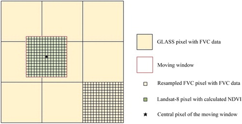
Decomposing the GLASS FVC pixel for the Landsat 8 OLI pixels can improve the accuracy of the background FVC over heterogeneous areas, allowing a more accurate dynamic vegetation model to be obtained. The decomposition procedure will have less influence on the background FVC in homogeneous landscapes, because the NDVI of finer spatial resolution reflectance pixels within a coarse-resolution FVC pixel are very similar within a homogeneous area.

3.2. Dynamic vegetation model

A dynamic vegetation model was used as a dynamic process model that could describe the dynamic change of FVC. Two kinds of dynamic vegetation models have been developed to describe the vegetation growth process: models with clear physical mechanism describing the intrinsic properties of vegetation growth (Ritchie 1985; Boogaard 1998; Jones et al. 2003) and models that rely on statistical analyses of time series data (Gregorczyk 1998; Bindraban 1999; Wu et al. 2003). The use of the first kind is limited by its complexity, as it requires a large number of input parameters, although the biomechanism of the plant is relatively clear in the model. In the second kind, observational time series data, including field-measured data or remote-sensing products, are used to construct a statistical dynamic vegetation model, which is easy to implement and has acceptable performance. For these reasons, this study employs the second kind of model. Specifically, the modified Verhulst logistic equation (Lin et al. 2003) was selected to construct the dynamic vegetation model as follows:(3) $\mathrm{F}\mathrm{V}\mathrm{C}=\frac{\mathrm{d}}{1+\exp (\mathrm{a}\ast {\mathrm{t}}^2+\mathrm{b}\ast \mathrm{t}+\mathrm{c})}$(3) where a, b, c, and d are the coefficients, and t is DOY.

For each Landsat 8 OLI pixel, the Universal Global Optimization (UGO) algorithm was used to identify the best initial value for the model parameters and the Levenberg-Marquardt (LM) algorithm was used to fit the model parameters to the decomposed GLASS FVC data. The LM algorithm combines the steepest descent and the Gauss–Newton methods and is widely used to address nonlinear least-squares problems (Lourakis 2005). For each fitting process, an initial value was provided for the coefficients and the iteration was stopped when the sum of squares reached a minimum.

3.3. Radiative transfer model

In this study, the simulated vegetation canopy reflectance was obtained from the coupled PROSPECT leaf optical properties model and the SAIL canopy bidirectional reflectance model, which is referred to as the PROSAIL model. Due to its simplicity, accuracy and general robustness, the PROSAIL model has become one of the most popular model to develop vegetation parameter estimation methods (Jacquemoud et al. 2009). The PROSPECT model assumes a leaf as one or several absorbing thin, rough-surface plates that produce isotropic scattering. It simulates directional-hemispherical reflectance and transmittance by describing leaf optical properties at the leaf level (Jacquemoud and Baret 1990; Jacquemoud et al. 2000). The PROSPECT model generates leaf reflectance and transmittance with a spectral range of 400–2500 nm, using input parameters including leaf structure parameter (N), leaf chlorophyll a + b concentration (${\mathrm{C}}_{\mathrm{a}\mathrm{b}}$), dry matter content (${\mathrm{C}}_{\mathrm{m}}$), water content (${\mathrm{C}}_{\mathrm{w}}$), carotenoid content (${\mathrm{C}}_{\mathrm{a}\mathrm{r}}$), and brown pigment content (${\mathrm{C}}_{\mathrm{b}\mathrm{r}\mathrm{o}\mathrm{w}\mathrm{n}}$) (Jacquemoud et al. 2009). Then the output of PROSPECT is used as input to the SAIL model. The SAIL model, which is a canopy bidirectional reflectance distribution function model, assumes that canopy is horizontal and infinitely extended (Verhoef 1984). Its input parameters include leaf reflectance, leaf transmittance, leaf area index (LAI), average leaf angle inclination (ALA), hot-spot parameter (Hot), viewing zenith angle (VZA), relative azimuth angle (RAZ), and soil reflectance.

The PROSAIL input parameters are shown in Table 3. LAI was converted from reasonable range FVC (Table 3) using the classical gap fraction relationship between LAI and ALA under the assumption of a turbid medium, which can be expressed as follows:(4) $\mathrm{P}\mathrm{o}\left(\theta \right)=\exp \left(-\frac{\mathrm{G}(\theta ,\mathrm{L}\mathrm{I}\mathrm{D}\mathrm{F})}{\cos \left(\theta \right)}\right)\ast \mathrm{L}\mathrm{A}\mathrm{I}$(4) (5) $\mathrm{F}\mathrm{V}\mathrm{C}=1-\mathrm{P}\mathrm{o}(0^{\mathrm{o}})$(5) where Po(θ) is the gap fraction in the direction θ (θ equals 0° at the nadir view), G(θ, LIDF) is the projection function, and LIDF is the leaf inclination distribution function characterized by the ALA and ellipsoidal distribution. In addition, soil reflectance (G) was simulated using Price’s model, which constructs high-spectral-resolution soil reflectance with four spectral eigenvectors (Price 1990). The remaining input parameters were fixed to a single value or a logical range, mainly according to the Leaf Optical Properties Experiment 93 (LOPEX’93) database (Feret et al. 2008). The solar zenith, viewing zenith, and relative azimuth angles can be acquired from the metadata file of the Landsat 8 OLI scenes. The high-resolution canopy reflectance computed using PROSAIL was then resampled to simulate the Landsat 8 observations in the red and near infrared (NIR) bands based on the relative spectral response profiles. Then, the simulated red and NIR band reflectance and their corresponding input variables in different permutations and combinations were saved in the LUTs. The LUT were used to generate the 2-D conditional probability distributions (CPDs), which describe the probability of capturing each discrete red and NIR reflectance value by the OLI sensor at a certain FVC value in a step of its range for a Landsat 8 OLI pixel. The CPDs were saved in conditional probability tables (CPTs) with discrete reflectance values along one dimension and discrete FVC values along the other.

Table 3. The input variables of the PROSAIL model.

Parameters	Value range	Step	Units
FVC	0.01–0.99	0.01	–
ALA	30–60	10	°
N	2	–	–
Cab	30–60	10	µg/cm^2
Cm	0.005	–	g/cm^2
Car	4.4	–	µg/cm^2
Cw	0.01	–	cm
Cbrown	0–0.05	0.05	–
Hot	0.1	–	–
SZA	25–60	5	°
VZA	0	–	°
RAZ	135–160	5	°

*ALA: average leaf inclination angle; N: leaf structure parameter; C_ab: leaf chlorophyll a + b concentration; C_m: dry matter content; C_ar: carotenoid content; C_w: water content; C_brown: brown pigment content; Hot: hot-spot parameter; SZA: solar zenith angle; VZA: viewing zenith angle; RAZ: relative azimuth angle.

3.4. Dynamic Bayesian network for finer spatial resolution FVC estimation

The DBN is used to combine all the information from the Landsat 8 OLI reflectance data, dynamic vegetation model, and radiative transfer model to obtain optimal FVC estimates with a finer spatial resolution. The main structure of the DBN (further details may be found in Ref. Wang et al. 2016) can be described as follows:(6) $\mathrm{P}\left(\mathrm{F}\mathrm{V}{\mathrm{C}}_{\mathrm{T}}\right|\mathrm{Re}{\mathrm{f}}_{\mathrm{T}})=\frac{\mathrm{P}\left(\mathrm{r}\mathrm{e}{\mathrm{f}}_{\mathrm{T}}\right|\mathrm{F}\mathrm{V}{\mathrm{C}}_{\mathrm{T}}){\sum }_{\mathrm{F}\mathrm{V}{\mathrm{C}}_{\mathrm{T}-1}}\mathrm{P}\left(\mathrm{F}\mathrm{V}{\mathrm{C}}_{\mathrm{T}}\right|\mathrm{F}\mathrm{V}{\mathrm{C}}_{\mathrm{T}-1}\left)\mathrm{P}\right(\mathrm{F}\mathrm{V}{\mathrm{C}}_{\mathrm{T}-1}\left|\mathrm{Re}{\mathrm{f}}_{\mathrm{T}-1}\right)}{{\sum }_{\mathrm{F}\mathrm{V}{\mathrm{C}}_{\mathrm{T}}}\mathrm{P}\left(\mathrm{r}\mathrm{e}{\mathrm{f}}_{\mathrm{T}}\right|\mathrm{F}\mathrm{V}{\mathrm{C}}_{\mathrm{T}}\left)\mathrm{P}\right(\mathrm{F}\mathrm{V}{\mathrm{C}}_{\mathrm{T}}\left|\mathrm{Re}{\mathrm{f}}_{\mathrm{T}-1}\right)}$(6) where P(FVC_T|Ref_T) is the state estimate of FVC at time T, Ref_T represents the reflectance data, FVC_T donates the FVC value, and P(ref_T|FVC_T) is the likelihood probability of the dynamic process and is calculated in the following manner. First, the probabilities of observed reflectance are calculated based on the assumption that the remote-sensing data uncertainties obey the Gaussian distribution. Then, the calculated probabilities located in discrete intervals (the variable FVC is discretized from continuously distributed into discrete intervals, and each discrete interval is set to 0.05 such that there are 20 intervals for an FVC range of 0 to 1) are combined with the CPTs generated by the simulations of the PROSAIL model. P(FVC_T|FVC_T−1) is the state transition probability obtained from the dynamic vegetation model. P(FVC_T−1|Ref_T−1) can be obtained by the DBN at time T−1. Finally, the minimum mean square error (MMSE) estimation method is used to calculate the optimal FVC value from P(FVC_T|Ref_T) at the current time.

In this study, the error in remote-sensing observations and the dynamic vegetation model were both assumed to obey the Gaussian distribution. The normal cumulative distribution function was used to calculate the likelihood probabilities and the state transition probability. Finally, because the posterior probability also meets the Gaussian distribution (Wikle and Berliner 2007; Qu and Zhang 2009), a 90% confidence interval of the estimated FVC value was calculated using the normal cumulative distribution function to illustrate the associated uncertainties of FVC estimates for each pixel using the DBN method.

4. Results

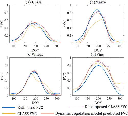
Time series of the FVC estimates were generated from the Landsat 8 OLI data and the dynamic vegetation model constructed from the decomposed GLASS FVC data. Figure 5(a1–a3) shows the estimated finer spatial resolution FVC images on DOY 135, 199, and 231, which represent low, high, and medium vegetation growth conditions, respectively. The textural information is rich, and the characteristics of the small land patches are successfully captured. In addition, the results show a trend of vegetation growth in the time series. The northern and eastern parts of the region are mainly in mountainous areas covered by forests, whereas the remaining parts are plains with grassland and cropland. The FVC changes rapidly in the plain regions, whereas the FVC variation is comparably slow in the mountainous areas, because some of the coniferous forests are evergreen and lack of obvious seasonality. For the visual interpretation of the estimated FVC results, the GLASS FVC on DOY 137, 201, and 233 are also shown in Figure 5 (b1–b3). The FVC estimates using the proposed method are practically consistent with the GLASS FVC on the corresponding dates. In addition, to determine whether the temporal trajectories of the estimated FVC being conform to the vegetation growth characteristics, four typical sites were selected to compare the time-series GLASS FVC, decomposed GLASS FVC, the FVC predicted by the dynamic vegetation model, and the FVC estimated using the proposed method (Figure 6). The temporal trajectories of the FVC estimation are conform to the vegetation growth characteristics.

Figure 5. FVC estimated using the proposed method at DOY 135 (a1), DOY 199 (a2), and DOY 231 (a3). GLASS FVC images at DOY 137 (b1), DOY 201 (b2) and DOY 233 (b3).

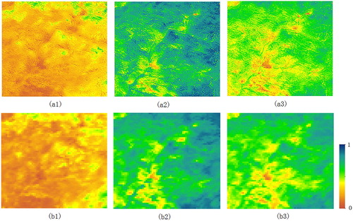
Figure 6. Comparison of the temporal trajectories of GLASS FVC, decomposed GLASS FVC, the FVC predicted by the dynamic vegetation model, and the FVC estimated using the proposed method.

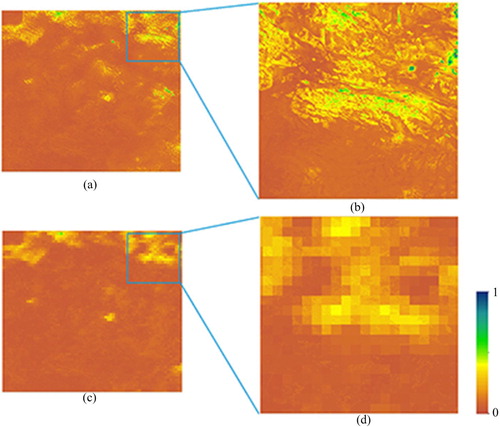
In order to assess the performance of the proposed method over heterogeneous areas, the FVC estimation result obtained by the previous method (Wang et al. 2017), in which coarse FVC data were not decomposed, was used for comparison. Figure 7 shows the FVC estimation result on DOY 103 using both methods. It is clear that the FVC estimation from the proposed method reflects more spatial detailed information and shows much more heterogeneity and granularity, better reflecting the heterogeneity of natural environments, while the result from the previous method has obvious ‘mosaicking’ and some spatial details are missing. This is due to the presence of mixed pixels over these heterogeneous landscapes, as mentioned in section 3.1. The decomposition approach helps reducing errors in each finer-resolution pixel and presenting reasonable FVC estimates as determined by visual comparison.

Figure 7. The FVC estimation on DOY 103 using the proposed method (a) and the previous method (c). The right column presents close-up images of a forested area for the proposed method (b) and the previous method (d).

To quantitatively evaluate the performance of the proposed method, a direct validation comparison between the performance of the proposed method and the previous method (Wang et al. 2017) was conducted using the field-measured FVC data collected during DOY 204–208. The cubic spine interpolation method was used to match the time of the resultant FVC and field survey data, where the average and maximum gap in time between the two is 7.5 days and 9 days, respectively. Figure 8 shows the relationship between the FVC estimates and the field measured data. The FVC estimates using the proposed method achieved satisfactory performance (R² = 0.7757, RMSE = 0.0881), and fell close to the 1:1 line. The FVC estimates of the pine sites are distributed around 85%, which is reasonable due to the similar forest canopy structure of these planted trees in the study area. In addition, the maize and potato sites were in their growth peak and their FVC was relatively high. The FVC of the grass sites was lower than the aforementioned vegetation types owing to their thin leaves. In addition, the performance of FVC estimates using the previous method is inferior to the results of the proposed method. The proposed method has a slightly better fit in the lower FVCs while this appear opposite in the previous method, and the previous method may be reaching an asymptote at around 0.8. Therefore, these results indicate the proposed method is reliable for FVC estimation in heterogeneous areas.

Figure 8. Scatter plots of the field-measured FVC and estimated FVC using the proposed method (a) and the previous method (b). Error bars indicates a 90% confidence interval of the FVC estimation at each point.

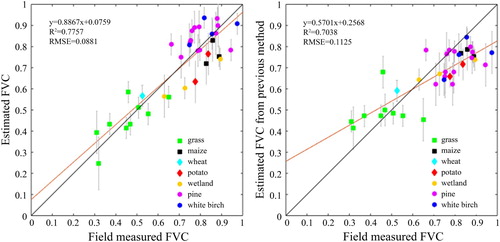
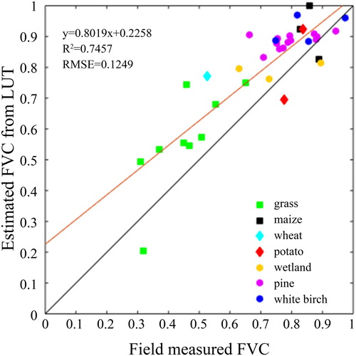
To further compare the performance between the proposed method and currently existing FVC estimation methods, the commonly used LUT method was also conducted for comparison. The LUT method, which uses inversions of the PROSAIL model (Ding and Zheng 2016) from Landsat 8 OLI reflectance data, was also validated by field-measured FVC data (Figure 9). Because the uncertainty of the LUT method is difficult to quantify, no error bars are shown in Figure 9. The validation results of the LUT method (R² = 0.7457, RMSE = 0.1249) were inferior to the proposed method. The LUT method FVC estimates were biased high, as evidenced by most points falling above the 1:1 line. This comparison further indicates the reliability of the proposed method.

Figure 9. Scatter plots of the field-measured FVC and estimated FVC using the LUT method from the PROSAIL model.

5. Discussion

This study proposed a method to overcome the difficulties in estimating finer spatial resolution FVC over heterogeneous areas. Instead of several Landsat 8 OLI pixels sharing one dynamic vegetation model built by the FVC data of their corresponding GLASS FVC pixel, the proposed method built a dynamic vegetation model for each Landsat 8 OLI pixel by decomposing the GLASS FVC product. This method uses multiple information including the Landsat 8 OLI reflectance data, GLASS FVC product, dynamic vegetation model and radiative transfer model, takes the characteristics of heterogeneous areas into consideration, and is shown to be reliable for regional FVC estimation. It also has the advantage of requiring neither human interaction nor many of the parameters required by the empirical method and pixel un-mixing models. The decomposition approach reduces the mixed-pixel problem in dynamic vegetation modeling and improves the accuracy of finer spatial resolution FVC estimates at a region scale with complex land-cover types. Furthermore, the proposed method is simple and easily constructed. It not only produced good results in reducing the mixing phenomenon within the mixed GLASS FVC pixels but was also highly efficient. This method is suitable for both homogeneous and heterogeneous landscapes, thus widening the scope of its potential applications.

Both this study and its predecessor take advantage of the DBN, which is a probabilistic framework that combines a process model (in this study, a dynamic vegetation model) with observations. However, the present study assumes that the GLASS FVC pixels were mixed and composed of a linear combination of FVC values from Landsat 8 pixels, whereas the previous study considered the GLASS FVC pixels to be pure pixels. In this study, NDVI is used to weight the endmembers of the linear combination. Other vegetation indices that have the potential to represent growth conditions should also be investigated in future. Furthermore, the previous method (Wang et al. 2017) is only suitable for FVC estimation in a small region with certain types of land cover (mainly uniform croplands). This becomes a limitation when trying to apply the method for FVC estimation on a larger scale. By taking into consideration heterogeneous landscapes, the decomposition approach presented here generates more precise background FVC values for finer spatial resolution pixels, allowing a more accurate dynamic vegetation model to be built. The proposed method can now be applied for FVC estimation in extensive regions.

In this study, validation of the FVC estimates was mainly conducted by scatter plots. Although various vegetation types and vegetation conditions were considered, the field measurements were mainly conducted on DOY 204–208, 2014. More time series field measurements are needed to further assess the accuracy of this method. In addition, within-canopy upward-facing photographs were used to estimate tree FVC. This may cause underestimation for dense tree canopies, where the upper leaves may be shielded by branches and trunks. This limitation could potentially be overcome in future studies by using an unmanned aircraft system to take photographs from the nadir above the tall tree canopies.

The proposed method is demonstrated to successfully estimate FVC at the regional scale. When applied to a larger scale, the land surface conditions are even more complex. A more accurate and computationally efficient dynamic vegetation model building method should be developed. In addition, the FVC value is related to the vegetation growth characteristics which are influenced by the climatic conditions such as temperature or precipitation. Therefore, when applying the method to a larger or the global scale, using semi-empirical dynamic vegetation model with input parameters including climatic factors might improve the description about vegetation growth characteristics under different climate conditions and potentially improving the FVC estimation accuracy. The proposed method was used for FVC estimation at the Landsat resolution. It is also suitable for other finer spatial resolution data for FVC estimation such as HJ-1, Sentinel-2, GF-1, and CBERS. Furthermore, the Landsat (or similar) high-resolution satellite data usually have low temporal resolution and their quality is also often influenced by cloud contaminations, which bring difficulties on high temporal resolution FVC estimation at large scales. Jointly using other similar or higher spatial resolution data (such as finer spatial resolution data mentioned above) to promote the amount of temporal reflectance observation may overcome this issue and will be the further work of this study. In addition, interpolation method based on the dynamic vegetation model may also be adopted to obtain high temporal resolution FVC estimations.

6. Conclusion

A fractional vegetation cover estimation method for heterogeneous areas that combines a radiative transfer model and a dynamic vegetation model using a DBN was proposed in this study. Unlike previous methods, the proposed method does not use a single dynamic vegetation model to represent several finer spatial resolution pixels corresponding to one coarse-resolution FVC pixel, which is only reasonable for homogeneous regions. Instead, the coarse-resolution FVC pixel is decomposed to build a dynamic vegetation model for each finer-resolution pixel by accounting for the differences among these pixels in heterogeneous areas. The Landsat 8 OLI reflectance data and the GLASS FVC product were used to evaluate the proposed method in a heterogeneous region with various land-cover types. The validation results showed that the proposed method could effectively address heterogeneous landscapes and could achieve satisfactory FVC estimates. Future work will focus on further assessment of the proposed method based on more field measured data as well as applying it for high-spatial-resolution FVC estimation at regional scales.

Acknowledgements

This work was supported by the National Natural Science Foundation of China under Grant 41671332 and Grant 41571422, and in part by the National Key Research and Development Program of China under Grant 2016YFA0600103. The authors thank Dr. X. Mu from Beijing Normal University for providing part of the field reference data. The authors would also like to thank the anonymous reviewers and the editor for the constructive comments and suggestions, all of which have led to great improvements in the presentation of this article.

Disclosure statement

No potential conflict of interest was reported by the authors.

Additional information

Funding

This work was supported by the National Natural Science Foundation of China under [Grant 41671332 and Grant 41571422], and in part by the National Key Research and Development Program of China under [Grant 2016YFA0600103].

References

- Ali, A. M., R. Darvishzadeh, and A. K. Skidmore. 2017. “Retrieval of Specific Leaf Area from Landsat-8 Surface Reflectance Data Using Statistical and Physical Models.” IEEE Journal of Selected Topics in Applied Earth Observations and Remote Sensing 10 (8): 3529–3536. doi: 10.1109/JSTARS.2017.2690623
- Baret, F., O. Hagolle, B. Geiger, P. Bicheron, B. Miras, M. Huc, B. Berthelot, et al. 2007. “LAI, fAPAR and FCover CYCLOPES Global Products Derived from Vegetation.” Remote Sensing of Environment 110 (3): 275–286. doi: 10.1016/j.rse.2007.02.018
- Baret, F., K. Pavageau, D. Béal, M. Weiss, B. Berthelot, and P. Regner. 2006. Algorithm Theoretical Basis Document for MERIS top of Atmosphere Land Products (TOA_VEG). Avignon: INRA-CSE.
- Baret, F., M. Weiss, R. Lacaze, F. Camacho, H. Makhmara, P. Pacholcyzk, and B. Smets. 2013. “GEOV1: LAI and FAPAR Essential Climate Variables and FCOVER Global Time Series Capitalizing Over Existing Products. Part1: Principles of Development and Production.” Remote Sensing of Environment 137: 299–309. doi: 10.1016/j.rse.2012.12.027
- Bindraban, P. 1999. “Impact of Canopy Nitrogen Profile in Wheat on Growth.” Field Crops Research 63 (1): 63–77. doi: 10.1016/S0378-4290(99)00030-1
- Boogaard, H. 1998. User’s Guide for the WOFOST 7.1 Crop Growth Simulation Model and WOFOST Control Center 1.5 Technical Document 52 DLO Vinand Staring Centre. Wageningen: Wageningen University & Research.
- Camacho, F., J. Cernicharo, R. Lacaze, F. Baret, and M. Weiss. 2013. “GEOV1: LAI, FAPAR Essential Climate Variables and FCOVER Global Time Series Capitalizing Over Existing Products. Part 2: Validation and Intercomparison with Reference Products.” Remote Sensing of Environment 137: 310–329. doi: 10.1016/j.rse.2013.02.030
- Carlson, T. N., and D. A. Ripley. 1997. “On the Relation between NDVI, Fractional Vegetation Cover, and Leaf Area Index.” Remote Sensing of Environment 62 (3): 241–252. doi: 10.1016/S0034-4257(97)00104-1
- Chen, J., P. Jönsson, M. Tamura, Z. Gu, B. Matsushita, and L. Eklundh. 2004. “A Simple Method for Reconstructing a High-Quality NDVI Time-Series Data set Based on the Savitzky–Golay Filter.” Remote Sensing of Environment 91 (3–4): 332–344. doi: 10.1016/j.rse.2004.03.014
- Chen, J., B. Yifang, and L. Songnian. 2015. “China: Open Access to Earth Land-Cover Map.” Nature 514 (7523): 434.
- Colaizzi, P. D., W. P. Kustas, M. C. Anderson, N. Agam, J. A. Tolk, S. R. Evett, T. A. Howell, Gowda, P. H., and O’Shaughnessy, S. A., 2012. “Two-source Energy Balance Model Estimates of Evapotranspiration Using Component and Composite Surface Temperatures.” Advances in Water Resources 50: 134–151. doi: 10.1016/j.advwatres.2012.06.004
- Ding, Y., and X. Zheng. 2016. “Comparison of Fractional Vegetation Cover Estimations Using Dimidiate Pixel Models and Look-up Table Inversions of the PROSAIL Model From Landsat 8 OLI Data.” Journal of Applied Remote Sensing 10 (3): 036022. doi: 10.1117/1.JRS.10.036022
- Duda, R. O., and P. E. Hart. 1973. Pattern Classification and Scene Analysis. New York: Wiley.
- Feret, J.-B., C. François, G. P. Asner, A. A. Gitelson, R. E. Martin, L. P. R. Bidel, S. L. Ustin, le Maire, G., and S. Jacquemoud. 2008. “PROSPECT-4 and 5: Advances in the Leaf Optical Properties Model Separating Photosynthetic Pigments.” Remote Sensing of Environment 112 (6): 3030–3043. doi: 10.1016/j.rse.2008.02.012
- Garrigues, S., D. Allard, F. Baret, and J. Morisette. 2008. “Multivariate Quantification of Landscape Spatial Heterogeneity Using Variogram Models.” Remote Sensing of Environment 112 (1): 216–230. doi: 10.1016/j.rse.2007.04.017
- Ghulam, A., Q. Qin, T. Teyip, and Z.-L. Li. 2007. “Modified Perpendicular Drought Index (MPDI): a Real-Time Drought Monitoring Method.” ISPRS Journal of Photogrammetry and Remote Sensing 62 (2): 150–164. doi: 10.1016/j.isprsjprs.2007.03.002
- Gitelson, A. A., Y. J. Kaufman, R. Stark, and D. Rundquist. 2002. “Novel Algorithms for Remote Estimation of Vegetation Fraction.” Remote Sensing of Environment 80 (1): 76–87. doi: 10.1016/S0034-4257(01)00289-9
- Gregorczyk, A. 1998. “Richards Plant Growth Model.” Journal of Agronomy and Crop Science 181 (4): 243–247. doi: 10.1111/j.1439-037X.1998.tb00424.x
- Hirano, Y., Y. Yasuoka, and T. Ichinose. 2004. “Urban Climate Simulation by Incorporating Satellite-Derived Vegetation Cover Distribution Into a Mesoscale Meteorological Model.” Theoretical and Applied Climatology 79 (3–4): 175–184. doi: 10.1007/s00704-004-0069-0
- Jacquemoud, S., C. Bacour, H. Poilvé, and J. P. Frangi. 2000. “Comparison of Four Radiative Transfer Models to Simulate Plant Canopies Reflectance Direct and Inverse Mode.” Remote Sensing of Environment 74 (3): 471–481. doi: 10.1016/S0034-4257(00)00139-5
- Jacquemoud, S., and F. Baret. 1990. “Prospect: A Model of Leaf Optical Properties Spectra.” Remote Sensing of Environment 34 (2): 75–91. doi: 10.1016/0034-4257(90)90100-Z
- Jacquemoud, S., W. Verhoef, F. Baret, C. Bacour, P. J. Zarco-Tejada, G. P. Asner, C. François, and S. L. Ustin. 2009. “PROSPECT+SAIL Models: A Review of use for Vegetation Characterization.” Remote Sensing of Environment 113: S56–S66. doi: 10.1016/j.rse.2008.01.026
- Jia, K., S. Liang, X. Gu, F. Baret, X. Wei, X. Wang, Y. Yao, L. Yang, and Y. Li. 2016. “Fractional Vegetation Cover Estimation Algorithm for Chinese GF-1 Wide Field View Data.” Remote Sensing of Environment 177: 184–191. doi: 10.1016/j.rse.2016.02.019
- Jia, K., S. Liang, S. Liu, Y. Li, Z. Xiao, Y. Yao, B. Jiang, et al. 2015. “Global Land Surface Fractional Vegetation Cover Estimation Using General Regression Neural Networks From MODIS Surface Reflectance.” IEEE Transactions on Geoscience and Remote Sensing 53 (9): 4787–4796. doi: 10.1109/TGRS.2015.2409563
- Jia, K., S. Liang, X. Wei, Y. Yao, Y. Su, B. Jiang, and X. Wang. 2014. “Land Cover Classification of Landsat Data with Phenological Features Extracted From Time Series MODIS NDVI Data.” Remote Sensing 6 (11): 11518–11532. doi: 10.3390/rs61111518
- Jia, K., S. Liang, X. Wei, Y. Yao, L. Yang, X. Zhang, and D. Liu. 2018. “Validation of Global LAnd Surface Satellite (GLASS) Fractional Vegetation Cover Product From MODIS Data in an Agricultural Region.” Remote Sensing Letters 9 (9): 847–856. doi: 10.1080/2150704X.2018.1484958
- Jimenez-Munoz, J. C., J. A. Sobrino, A. Plaza, L. Guanter, J. Moreno, and P. Martinez. 2009. “Comparison between Fractional Vegetation Cover Retrievals from Vegetation Indices and Spectral Mixture Analysis: Case Study of PROBA/CHRIS Data Over an Agricultural Area.” Sensors (Basel) 9 (2): 768–793. doi: 10.3390/s90200768
- Johnson, B., R. Tateishi, and T. Kobayashi. 2012. “Remote Sensing of Fractional Green Vegetation Cover Using Spatially-Interpolated Endmembers.” Remote Sensing 4 (12): 2619–2634. doi: 10.3390/rs4092619
- Jones, J. W., G. Hoogenboom, C. H. Porter, K. J. Boote, W. D. Batchelor, L. A. Hunt, P. W. Wilkens, et al. 2003. “The DSSAT Cropping System Model.” European Journal of Agronomy 18 (3–4): 235–265. doi: 10.1016/S1161-0301(02)00107-7
- Kimes, D. S., Y. Knyazikhin, J. L. Privette, A. A. Abuelgasim, and F. Gao. 2000. “Inversion Methods for Physically-Based Models.” Remote Sensing Reviews 18 (2–4): 381–439. doi: 10.1080/02757250009532396
- Liang, S., X. Zhao, S. Liu, W. Yuan, X. Cheng, Z. Xiao, X. Zhang, et al. 2013. “A Long-Term Global LAnd Surface Satellite (GLASS) Data-set for Environmental Studies.” International Journal of Digital Earth 6 (sup1): 5–33. doi: 10.1080/17538947.2013.805262
- Lin, Z. H., Y. Q. Xiang, M. O. Xing-Guo, L. I. Jun, and L. Wang. 2003. “Normalized Leaf Area Index Model for Summer Maize.” Chinese Journal of Eco-Agriculture 11 (4): 69–72.
- Lourakis, M. I. 2005. “A Brief Description of the Levenberg-Marquardt Algorithm Implemented by Levmar.” Foundation of Research and Technology 4 (1): 1–6.
- Martinez, B., A. Verger, F. J. Garcia-Haro, M. Gilabert, and J. Melia. 2007. “Procedure for the Regional Scale Mapping of FVC and LAI Over Land Degradated Areas in the DeSurvey Project.” In Geoscience and Remote Sensing Symposium, 2007. IGARSS 2007. IEEE International, IEEE.
- Price, J. C. 1990. “On the Information Content of Soil Reflectance Spectra.” Remote Sensing of Environment 33 (2): 113–121. doi: 10.1016/0034-4257(90)90037-M
- Qu, Y., and Y. Zhang. 2009. “Fusing Near-Infrared Reflectance Spectrum and Dynamic Model to Estimate Vegetation Structural Parameters.” International Congress on Image and Signal Processing, Tianjin.
- Ritchie, J., and S. Otter. 1985. “Description and Performance of CERES Wheat: A User-Oriented Wheat Yield Model.” In ARS Wheat Yield Project, 159–175. Springfield, MO: National Technical Information Service.
- Song, W., X. Mu, G. Yan, and S. Huang. 2015. “Extracting the Green Fractional Vegetation Cover From Digital Images Using a Shadow-Resistant Algorithm (SHAR-LABFVC).” Remote Sensing 7 (8): 10425–10443. doi: 10.3390/rs70810425
- Verhoef, W. 1984. “Light Scattering by Leaf Layers with Application to Canopy Reflectance Modeling: The SAIL Model.” Remote Sensing of Environment 16 (2): 125–141. doi: 10.1016/0034-4257(84)90057-9
- Wang, X., K. Jia, S. Liang, Q. Li, X. Wei, Y. Yao, X. Zhang, and Y. Tu. 2017. “Estimating Fractional Vegetation Cover from Landsat-7 ETM+ Reflectance Data Based on a Coupled Radiative Transfer and Crop Growth Model.” IEEE Transactions on Geoscience and Remote Sensing 55 (10): 5539–5546. doi: 10.1109/TGRS.2017.2709803
- Wang, X., K. Jia, S. Liang, and Y. Zhang. 2016. “Fractional Vegetation Cover Estimation Method Through Dynamic Bayesian Network Combining Radiative Transfer Model and Crop Growth Model.” IEEE Transactions on Geoscience and Remote Sensing 54 (12): 7442–7450. doi: 10.1109/TGRS.2016.2604007
- Wikle, C. K., and L. M. Berliner. 2007. “A Bayesian Tutorial for Data Assimilation.” Physica D: Nonlinear Phenomena 230 (1–2): 1–16. doi: 10.1016/j.physd.2006.09.017
- Wu, R., C. X. Ma, W. Zhao, and G. Casella. 2003. “Functional Mapping for Quantitative Trait Loci Governing Growth Rates: a Parametric Model.” Physiological Genomics 14 (3): 241–249. doi: 10.1152/physiolgenomics.00013.2003
- Xiao, J., and A. Moody. 2005. “A Comparison of Methods for Estimating Fractional Green Vegetation Cover Within a Desert-to-Upland Transition Zone in Central New Mexico, USA.” Remote Sensing of Environment 98 (2–3): 237–250. doi: 10.1016/j.rse.2005.07.011
- Yang, L., K. Jia, S. Liang, J. Liu, and X. Wang. 2016. “Comparison of Four Machine Learning Methods for Generating the GLASS Fractional Vegetation Cover Product from MODIS Data.” Remote Sensing 8 (8): 682. doi: 10.3390/rs8080682