Hybrid model to optimize object-based land cover classification by meta-heuristic algorithm: an example for supporting urban management in Ha Noi, Viet Nam

ABSTRACT

This study proposed a novel object-based hybrid classification model named GMNN that combines Grasshopper Optimization Algorithm (GOA) and the multiple-class Neural network (MNN) for urban pattern detection in Hanoi, Vietnam. Four bands of SPOT 7 image and derivable NDVI, NDWI were used to generate image segments with associated attributes by PCI Geomatics software. These segments were classified into four urban surface types (namely water, impervious surface, vegetation and bare soil) by the proposed model. Alternatively, three training and validation datasets of different sizes were used to verify the robustness of this model. For all tests, the overall accuracies of the classification were approximately 87%, and the Area under Receiver Operating Characteristic curves for each land cover type was 0.97. Also, the performance of this model was examined by comparing several statistical indicators with common benchmark classifiers. The results showed that GMNN out-performed established methods in all comparable indicators. These results suggested that our hybrid model was successfully deployed in the study area and could be used as an alternative classification method for urban land cover studies. In a broader sense, classification methods will be enriched with the active and fast-growing contribution of metaheuristic algorithms.

KEYWORDS:

• Urban
• remote sensing
• object-based classification
• neural network
• grasshopper optimization algorithm

1. Introduction

Urban management activities require an accurate spatial/temporal database and an effective management strategy to minimize adverse effects (Herold and Sawada 2012; Jonkman and Dawson 2012). In these database, land cover maps are very important as they provide preliminary information about the spatial variation of surface types. Therefore, adequate detection of urban landscape plays a considerable role in the proper handling of certain types of land covers. It also helps the decision-making process in coping various environmental hazards, such as excessive surface runoff and urban flooding. The identification of land cover types can significantly contribute to the efficient management and reduction of damages to the settlement, agriculture, and livelihood by avoiding construction and developments in hazard-prone areas.

Methods for land cover classification methods can be divided into two branches, which are pixel-based and object-based classification. The latter has significantly grown in the last several years with the rapid emergence of high spatial resolution, i.e. (smaller than 4 m). Applications of this approach can be found in many studies that have shown the superior performance of object-based classification over the traditional pixel-based approach (Duro, Franklin, and Dubé 2012; Myint et al. 2011). In fact, object-based classification is sensitive to landscape morphology and is found to be a robust method in an urban study where the human-made structure is present at a high density (Qian et al. 2015).

Typically, the conventional object-based classification process comprises of image segmentation and classification of segments based on predefined class properties. Depending on specific locations, three typical parameters, which are scale, compactness, and shape are be defined, mainly by user’s experiences (Qian et al. 2015). The definition of those parameters controls how pixels or existing objects are grouped and ultimately impacts the overall accuracy of classification tasks. In addition to built-in algorithms (rule-based method) in popular image analysis packages (W. Zhou and Troy 2008), machine learning has been increasingly used to fine tune the parameters of classifiers. This approach could be found in (Hamedianfar et al. 2014) with the C4.5 algorithm in urban mapping from hyperspectral images, or the applications of Support Vector Machine (SVM) with high resolution images in review papers of (Mountrakis, Im, and Ogole 2011) and (Petropoulos, Kalaitzidis, and Prasad Vadrevu 2012). Another common technique could also be found in (Belgiu and Drăguţ 2016; Gong, Im, and Mountrakis 2011) where random forest and variances of neural network (including deep learning) significantly improved classification accuracies of the regular object-based method. Some methods also introduced and evaluated ensemble techniques to strengthen weak classifiers as in (Chan and Paelinckx 2008). From the literature, it could be seen that few studies employed the power of metaheuristic algorithms in optimizing image classification methods, except for some recent works of (Dou et al. 2015). Recently, researchers have enriched optimization libraries with fast-developed algorithms, mainly by nature-inspired algorithms. In fact, no algorithm is capable of solving all optimization problems and the examinations of new algorithms to specific applications are therefore necessary.

This study posed several questions on how meta-heuristic algorithms could be used for fine tuning classifiers to improve classification performance and how the variation in sizes of training data could impact classification overall accuracy and individual accuracies for each of four surface type extractions. To partly answer these questions, this study proposed a novel hybrid model, named GMNN that employs Grasshopper Optimization Algorithm (GOA) to optimize parameters of the multiple-class neural network (MNN) for urban pattern detection. GOA was chosen because despite being successfully tested against benchmarked theoretical functions, the algorithm has yet been examined in a real application.

Hanoi, the capital of Vietnam was selected as the subject of a case study because of its complex surface morphology and patterns of land cover types. GMNN was run with different training and validation data sizes, and the classified outputs were compared to several benchmarked classifiers such as Support Vector Machine (SVM), Decision Tree (DT) (Qian et al. 2015), and MNN optimized by two other new algorithms such as Grey Wolf Optimization (GWO), Biogeography-based Optimization (BBO) through conventional statistical indicators. Throughout the experiments, PCI Geomatics (Trial mode) was used for image segmentation and feature extraction; Matlab was used for modeling; QGIS was used for map visualization. Detail description of the procedure and results are in the following sections, including Data and method in the second part, Results, and discussion in the third and Conclusion in the final section.

2. Data and methods

2.1 Study area

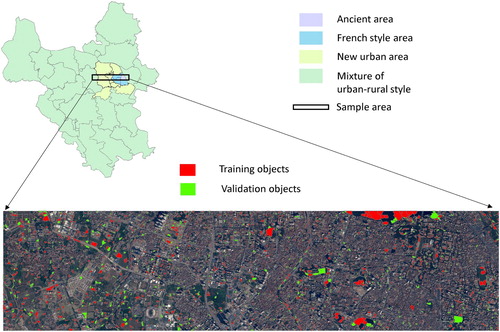
Hanoi, the capital city of Viet Nam, currently experiences a high rate of urbanization, which was a consequence of the decision to expand the city administrative boundary in 2008. The rapid urbanization was associated with the conversion of large areas of agricultural land into residential/public land and was accompanied with rapid inhabitation (Nguyen et al. 2016). The study area is special as it comprises of (1) a central area including ancient and French-style districts; (2) a new urban area with high-rise building in the western part where impervious surfaces are dominant with mixed patches of open space; (3) the remaining areas are a mixture of urban-rural styles in outskirt of the city, in which bare soil and agricultural are commonly found (Figure 1).

Figure 1. Study area.

2.2 Remotely sensed data and preprocessing

High spatial resolution images, such as Worldview, Ikonos, Quickbird, SPOT … are the usual sources of data for object-based classification studies. Indeed, the selection of satellite images is much dependent on the availability of data and dates of capture. For this study, we used SPOT 7 image captured on 28 December 2016 with the spectral specification described in (Table 1). In sequential order, the image pre-processing includes converting the Digital number into surface reflectance and rectifying image into local map projection. In this study, we used COST (COSine Theta) method to determine 1% of dark objects in the image and to calculate surface reflectance by subtracting radiance differences. The image was then rectified to global UTM projection (WGS84). Since SPOT 7 was characterized by one Panchromatic and four spectral bands as described in (Table 1), the fusion technique as introduced by (Yuri 2002) was used to generate multiple spectral bands with a 1.5 m spatial resolution. The fusion process started with standardizing histograms of Pan and MS bands to minimize spectral errors, and the output image was calculated by using (Equation 1)(1) $S=\sum _{i=1}^N{\omega }_{i}M{S}_{i\uparrow }$(1) where S is the synthesized image, N is the total number of MS bands, ${\omega }_i$ is a scalar weight, $M{S}_{i\uparrow }$ is the up-scaled i-th MS band. ${\omega }_i$ is determined by minimizing the least square error of ||P-S|| (Yuri 2002). After that, fussed bands are generated by using(2) $F_i=\frac{P}{S}M{S}_{i\uparrow }$(2) where F_i is the ith band in the fused (pan-sharpened) image, P is the PAN image, S is the synthesized image, and $M{S}_{i\uparrow }$ is the up-scaled i-th MS band (Yuri 2002).

Table 1. SPOT 7 specification.

	Bands	Spectral range	Spatial resolution
Original image	Blue	0.455 µm – 0.525 µm	6.0 m
	Green	0.530 µm – 0.590 µm	6.0 m
	Red	0.625 µm – 0.695 µm	6.0 m
	Near-Infrared	0.760 µm – 0.890 µm	6.0 m
	Panchromatic	0.450 µm – 0.745 µm	1.5 m
Fusion	(B,G,R,NIR)		1.5 m

2.3 Image segmentation

After the enlargement of the administrative border in 2008, the study area is described as having complex urban morphology and livelihoods. We selected a horizontally stretched subset, covering all four types of land covers to construct training and validation datasets. For this study, aiming at classifying urban cover pattern to support urban management, we proposed four separable classes namely (1) impervious surfaces; (2) vegetation; (3) water; and (4) bare soil. These four classes are typically generalized pattern in an urban area and were also investigated in previous studies (Qian et al. 2015). The quantification of those surface covers has a significant contribution to urban management, such as flood management. Indeed, shadows in the high-spatial resolution are inevitable. They were also classified into a separate class by using the method described in (Weiqi Zhou and Troy 2009) and were manually assigned a label into one of the four mentioned classes.

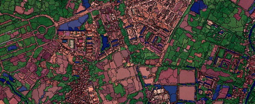
The object-based classification started with image segmentation procedure. Although there is some guidance to select criteria for the segmentation process, it is truly generalizable and normally subjected to the specific geographic condition. The image segments are essentially groups of adjacent pixels that have similar characteristics regarding spectral and spatial information (Yuri 2002). Normally, image segmentation is based on the determination of scale, shape, and compactness. Of all, the scale parameter is the most important parameter that directly affects the size of each image object. The quality of image classification depends directly on the quality of the image segmentation. An optimal selection of the three parameters is achieved through a trial-error approach, based on the nature of the study area, to generate meaningful segments. The smaller the scale, the smaller segments are generated and it might lead to fragmented but more homogenous segmentation. After several trials, to avoid mixture of objects, we defined the scale level at 30 as objects were visually homogenous and seem fit with typical pattern arrangement of Hanoi. Embedded procedure in PCI Geomatics (2017 Trial mode) was used to generate segments with a definition for scale at 30, shape at 0.75, and compactness at 0.5. Four bands of SPOT 7 including Blue, Green, Red, NIR and derivable NDVI, NDMI were used as input images. Specifically, NDVI was calculated by (NIR – Red)/(NIR + Red), and NDWI was calculated by using equation (Green – NIR)/(Green + NIR). Totally, the procedure generated approximately 54.000 objects and (Figure 2) showed a subset of segmentation result.

Figure 2. Image segmentation at Scale: 30, Shape: 0.75, and Compactness: 0.5.

Another crucial step is feature selection that aims to find an optimal collection of predictor variables. Feature attributes generated in the previous step including channel and geometrical statistics such as area, perimeters, pixel value … for each segment and for each band. Indeed, proper selection of attributes is subjected to geographic variations of the study area and spatial resolution of input images (Qian et al. 2015). In fact, each commercial and open-source software generates different attributes associated with image segments, such as default Mean value, brightness, Mean-difference-to-super-object, etc. in eCognition or with custom measurements in OpenCV (Wieland and Pittore 2014). Sometimes, these attributes were further processed to filter redundant variables and to reduce dimensionality by using embedded algorithms in commercial image processing software or by using machine learning techniques (Dou et al. 2015; Hamedianfar et al. 2014). In this study, we used all attributes that were generated from the image processing procedure using PCI Geomatics. Detail description of variables was presented in (Table 2)

Table 2. Predictor variables extracted from image segmentation.

ID	Object features	Number of bands	Description
1.	Min pixel value	6	Min pixel values for each of 6 bands
2.	Max pixel value	6	Max pixel values for each of 6 bands
3.	Mean pixel value	6	Mean pixel values for each of 6 bands
4.	Standard deviation	6	Standard deviation of pixel value
5.	Min_PP	6	Mean pure pixel
6.	Max_PP	6	Max pure pixel
7.	Mean_PP	6	Mean pure pixel
8.	Standard deviation _PP	6	Standard deviation of pure pixel
9.	Circular	1	Circular
10.	Compactness	1	Compactness
11.	Elongation	1	Elongation
12.	Rectangular	1	Rectangular
Total predictor variables		52

2.4 Multiple-classes neural network

The neural network is one of the most common methods, among other conventional machine learning techniques, for solving either binary or multiple-classes classification problems (Gong, Im, and Mountrakis 2011). For this study, neural topology is presented in (Figure 3). The Input layer consisted of 52 predictor variables as described in (Table 2), N hidden neurons in the middle, and four output classes, as mentioned in the previous section, in the output layer. The determination of N value would be discussed in the next section.(3) $\mathrm{R}\mathrm{M}\mathrm{S}\mathrm{E}=\sqrt{\frac{1}{4\ast n}\sum _1^n{\left(\mathrm{o}\mathrm{b}\mathrm{s}\mathrm{e}\mathrm{r}\mathrm{v}\mathrm{e}{\mathrm{d}}_{ij}-\mathrm{c}\mathrm{a}\mathrm{l}\mathrm{c}\mathrm{u}\mathrm{l}\mathrm{a}\mathrm{t}\mathrm{e}{\mathrm{d}}_{ij}\right)}^2}$(3) where i = 1 : n (number of samples); j = 1 : 4 (number of classes); observed_ij is observed value of sample_i for class_j and calculated_ij is value generated by model of sample_i for class_j. Four classes are described in section 2.3

Figure 3. Neural network topology.

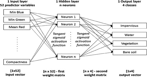
Mathematically the network was [1 × 52] (input vector) -> [n × 52] (first weight matrix) -> [n × 4] (the second weight matrix) -> [1 × 4] (output classes). Also, Tangent sigmoid activation function was used in each node. Root Mean Square Error (RMSE) was used as fitness function and was calculated by differences between output values and observed values as described in (Equation 3).

2.5 Grasshopper optimization algorithm

Metaheuristic algorithm is a fast growing and active research area to catch up with changes of the nature of problems, particularly with increasing data size. Of which, GOA is a relatively new swarm intelligence algorithm that mathematically mimics the behaviors of grasshopper movement. It was first introduced by (Saremi, Mirjalili, and Lewis 2017) to solve either constrained and unconstrained problems (Abhishek G Neve 2017). The performance of this algorithm was examined against several popular algorithms for solving 13 benchmark test functions. Simply, GOA procedure can be described as follows:

Grasshoppers move in a swarm and the relative positions between two insects are defined in a comfort zone (the boundary where repulsion and attraction forces are equal). Each of grasshoppers is positioned in space by:(4) $X_i=r_1{S}_i+r_2{G}_i+r_3{A}_i$(4)

(Saremi, Mirjalili, and Lewis 2017)(5) $\mathrm{i}\mathrm{n}\mathrm{m}\mathrm{o}\mathrm{d}\mathrm{i}\mathrm{f}\mathrm{i}\mathrm{e}\mathrm{d}\mathrm{f}\mathrm{o}\mathrm{r}\mathrm{m}{X}_i^d=c\left(\sum _{\begin{array}{c}j=1\\ j\ne i\end{array}}^{N}c\frac{u{b}_d-l{b}_d}{2}s\left(\left|x_j^d-x_i^d\right|\right)\frac{x_j-x_i}{d_{ij}}\right)+T_d$(5)

(Saremi, Mirjalili, and Lewis 2017)

Where (1) ${\mathit{X}}_{\mathit{i}}^{\mathit{d}}$ is d-dimensional position of the ith grasshopper; (2) ${\mathit{S}}_{\mathit{i}}$ is defined as social interaction; (3) ${\mathit{G}}_{\mathit{i}}$ is gravitational force; (4) ${\mathit{A}}_{\mathit{i}}$ represents the wind advection; (5) $r_1,r_2,r_3$ are random values between [0,1] to define random behaviors of grasshopper; (6) function s defines the social forces; (7) ub, lb are lower and upper bounds of the variables; (8) c is a decreasing coefficient to shrink the comfort zone and is defined as $c=Cmax-l\left(Cmax-Cmin\right)/L$ with Cmax, Cmin are two predefined parameters, l is current iteration and L is maximum number of iterations; (9) ${\mathit{T}}_{\mathit{d}}$ is the best location and it is updated after each iteration. Detail description of X, S,A and s-function can be found in (Saremi, Mirjalili, and Lewis 2017). ${\mathit{S}}_{\mathit{i}}$ , ${\mathit{G}}_{\mathit{i}}$ and ${\mathit{A}}_{\mathit{i}}$ are further defined and updated after each iteration. In short, the procedure of GOA for optimizing urban pattern classification in this study is showed as follows:

• Initializing the swarm $X_i^d$ in d-dimensional space and normalizing the distances between grasshoppers, in which i = 1 … N; N is number of grasshoppers or population size; The population size was determined based on trial-error test of RMSE

• Initializing model parameters including Cmax, Cmin and a maximum number of iteration. The fitness of search agent was calculated by using Equation (3). Preliminary best agent T was defined.

• Updating the position of each grasshopper by Equation (5); Recalculate RMSE and compare it to the previous value. Update T if a better solution was found.

• Checking the current position of grasshoppers if they were out of the predefined boundaries

• The iteration continued until reaching max iteration or RMSE reaches predefined value. The final position of the swarm was the optimal solution. These dimensional values would be used in multiple class neural network to classify land cover pattern in the study area.

2.6 Accuracy assessment

This paper is one of the first studies on combining an optimization algorithm and a single classifier for multiple-class classification of urban surface types. The performance of this model must be compared to those benchmark methods or methods that had been successfully deployed for urban classification. For this study, Decision Tree, Support Vector Machine were selected as the single classifier benchmarks and two newly developed optimization algorithms were used for tuning neural network parameters. We ran several trials to determine parameters for benchmark classifiers to make sure the settings were optimal for the current datasets.

SVM is a supervised non-parametric statistical learning technique that had been investigated in many studies that either for the non-linear problem in general or for remotely sensed image classification. SVM applications can be found in (Lary et al. 2016; Mountrakis, Im, and Ogole 2011; Petropoulos, Kalaitzidis, and Prasad Vadrevu 2012). Decision tree, on the other hand, is another technique that is widely used in either pixel-based or object-based classification. It has been proved to be a robust supervised machine learning algorithm to a variety of satellite images, including Landsat (Duro, Franklin, and Dubé 2012), or higher spatial resolution data (Qian et al. 2015).

Also, we selected two newly developed optimization algorithms namely Biogeography-Based Optimization (BBO) and Grey Wolf Optimization (GWO) for tuning Neural Network. These two algorithms were introduced and had been successfully examined against 23 benchmark functions as mentioned in (Simon 2008) and (Mirjalili, Mirjalili, and Lewis 2014). However, none of these two have been used in determining spatial variation of geographic phenomena or remote sensing classification. Table 3 shows the optimal parameter values of BBO and GWO (after several trials) with the selected training and validation dataset.

Table 3. Parameters of GOA, GWO, and BBO.

Parameters	GOA	BBO	GWO
Number of agents (population size)	100 (Number of grasshoppers)	100 (Number of habitats)	100 (Number of Wolfs)
Variable dimensions	560: Positions of grasshoppers in 560-dimensional space	560 (Suitability Index Variables – SIV)	560: Positions of Wolfs in 560-dimensional space
Fitness function	RMSE by Equation (3)	RMSE by Equation (3)	RMSE by Equation (3)
Optimal value	The location of the best agent (grasshopper)	Highest Habitat Suitability Index (HIS)	The location of Alpha Wolf
Specific parameters	cMax = 1; cMin = 0.00004	Emigration rate (ER) is defined by population size Immigration rate (IM) = 1 – ER Mutation rate = 0.1 Keep rate = 0.3	Parameters are initialized are updated during the optimization course.
Maximum iteration	500	500	500
Variable lower and upper bounds	[−1,1]	[−1,1]	[−1,1]

The confusion matrix and the overall accuracy were used to evaluate the performance of the model. This indicator measured the ratio between correctly classified objects over total objects in the validation set. Other indicators such as Receiver Operating Characteristic curve (ROC), Area under ROC (AUC) were also used. ROC is a common method for evaluating the performance of the classification model, in which False Positive Rate $(FP/FP+TN)$ is plotted on the x axis and True Positive Rate $(TP/TP+FN)$ is on the y axis. Theoretically, the AUC range is between [0 1] and the random value is 0.5. The model performs well if the AUC is larger than 0.5 and by versus. In fact, the higher the AUC is, the better the model performs.

Table

		Predicted value
		Yes	No
Actual value	Yes	True Positive (TP)	False Negative (FN)
	No	False Positive (FP)	True Negative (TN)

Also, Root Mean Square Error (RMSE), which measures the square root of the difference between observed and predicted values, Mean Absolute Error (MAE), which measures the difference between observed and predicted values, and Kappa index, which measures classification accuracy could give some different views for model comparison.

3. Prototype model for pattern detection

As stated, this study aimed to verify whether GMNN was applicable in remotely sensed image classification and whether the training sizes would impact the model performance. After preparing the training datasets, we initialized GMNN and alternatively ran it and four other algorithms on a training and validation dataset.

3.1 Preparation of training and validation dataset

Principals for building up training and validation samples could be found in previous studies, in which land surface classes were manually identified by using up-to-date high-resolution satellite images such as Google Earth, air-born photos or referenced documents. From segmented objects in the previous step, a reference dataset was compiled by manual interpretation and assignment of four classes (impervious surface, vegetation, water and bare soil) to image objects. For the whole study area (Figure 1), we randomly selected 4000 objects, equally divided for each class. 70% was used for training, and the remaining 30% was for validation.

Since variables were measured on different scales, they had to be standardized into a similar range. There are several conventional conversion methods, such as Min–max normalization, Z-score normalization, the median and median absolute deviation, and tanh-estimators. To retain9 the original distribution of scores, Min–max conversion was used in this study to convert to [0 1] value range by using (x – min/ max–min) equation.

3.2 Initialization of GMNN

The performance of a novel model is considered to be validated when it out-performs referenced models or classifiers based on defined parameters. The overall diagram of this proposed model is shown in (Figure 4), in which image segmentation process generated segments, 4000 of which were selected as training and validation datasets. Each of the selected objects was associated with 52 attributes as described in (Table 2). 52 predictor factors were used as input for the proposed model to determine whether each object would be assigned to one of four classes. Technically, 70% of the dataset was randomly determined to train the model, and the remaining (30%) was used for validation. Stopping criteria could be a predefined desirable RMSE value or the maximum number of iteration.

Figure 4. Prototype model.

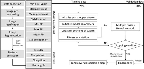
The performance of the optimization algorithm initially depended on the proper setting of its parameters. The first group identified the structure of the neural network by defining an optimal number of hidden neurons in the hidden layer. We found that, from literature, the optimal number should be less than the input nodes (52 predictor variables in this case) and larger than output nodes (4 land surface classes). By running several trials, we decided to select ten hidden neurons as the model generated highest RMSE with this setting. Thereofre, n-variable from (Figure 3) was replaced with 10. The typical topology for this experiment consisted of 52 inputs, ten hidden neurons, and four output classes. The second group of GOA was defined as follows: Maximum iteration was set to 500; low bound and upbound were −1 and 1; swarm population or number of grasshopper was 100; cMax = 1; cMin = 0.00004; fitness function was set as in (Equation 3). Those parameters were kept constant for other runs with different training sizes. Detail description of parameters of GOA in comparison with GWO and BBO is shown in Table 3

The initial swarm was generated, in which positions of grasshoppers were defined as 560-dimensions space (representing 560 weight parameters of the multiple-class neural network that equal to 52 predictor variables multiplied by ten hidden neurons +10 hidden neurons multiplied by four output classes). The best values for these weights were determined through optimization iteration of the training process. For each iteration, RMSE as in (Equation 3) was used as the fitness function. This hybrid model was iterated for 500 times.

4. Results and discussion

To examine the model consistency over the study area, we tested several scenarios with different data size. Based on segmented objects as described in the previous section, we selected a subset of 4000, 2000, and 400 objects. The objects were randomly selected across the diverse surface morphology of the study area, and each of the subsets included equal percentages of the four classes (water, vegetation, impervious surface, and bare soil). The general procedure for data preparation and model initialization for each run is described in section 3.

GMNN was initialized and ran for the first trial with 4000 objects. The model operated and stopped when the iteration process reached 500 with the smallest objective value. It could be observed that RMSE of GOA dramatically dropped at around the 190th iteration and gradually decreased from iteration 210. GOA overcame GWO and BBO around iteration 220 and from this point, all three curves ran almost horizontally until reaching iteration 500. It could be seen that GOA ended up with RMSE was 0.2225, which was smaller than RMSE from other methods as shown in (Table 4) (Figure 5).

Figure 5. Neural network optimized GOA after 500 iteration.

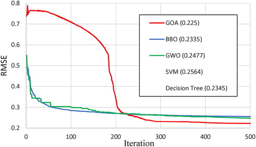
Table 4. Accuracy assessment for 4000 training objects (best values in shaded cells).

Classifier/Base classifier	Optimization algorithm	RMSE	MAE	Kappa	Overall Accuracy
MNN	GWO	0.2477	0.0902	0.7685	83.2381
MNN	BBO	0.2335	0.1129	0.7843	84.4762
MNN	GOA	0.2225	0.1086	0.8284	87.1905
DT		0.2345	0.1244	0.7848	84.4771
SVM		0.2564	0.1221	0.7503	82.0012

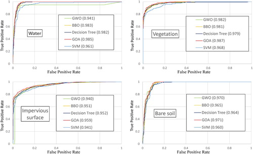
Optimal parameters from the 500th iteration were used in MNN to classify objects in the validation dataset. The accuracies for land cover classification are shown in (Table 4) with four performance indicators. By comparing the area under ROCs for each category (Figure 6), GMNN outperformed the remaining algorithms in all separate four land cover type extractions. Specifically, GMNN achieved AUC at 0.985 for water extraction, 0.987 for vegetation type, 0.959 for impervious surface and 0.971 for bare soil class. In addition, both RMSE and overall accuracy of GMNN were better than the remaining methods, which validated its ability in multiple class classification. MAE of GMNN was also smaller than the other three but slightly larger than MNN optimized by GWO (GWO-MNN). This is due to GWO-MNN generating a larger variance associated with the frequency distribution of error, which makes RMSE of GWO-MNN higher than GMNN.

Figure 6. ROCs and AUC values for 4000 training objects.

Overall accuracy measured the overall performance of models. However in some cases, the extraction of specific surface type is the most important for different applications (Duro, Franklin, and Dubé 2012; Huang et al. 2015). For multiple-class classification, the proposed model generated four percentage values that determine the probabilities for each segment to be placed in one of the four targeted classes. If each surface cover was to be separately investigated, the overall accuracy of the classification would be significantly improved.

In some cases, machine learning algorithms are found to be sensitive to sample sizes as they remain robust with larger training size but accuracies decrease with smaller training data (Duro, Franklin, and Dubé 2012; Im et al. 2012). GMNN and other algorithms were also examined by using two different subsets of 2000 and 400 objects. The results are shown in (Tables 5 and 6) and (Figures 7 and 8), which reaffirmed the classifiable capability of GMNN over the other algorithms. GMNN resulted in the smallest RMSE and the highest overall accuracy, kappa index. GMNN also outperformed the others in classifying single classes with higher AUC values, except AUC for bare soil. In these cases, BBO-MNN was slightly higher than GMNN (Figure 7) and DT was better than GMNN (Figure 8). For land cover classification, when the error costs of missclassification of all classes are unknown or equal, the ROC curves are useful for exploring the tradeoffs between classes. Therefore finding the optimal sizes for the training datasets for each type of land covers will be important, particularly for the detection of specific pattern.

Figure 7. ROCs and AUC values for 2000 training objects.

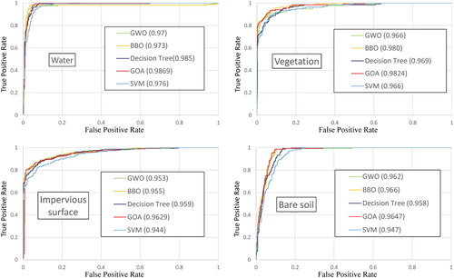
Figure 8. ROCs and AUC values for 400 training objects.

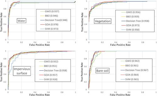
Table 5. Accuracy assessment for 2000 training objects (best values in shaded cells).

Classifier/Base classifier	Optimization algorithm	RMSE	MAE	Kappa	Overall Accuracy
MNN	GWO	0.2337	0.0846	0.798	0.853333
MNN	BBO	0.2241	0.112	0.799	0.854667
MNN	GOA	0.2217	0.0866	0.8136	0.869300
DT		0.2375	0.1309	0.7759	0.838667
SVM		0.258	0.1238	0.7348	0.809333

Table 6. Accuracy assessment for 400 training objects (best values in shaded cells).

Classifier/Base classifier	Optimization algorithm	RMSE	MAE	Kappa	Overall Accuracy
MNN	GWO	0.2826	0.1033	0.7242	0.802
MNN	BBO	0.2447	0.1043	0.777	0.840
MNN	GOA	0.2373	0.1029	0.7836	0.844
DT		0.2414	0.1299	0.7715	0.836
SVM		0.267	0.1316	0.7353	0.806

An additional test was carried out to determine whether the performance of models was statistically different. Non-parametric Wilcoxon signed-rank test was chosen as the dependent variable was measured in nominal scale. Each pair of two models was tested by using AUC values with Null hypothesis stating that there was no difference between the predictive capability of the two selected model. The results in (Table 7) show that all p values are smaller than 0.05 that the null hypothesis would be rejected and the differences were statistically significant. The differences in performance between classification methods could be caused by either the predictive capability of the techniques or the variation within the dataset. Nonetheless, in this study, several training datasets randomly selected across heterogenous urban morphology and then classified by our proposed model and benchmark classifiers show that, from all trials, GMNN significantly improved both the overall accuracy and detection accuracy of each land surface. Therefore, with its robustness, this method can be used in urban applications to partially satisfy the requirements of planners in detecting detailed change patterns in a metropolitan area.

Table 7. Wilcoxon signed-rank test.

Pairwise comparison	p-value (<0.05)	Significance
GMNN vs. GWO-MNN	0.0004883	Yes
GMNN vs. BBO-MNN	0.003216	Yes
GMNN vs SVM	0.0009766	Yes
GMNN vs. DT	0.007602	Yes

5. Map generation

To visually display the classification capabilities of GMNN, we produced three maps using the trained models with three different training and validation datasets. (Table 8) shows the sample output of the model, as each object was assigned four probability values of being assigned to one of the four classes. For the entire study area, more than 54.000 objects were classified based on probability values. The results are shown in (Figure 9). It could be seen that three maps were almost identical in water class. The misclassified objects were mainly between impervious and bare soil because of the mixture between two types. Although overall accuracies of three cases were quite similar, the spatial placement of misclassified objects resulted in more fragmented patterns in maps associated with smaller training datasets.

Figure 9. Subsets of classified maps by GMNN with different training and validation sizes. From left to right: 4000 objects, 2000 objects, 400 objects.

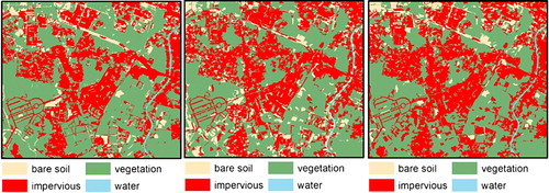
Table 8. Sample of probability assignments.

Predicted classes	Prob of being Vegetation	Prob of being Water	Prob of being Bare soil	Prob of being Impervious
water	0	0.973	0.026	0
bare soil	0.222	0.098	0.655	0.024
vegetation	0.955	0	0	0.045
vegetation	0.967	0	0	0.033
vegetation	0.986	0.001	0	0.013
impervious	0.002	0.095	0	0.903
water	0.036	0.832	0.014	0.118
water	0	0.672	0.328	0

6. Conclusion and future remarks

Machine learning has been widely used in remote sensing as mining techniques to support classifying land surface patterns in either high spatial resolution or multiple spectral resolutions. This study verified this trend by successfully integrating GOA into MNN for urban pattern detection in Hanoi. This novel method was robust in classifying all four types of urban surface as it outperformed other established classifiers with regards to overall accuracies and separate AUCs. The overall accuracy of around 87% for a spatially varied study area is the affirmative reasoning for its applicability in other urban regions. Though this value was measured by multiplying extraction accuracies of four classes, the extraction accuracy of any single class was much higher, and that would be very useful for specific applications of certain types of urban land cover.

The consistency of classification algorithms is normally subject to variation of training sample sizes. However, it was not the case in this study as GMNN seemed to be robust in all three training and validation datasets. The success of this model was dependent on the proper selection of model parameters as they were determined through trial-error processes, and these values were found suitable for the dataset of the study area. Therefore, settings might need to be changed when this method is used with another study area with diverse surface morphology. The performance of this hybrid model indicates a vast potential for the implementation of meta-heuristic algorithms in object-based classification. In this case, GOA was more powerful than GWO and BBO, but it might be different if another dataset was used.

Finally, this model was applied for high spatial resolution data but might be applicable for a variety of mid-resolution satellite data such as Landsat or Sentinel. Therefore, more effort should be spent on examining those kinds data and automating the image processing workflow to derive land cover types, particularly in larger urban areas.

Disclosure statement

No potential conflict of interest was reported by the authors.

ORCID

Quang-Thanh Bui http://orcid.org/0000-0002-5059-9731

Additional information

Funding

This research is funded by Vietnam National Foundation for Science and Technology Development (NAFOSTED) under Grant Number [105.99-2016.05].

References

- Abhishek G Neve, G. M. K. a. O. K. 2017. “Application of Grasshopper Optimization Algorithm for Constrained and Unconstrained Test Functions.” International Journal of Swarm Intelligence and Evolutionary Computation 6 (3). doi:10.4172/2090-4908.1000165.
- Belgiu, M., and L. Drăguţ. 2016. “Random Forest in Remote Sensing: A Review of Applications and Future Directions.” ISPRS Journal of Photogrammetry and Remote Sensing 114 (Supplement C): 24–31. https://doi.org/10.1016/j.isprsjprs.2016.01.011.
- Chan, J. C.-W., and D. Paelinckx. 2008. “Evaluation of Random Forest and Adaboost Tree-Based Ensemble Classification and Spectral Band Selection for Ecotope Mapping Using Airborne Hyperspectral Imagery.” Remote Sensing of Environment 112 (6): 2999–3011. https://doi.org/10.1016/j.rse.2008.02.011.
- Dou, J., K.-T. Chang, S. Chen, P. A. Yunus, J.-K. Liu, H. Xia, and Z. Zhu. 2015. “Automatic Case-Based Reasoning Approach for Landslide Detection: Integration of Object-Oriented Image Analysis and a Genetic Algorithm.” Remote Sensing 7 (4). doi:10.3390/rs70404318.
- Duro, D. C., S. E. Franklin, and M. G. Dubé. 2012. “A Comparison of Pixel-Based and Object-Based Image Analysis with Selected Machine Learning Algorithms for the Classification of Agricultural Landscapes Using SPOT-5 HRG Imagery.” Remote Sensing of Environment 118 (Supplement C): 259–272. https://doi.org/10.1016/j.rse.2011.11.020.
- Gong, B., J. Im, and G. Mountrakis. 2011. “An Artificial Immune Network Approach to Multi-Sensor Land use/Land Cover Classification.” Remote Sensing of Environment 115 (2): 600–614. https://doi.org/10.1016/j.rse.2010.10.005.
- Hamedianfar, A., H. Z. M. Shafri, S. Mansor, and N. Ahmad. 2014. “Combining Data Mining Algorithm and Object-Based Image Analysis for Detailed Urban Mapping of Hyperspectral Images.” Journal of Applied Remote Sensing 8 (1): 085091. doi:10.1117/1.JRS.8.085091.
- Herold, S., and M. C. Sawada. 2012. “A Review of Geospatial Information Technology for Natural Disaster Management in Developing Countries.” International Journal of Applied Geospatial Research 3 (2): 24–62. doi:10.4018/jagr.2012040103.
- Huang, X., C. Xie, X. Fang, and L. Zhang. 2015. “Combining Pixel- and Object-Based Machine Learning for Identification of Water-Body Types From Urban High-Resolution Remote-Sensing Imagery.” IEEE Journal of Selected Topics in Applied Earth Observations and Remote Sensing 8 (5): 2097–2110. doi:10.1109/JSTARS.2015.2420713.
- Im, J., Z. Lu, J. Rhee, and L. J. Quackenbush. 2012. “Impervious Surface Quantification Using a Synthesis of Artificial Immune Networks and Decision/Regression Trees From Multi-Sensor Data.” Remote Sensing of Environment 117 (Supplement C): 102–113. https://doi.org/10.1016/j.rse.2011.06.024.
- Jonkman, S., and R. Dawson. 2012. “Issues and Challenges in Flood Risk Management – Editorial for the Special Issue on Flood Risk Management.” Water 4 (4): 785–792.
- Lary, D. J., A. H. Alavi, A. H. Gandomi, and A. L. Walker. 2016. “Machine Learning in Geosciences and Remote Sensing.” Geoscience Frontiers 7 (1): 3–10. https://doi.org/10.1016/j.gsf.2015.07.003.
- Mirjalili, S., S. M. Mirjalili, and A. Lewis. 2014. “Grey Wolf Optimizer.” Advances in Engineering Software 69: 46–61. http://doi.org/10.1016/j.advengsoft.2013.12.007.
- Mountrakis, G., J. Im, and C. Ogole. 2011. “Support Vector Machines in Remote Sensing: A Review.” ISPRS Journal of Photogrammetry and Remote Sensing 66 (3): 247–259. https://doi.org/10.1016/j.isprsjprs.2010.11.001.
- Myint, S. W., P. Gober, A. Brazel, S. Grossman-Clarke, and Q. Weng. 2011. “Per-pixel vs. Object-Based Classification of Urban Land Cover Extraction Using High Spatial Resolution Imagery.” Remote Sensing of Environment 115 (5): 1145–1161. https://doi.org/10.1016/j.rse.2010.12.017.
- Nguyen, T. H. T., V. T. Tran, Q. T. Bui, Q. H. Man, and T. d. V. Walter. 2016. “Socio-economic Effects of Agricultural Land Conversion for Urban Development: Case Study of Hanoi, Vietnam.” Land Use Policy 54: 583–592. http://doi.org/10.1016/j.landusepol.2016.02.032.
- Petropoulos, G. P., C. Kalaitzidis, and K. Prasad Vadrevu. 2012. “Support Vector Machines and Object-Based Classification for Obtaining Land-use/Cover Cartography From Hyperion Hyperspectral Imagery.” Computers & Geosciences 41 (Supplement C): 99–107. https://doi.org/10.1016/j.cageo.2011.08.019.
- Qian, Y., W. Zhou, J. Yan, W. Li, and L. Han. 2015. “Comparing Machine Learning Classifiers for Object-Based Land Cover Classification Using Very High Resolution Imagery.” Remote Sensing 7 (1). doi:10.3390/rs70100153.
- Saremi, M., S. Mirjalili, and A. Lewis. 2017. “Grasshopper Optimisation Algorithm: Theory and Application.” Advances in Engineering Software 105 (Supplement C): 30–47. https://doi.org/10.1016/j.advengsoft.2017.01.004.
- Simon, D. 2008. “Biogeography-Based Optimization.” IEEE Transactions on Evolutionary Computation 12 (6): 702–713. doi:10.1109/TEVC.2008.919004.
- Wieland, M., and M. Pittore. 2014. “Performance Evaluation of Machine Learning Algorithms for Urban Pattern Recognition From Multi-Spectral Satellite Images.” Remote Sensing 6 (4): 2912–2939. doi:10.3390/rs6042912.
- Yuri, Z. (2002, 24-28 June 2002). A new Automatic Approach for Effectively Fusing Landsat 7 as Well as IKONOS Images. Paper presented at the IEEE international geoscience and remote sensing symposium.
- Zhou, W., and A. Troy. 2008. “An Object-Oriented Approach for Analysing and Characterizing Urban Landscape at the Parcel Level.” International Journal of Remote Sensing 29 (11): 3119–3135. doi:10.1080/01431160701469065.
- Zhou, W., and A. Troy. 2009. “Development of an Object-Based Framework for Classifying and Inventorying Human-Dominated Forest Ecosystems.” International Journal of Remote Sensing 30 (23): 6343–6360. doi:10.1080/01431160902849503.