Snow depth and ice thickness derived from SIMBA ice mass balance buoy data using an automated algorithm

ABSTRACT

An ice mass balance buoy (IMB) monitors the evolution of snow and ice cover on seas, ice caps and lakes through the measurement of various variables. The crucial measurement of snow and ice thickness has been achieved using acoustic sounders in early devices but a more recently developed IMB called the Snow and Ice Mass Balance Array (SIMBA) measures vertical temperature profiles through the air-snow-ice-water column using a thermistor string. The determination of snow depth and ice thickness from SIMBA temperature profiles is presently a manual process. We present an automated algorithm to perform this task. The algorithm is based on heat flux continuation, limit ratio between thermal heat conductivity of snow and ice, and minimum resolution (±0.0625°C) of the temperature sensors. The algorithm results are compared with manual analyses, in situ borehole measurements and numerical model simulation. The bias and root mean square error between algorithm and other methods ranged from 1 to 9 cm for ice thickness counting 2%–7% of the mean observed values. The algorithm works well in cold condition but becomes less reliable in warmer conditions where the vertical temperature gradient is reduced.

KEYWORDS:

• Snow
• sea ice
• ice thickness
• ice mass balance buoy
• polar oceans

1. Introduction

Sea ice covers some 6%–7% of the Earth's surface, mostly in the Arctic and Antarctic (Thomas and Dieckmann 2008). Basic information on the sea ice pack, such as sea ice extent (SIE), sea ice concentration (SIC), and sea ice thickness (SIT), can be retrieved using space-borne observations (Laxon et al. 2013). Passive microwave satellite data reveal that since 1979, late summer and early autumn sea ice extent has decreased by approximately 40%, and a combination of historical submarine observations and recent satellite data show that winter sea ice thickness has simultaneously decreased by 50% (Kwok and Cunningham 2015). Climate-warming in the Arctic has been twice the rate of the global average (Overland et al. 2016). The most dramatic indicators of Arctic warming have been the decrease in the SIE, SIC, and SIT, as well as the duration of the ice season (Döscher, Vihma, and Maksimovich 2014). The minimum sea ice extent on 10 September 2016 ranked the second lowest value in history. It was equivalent to a mere 50% of the average value from 1981–2010. The strong decline in sea ice cover is expected to continue, with estimates for a practically ice-free Arctic in late summer around the year 2050 (Overland, Wood, and Wang 2011).

Sea ice is a critical component of the climate system in the polar oceans and plays an important role in the global climate system; therefore, accurate monitoring of sea ice cover is critical (Vihma 2014). The ocean-atmosphere exchanges of heat, momentum, and gases are strongly affected by sea ice thickness distribution. The growth of sea ice is strongly dependent on the heat exchange at the ice/water interface, on radiation and turbulent heat fluxes at the ice/snow surface, and on snow depth. A thin layer of sea ice allows a large conductive heat flux upward through the ice, resulting in a high ice surface temperature, which further affects air temperature.

There are a large number of methods used to measure snow depth and ice thickness, such as a satellite altimeter to measure ice elevations (freeboard), aircraft electromagnetic induction (EM) sounding, submarine upward looking sonar (ULS), sea floor mooring, ice mass balance (IMB) drift buoys, and thickness gauges. The thickness gauges provide the most accurate snow depth and ice thickness measurements and are often used for ground truth. However, thickness gauges require manual operation and can only be obtained during limited field campaigns. In addition, the measurements obtained often have coarse spatial and temporal resolutions. Therefore, autonomous ice mass balance (IMB) drift buoys are more effective and can obtain seasonal variations in snow depth and ice thickness with better spatial and temporal coverages (Perovich et al. 2003).

The first classical IMB buoys were developed by the U.S. Cold Regions Research and Engineering Laboratory (CRREL) jointly with MetOcean Ltd., Canada. This type of buoy is usually deployed on thick multi-year ice floes to ensure a long lifespan. The CRREL IMB is equipped with acoustic sounders mounted in the air and below the ice base. Distances between the downward-looking sounder and the snow surface and the upward-looking sounder and the ice bottom are measured. The initial snow/ice interface is defined as the reference level, so the measured distances easily convert to snow depth, surface ice ablation, and ice bottom growth and ablation. Eventually, snow depth and ice thickness can be obtained (Rösel et al. 2016). A thermistor string is vertically deployed through the air, snow, and ice into the upper ocean to measure the temperature field within these materials. CREEL IMB also measures the GPS position, sea level pressure, and surface air temperature. The IMBs are anchored on an ice floe at fixed locations, and the buoy takes automatic measurements along the ice drift trajectory at predefined intervals. The data are transmitted via Iridium satellite. This type IMB has been widely used in the Arctic Ocean. For example, Perovich and Richter-Menge (2015) accessed the data of 41 IMBs covering deployment from 1957 to 2014 to investigate the regional variability in the sea ice mass balance.

Another type of IMB has been developed by the Scottish Association for Marine Science (SAMS) Research Services Ltd (SRSL) based at the Scottish Marine Institute, UK. This type of IMB is referred to as a high-resolution snow and ice mass balance array (SIMBA) and is equipped with a 5-m-long thermistor string with sensors spaced every 2 cm (Jackson et al. 2013). SIMBA buoys have built-in GPS to record buoy drift positions, a magnetometer for tilt and floe rotation, a barometer for surface air pressure, and one external sensor to measure near-surface ambient air temperature. In addition, a resistor component is mounted immediately underneath every thermistor sensor. A weak voltage (8 V) supply is connected to create gentle heating of each sensor and its surroundings. The heating interval usually lasts for one (60 s) or two minutes (120 s). The rise of temperature in the 120 s is approximately 2°C in the air and 0.2°C in the ice and water (Jackson et al. 2013). Sensor heating occurs once per day. The temperature change is used to identify air/snow, air/ice, and ice/water interfaces. The Iridium satellite is used for data transmission. Compared with the CRREL IMB, the SIMBA buoy is low cost, making it possible to be deployed in large numbers across the Arctic Ocean. This reduces the risk of failure of an observation campaign. SIMBA data has been used for snow depth and ice thickness monitoring and energy balance studies in seasonally ice-covered lakes, seas, and for polar ice cover (Cheng et al. 2014; Hoppmann et al. 2015; Provost et al. 2017; Lei et al. 2018). However, the retrieval of snow depth and ice thickness from SIMBA temperature profiles is not a trivial task. Sensors exposed in the air could be affected by the high-frequency variations in the near-surface boundary layer, such as wind vibration, snow drift, frost condensation, and solar heating. These changes could result in erroneous temperature readings. Without acoustic sounders, any erroneous temperature readings will make it impossible to obtain snow depth and ice thickness from SIMBA. So far, SIMBA data analyses are primarily a manual process. A unified data processing technique to reliably and accurately determine sea ice thickness and snow depth from this kind of data is still missing, and an unambiguous interpretation remains a challenge.

In this study, a mathematically and physically based algorithm is developed to process SIMBA temperature data to retrieve snow depth and ice thickness systematically and automatically. The algorithm is tested in terms of two SIMBA deployment scenarios: (1) bare ice and (2) ice covered with snow. The algorithm is then coded with two modules targeting archived historical or online near real-time SIMBA data. The results are compared with manual analyses and in situ observations. This is the initial step toward the establishment of a monitoring system for snow depth and ice thickness in the Arctic Ocean that can provide sustainable repeatability.

2. Algorithm principle

The algorithm required the following assumptions: (1) thermodynamic changes in snow and ice temperature are faster than thermodynamic changes in snow depth and ice thickness; (2) in cold conditions, the temperature profiles of snow and ice are piecewise linear because of the large difference between snow and ice thermal conductivities (Leppäranta,1983); (3) in idealized conditions, the vertical temperature gradient in a short distance (<1  m) in the air above the surface is assumed to be negligible; and (4) the temperature difference in water below the ice bottom is assumed to be a constant freezing temperature.

The SIMBA digital thermistor sensor is the Maxim DS28EA00 with 12-bit (1/16°C) resolution (Jackson et al. 2013). This means the minimum temperature change that can be detected by the thermistor sensor is 0.0625°C. Therefore, assuming there are two sensors placed with a distance of Δx between them, the measured temperature difference between these two sensors cannot be smaller than |ΔT| = 0.0625°C.

Two scenarios of SIMBA deployment were considered (Figure 1). The vertical heat conduction and temperature distribution satisfy the continuity (Parkinson and Washington 1979), as shown in the following equation:(1) $k_s\frac{\mathrm{\partial }{T}_s}{\mathrm{\partial }{z}_s}=k_i\frac{\mathrm{\partial }{T}_i}{\mathrm{\partial }{z}_i},$(1) where T is the temperature; k represents the thermal heat conductivity of the material, which is a measure of the ability of a material to conduct heat; and z is the vertical positive downward coordinate. The subscripts, s and i, represent snow and ice, respectively. Under standard atmospheric pressure and zero temperature, the thermal heat conductivities of air (0.024 W/mK), snow (∼0.2 W/mK), ice (∼2.1 W/mK), and water (0.58 W/mK) are considerably different from each other. The corresponding specific heat capacities of air, snow/ice, and water are 1004 J/kgK, 2093 J/kgK, 4180 J/kgK, respectively (Yen 1981). In a steady state, the temperature gradient due to heat transfer through these materials is different. In snow, for example, the vertical temperature gradient is much larger compared to that in ice, because snow has a low thermal heat conductivity and acts as an insulator on top of the ice.

Figure 1. The vertical structure of SIMBA deployment scenarios (a): air–ice–water and (b) air–snow–ice–water. k_i and k_s are the thermal heat conductivity of ice and snow for each layer (numbers in parentheses) between two thermistor sensors (horizontal lines). The dotted lines are sensor locations in the air and water. The interval between two sensors is 2 cm.

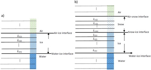
The heat conductivities of snow and ice are likely to change along the vertical direction because of impurities and different crystal structures (Sturm et al. 1997; Pringle et al. 2007). However, within a certain depth, such as 2 cm, k_s and k_i can be treated as constants (Pringle et al. 2007). The SIMBA thermistor sensors have a 2-cm constant interval along the thermistor string. Applying the continuity assumption, the thermal heat conduction between two adjoined layers (x and x + 1) in snow and (y and y + 1) layers in ice are:(2) $k_{s\left(x\right)}\frac{\mathrm{\partial }{T}_{s\left(x\right)}}{\mathrm{\partial }{z}_{s\left(x\right)}}=k_{s\left(x+1\right)}\frac{\mathrm{\partial }{T}_{s\left(x+1\right)}}{\mathrm{\partial }{z}_{s\left(x+1\right)}},x=1,2,3,\dots ,m-1,$(2) (3) $k_{i\left(y\right)}\frac{\mathrm{\partial }{T}_{i\left(y\right)}}{\mathrm{\partial }{z}_{i\left(y\right)}}=k_{i\left(y+1\right)}\frac{\mathrm{\partial }{T}_{i\left(y+1\right)}}{\mathrm{\partial }{z}_{i\left(y+1\right)}},y=1,2,3,\dots ,n-1,$(3) where x and y represent the number of layers in snow and ice, respectively. At the snow/ice interface, the following holds true:(4) $k_{s\left(m\right)}\frac{\mathrm{\partial }{T}_{s\left(m\right)}}{\mathrm{\partial }{z}_{s\left(m\right)}}=k_{i\left(1\right)}\frac{\mathrm{\partial }{T}_{i\left(1\right)}}{\mathrm{\partial }{z}_{i\left(1\right)}},$(4) where the total number of layers in snow and ice are m and n, respectively (Figure 1), and snow and ice heat conductivity in each layer are labeled as k_s(x), k_i(y), respectively. Because the space between two sensors is constant, we can rewrite Eqs. (2)–(4) to form the finite differences:(5a) $\mathrm{\Delta }{T}_{s\left(x\right)}=\frac{k_{s\left(x+1\right)}}{k_{s\left(x\right)}}\mathrm{\Delta }{T}_{s\left(x+1\right)},\left(1\le x\le m-1\right),\left(5\mathrm{a}\right)$(5a) (5b) $\mathrm{\Delta }{T}_{i\left(y\right)}=\frac{k_{i\left(y+1\right)}}{k_{i\left(y\right)}}\mathrm{\Delta }{T}_{i\left(y+1\right)},\left(1\le y\le n-1\right)\left(5\mathrm{b}\right)$(5b) where Δ represents the temperature difference between the two sensors. For example, ΔT_s(x) =T_s(x+1)–T_s(x), ΔT_s(x+1) =T_s(x+2)–T_s(x+1), ΔT_i(y) =T_i(y+1)–T_i(y), and ΔT_i(y+1) =T_i(y+2)–T_i(y+1). Based on the fact of heat flux continuation, for the first deployment scenario (the only ice condition):(6a) $\mathrm{\Delta }{T}_{i\left(y\right)}=\frac{k_{i\left(n\right)}}{k_{i\left(y\right)}}\mathrm{\Delta }{T}_{i\left(n\right)},\left(1\le y\le n\right),\left(6\mathrm{a}\right)$(6a) and for the second deployment scenario (ice with snow on top condition):(6b) $\mathrm{\Delta }{T}_{s\left(x\right)}=\frac{k_{i\left(y\right)}}{k_{s\left(x\right)}}\mathrm{\Delta }{T}_{i\left(y\right)}=\cdots =\frac{k_{i\left(n\right)}}{k_{s\left(x\right)}}\mathrm{\Delta }{T}_{i\left(n\right)},\left(1\le x\le m,1\le y\le n\right).\left(6\mathrm{b}\right)$(6b)

The thermal conductivity of seasonal snow is largely dependent on the density (Sturm et al. 1997). It varies from 0.1 W/mK for very fresh snow up to 0.6 W/mK for very hard wind compacted snow (Yen 1981). In the Arctic, we can assume k_s ranges from 0.1 to 0.3 W/mK between two adjoined layers (Merkouriadi et al. 2017). The in situ measurement of sea ice thermal heat conductivity is from 1.88 ± 0.13 W/mK for multiyear sea ice to 2.13 ± 0.13 W/mK for first year sea ice (Pringle et al. 2007). Therefore,(7a) $\frac{k_{i\left(n\right)}}{k_{i\left(y\right)}}\in \left[\frac{1.9}{2.3},\frac{2.3}{1.9}\right]\sim \left[0.831.21\right]\left(1\le y\le n\right)\left(7\mathrm{a}\right)$(7a) (7a′) $\frac{k_{i\left(n\right)}}{k_{i\left(y\right)}}\le 2\left(1\le y\le n\right),\left(7{\mathrm{a}}^{\mathrm{\prime }}\right)$(7a′) (7b) $\frac{k_{i\left(n\right)}}{k_{s\left(x\right)}}\in \left[\frac{1.9}{0.3},\frac{2.3}{0.1}\right]\sim \left[6.323\right]\left(1\le x\le m\right),\left(7\mathrm{b}\right)$(7b) (7b′) $\frac{k_{i\left(n\right)}}{k_{s\left(x\right)}}\ge 7\left(1\le x\le m\right),\left(7{\mathrm{b}}^{\mathrm{\prime }}\right)$(7b′) (7c) $\mathrm{\Delta }{T}_{i\left(n\right)}\in \left[0.5\times 0.0625,1.5\times 0.0625\right].\left(7\mathrm{c}\right)$(7c)

The minimum temperature resolution of thermistor sensors is 0.0625°C. This means if the temperature change of one sensor or between two adjoined sensors is less than 0.5 × 0.0625°C, the recorded temperature change will be zero, i.e. the sensor readings will remain the same. Conversely, if the temperature change reaches between 0.5 × 0.0625°C and 1.5 × 0.0625°C, the recorded temperature change will be 0.0625°C. Therefore, according to (6a), (7a), and (7a′),(8a) $0.0625<\mathrm{\Delta }{T}_{i\left(y\right)}\le 2\ast \mathrm{\Delta }{T}_{i\left(n\right)}\left(1\le y\le n\right),\left(8\mathrm{a}\right)$(8a) or(8b) $0.0625\le \left|\mathrm{\Delta }{T}_{ice}\right|\le \mathrm{0.1875.}\left(8\mathrm{b}\right)$(8b)

Based on the same principle and according to (6b), (7b), and (7a′),(9a) $\mathrm{\Delta }{T}_{s\left(x\right)}>7\ast \left[0.0625\right]\left(1\le x\le m\right),\left(9\mathrm{a}\right)$(9a) or(9b) $\left|\mathrm{\Delta }{T}_{snow}\right|\ge \mathrm{0.4375.}\left(9\mathrm{b}\right)$(9b)

Finally,(10) $\left|\mathrm{\Delta }{T}_{snow}\right|\ge 0.4375>0.1875\ge \left|\mathrm{\Delta }{T}_{ice}\right|\ge \mathrm{0.0625.}$(10)

Equation (10) indicates that for any two adjoined sensors in the ice, the temperature difference should be less than or equal to 0.1875°C, while for two adjoined sensors in snow, the temperature difference should be larger than or equal to 0.4375°C. Data was searched for sensor temperature differences of 0.1875°C to identify air/ice interfaces and 0.4375°C to identify air/snow interfaces.

The vertical temperature gradient in air above the surface and in water below the ice bottom is very small. In snow and ice, a linear temperature profile was assumed for cold conditions. At each time step, the algorithm scans sensors from top to bottom multiple times to find a temperature criterion. Once the sensor temperature criteria match, a segment of thermistor string below this sensor will be searched to see if there is a consistent linear temperature gradient. If there is no temperature criteria found, then the interface position will be defined based on the value in the previous step.

The ice bottom position is detected based on a statistical calculation. A thermistor string section (e.g. 30 sensors) is defined that is partly in the ice and partly in the water. This is possible since there are always sensors placed in the water, and the initial deployment status or the ice bottom position at the previous time step is known. The temperature of seawater close to the ice bottom is stable near the freezing point. As a result, the minimum temperature difference between two adjoined sensors ranges between 0.5 and 1.5 × 0.0625°C theoretically. The temperature reading of these 30 sensors is collected as a time series. The temperature value that appears most in the time series is then specified as the freezing temperature, T_f (t) at time step (t). The temperatures of these 30 sensors are then read from bottom up, and the last sensor position that has the T_f (t) value is identified as the ice bottom at step (t).

Data quality control is carried out to remove unrealistic and erroneous temperature profiles. SIMBA temperature measurements are collected four times a day. To minimize the impact of solar heating, temperature profiles measured during the night are also collected.

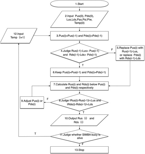
The algorithm is implemented in Matlab. The number input parameters are (1) the initial sensor positions at interfaces; (2) the daily assumed maximum snow depth and ice thickness evolution, and (3) the maximum measureable snow depth and ice thickness. Initial sensor positions are recorded during deployment. The maximum snow depth and ice thickness allowed in one day are empirical parameters and largely based on in situ observations and simple climatological analyses. In the Arctic Ocean, a snowfall event can create a daily snow accumulation of approximately 20 cm during the summer (Zhang 2004). During the winter, however, the daily snow accumulation can be much smaller because of strong winds. A recent field measurement has indicated that a single extensive snowstorm can create 6 cm of snow accumulation in one day (Sturm et al. 1997). Accordingly, the threshold SIMBA daily snow depth change is assumed to be no more than 15 sensors distances (30 cm). Daily ice thickness growth or ablation largely depends on weather conditions and the initial thickness of the ice. Assuming the initial ice thickness is 0.05  m and 1.0  m, the classical Stefan law yields 6 cm and 0.3 cm daily ice growth, respectively, during cold weather conditions, with a daily mean air temperature of -10°C. Hence, the maximum daily ice thickness change rate is assumed to be a five sensor distance (10 cm). The maximum SIMBA snow depth and ice thickness are naturally limited by the total integrated sensor distance when they are initially placed in the air and water, respectively. The algorithm operation flow chart is given in Figure 2. The SIMBA thermistor sensors are numbered from top (1) in the air down to (240) in the water. The name list of several parameters are the following:

Figure 2. Flow diagram of the algorithm (RT module, see Section 3.3 for details).

Pas: Initial position of snow or ice surface.

Psi: Initial position of snow/ice interface.

Piw: Initial position of ice bottom.

Lus: Threshold of surface change (snowfall or ablation) in one day (e.g. 30 cm/day).

Lds: Threshold of ice bottom change (growth or ablation) in one day (e.g. 10 cm /day).

Pus(i): First guess of top surface sensor position for day (i); Pus (0): initial top surface sensor position for snow or ice surface == Pas.

Pds(i): First guess of ice bottom sensor position for day (i); Pds (0) initial ice bottom sensor position == Piw;

Temp(i): SIMBA temperature profile for the day (i). Temp (0): SIMBA temperature profile, first input.

Rus(i): Result of top surface for day (i). Rus (0) = Pas.

Rds(i): Result of ice bottom for day (i). Rds (0) = Piw.

Pus(0): Start from 1/3 total number of sensors in the air. For example, if there are 50 sensors placed vertically in the air from top to the surface, then Pus(0) = 16 The Pds(0) = Piw – 5 sensors. Lus and Lds are used to correctly identify the snow or ice surface and ice bottom, respectively. The algorithm assumes Psi remain unchanged during the SIMBA working period. The ice bottom is at freezing temperature. The algorithm scans sensor numbers from top (1) down to the end of the thermistor string (240) in water to identify snow or ice surface and the ice bottom. The final snow depth and ice thickness are calculated based on the identified interface sensor positions.

3. Results and discussion

The algorithm was tested to retrieve snow depth and ice thickness from approximately ten SIMBA buoys. In this study, the results from three selected cases are summarized (Table 1). The reason these three particular cases were selected are (1) the data from these SIMBA buoys had been investigated manually and the results could be used to compare with the algorithm output and (2) one SIMBA was deployed on sea ice without snow and in situ ice thickness was measured. Therefore, the algorithm could be validated for the bare ice scenario.

Table 1. SIMBA deployed in the Arctic and Antarctic ice-covered regions.

SIMBA IMEI	Deployment date	Initial snow depth (m)	Initial ice thickness (m)	Initial freeboard (m)	Termination date	Operational period (days)
A 300234010410200	22 Sep 2012	0.03	1.44	0.21	3 Aug 2013	315
B 300234060666760	29 Jan 2015	0.41	1.08	0.02	28 Feb 2015	30
C 300234061262820	11 May 2014	0.01	0.6	0.06	29 Nov 2014	223

3.1. Snow depth and ice thickness from SIMBA buoys

Buoy A was deployed in the high Arctic (88.8 N and 57.5 E) during the Polarstern Arctic cruise (ARK-XXVII/3) by the Alfred Wegener Institute (AWI) in 2012. Buoy B was deployed during the Norwegian young sea ICE (N-ICE2015) expedition in January 2015 (Granskog et al. 2016). These buoys were deployed on drift ice floes.

Buoy C was deployed on landfast sea ice in the vicinity of Zhongshan station in Prydz Bay, East Antarctic by the Chinese National Antarctic Research Expedition Program. The deployment was close to the shore, so the iridium data transmission was not activated, and buoy data were stored in an SD memory card. The in situ snow depths and ice thicknesses were measured on a weekly base. Boreholes were drilled through the ice, and the distance from the ice surface to the ice bottom was measured using an ice gauge. Snow thicknesses were measured with a stainless ruler from three close (<1  m) random sites near the ice boreholes (<2  m). The accuracy of ice and snow measurements was 0.01 and 0.005  m, respectively.

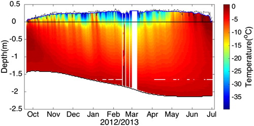
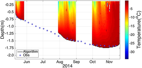
The observed snow and ice temperatures, as well as algorithm-derived snow depths and ice thicknesses from buoy A are shown in Figure 3. By the end of May, the snow depth was 32 cm and the ice thickness reached it seasonal maximum value of approximately 2.12  m. The climatological snow depth in the same region was approximately 33 cm in May (Warren et al. 1999). A few studies suggested that the ice thickness measured at that time and in that region was approximately 2.2  m. The snow depth increased by 30 cm and ice thickness by 68 cm. The snow depth showed occasional large diurnal variations. Without accurate in situ snow depth measurements, it is difficult to clarify whether those large temporal variations are real ground truth or artificially biased depths. To reduce uncertainty, a 5-day running mean surface elevation was calculated to represent seasonal snow depths.

Figure 3. SIMBA buoy A observed snow and ice temperature fields and algorithm retrieved snow depths and ice thicknesses. The blackline at zero level is the snow/ice interface. At the top, the dotted line is daily snow depth, and the solid line is the 5-day running mean snow depth.

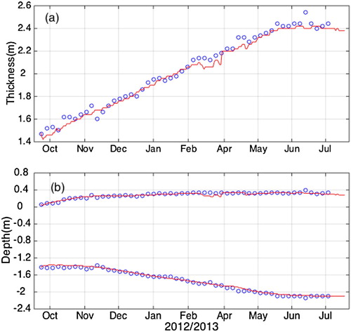
Buoy A data were investigated using manual analyses. The manual analyses are discussed in Zhao et al. (2017). The manual analyses selected one temperature profile every five days to identify snow depths and ice thicknesses because the thermodynamic mass balance of snow and sea ice does not change drastically in time. Figure 4 shows the results that were obtained using the algorithm and manual analyses. The total integrated snow and ice thicknesses yielded by both methods were similar to each other (Figure 4(a)).

Figure 4. (a) The total (snow + ice) thicknesses of buoy A obtained using the algorithm (solid line) and manual analyses (dots). (b) The snow depths and ice thicknesses derived using the algorithm (solid line) and manual analyses (dots). It was assumed that the snow/ice interface remained unchanged during the whole period.

Buoy B was deployed north of Svalbard on a first-year ice (FYI) floe, and it was operational from 29 January to 28 February 2015. Buoy B was part of the FMI contributions to the N-ICE2015 (Provost et al. 2017). The snow depths and ice thicknesses calculated using the algorithm are given in Figure 5. The lifetime of B was quite short. In February, there were several snowstorms (Itkin et al. 2017), where increasing snow depths and temperatures are clearly seen in the figure. The ice thickness shows a weak decreasing trend in February. The snow depths and ice thicknesses obtained using the algorithm are comparable to the results of Provost et al. (2017).

Figure 5. Snow depths and ice thicknesses of buoy B. The results from Provost et al. (2017) are shown as dashed lines.

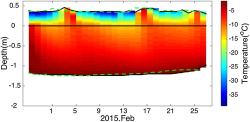
The operation of Buoy C lasted from May to November 2014. There was barely any snow onsite during the ice season because of a very strong eastern prevailing wind. Buoy C suffered a data storage problem. Therefore, temperature measurements were available only for three periods: May 11–28, July 31–September 1, and October 1–December 2. The algorithm was applied to these three periods. The results from the algorithm and in situ measurements are compared in Figure 6.

Figure 6. The Antarctic land-fast ice thicknesses. Observations (circles) versus algorithm-derived ice thicknesses (solid line).

3.2. Heating temperature regimen

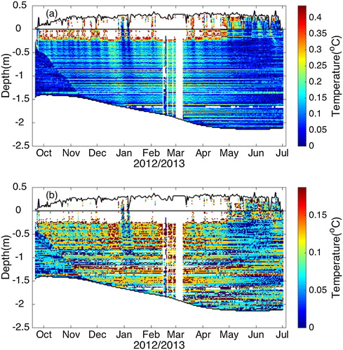
Each sensor on the SIMBA thermistor chain has a heating element. A small (8 V) voltage was applied to the resistors so that the heat energy liberated in the vicinity of each sensor would be the same. The heating time interval typically lasted from 60 to 120 s. The sensor temperatures usually rise by varying amounts along the thermistor chain based on whether their locations are in air, snow, ice, or water. In practice, however, the temperature changes may not be clear enough to detect the air/snow, snow/ice, and ice/water interfaces (Jackson et al. 2013). Consider buoy A as an example, the sensor temperature reading after 120 s of heating is plotted in Figure 6. Visual inspection reveals very weak discrimination of air/snow and ice/water interfaces from the colour pattern (Figure 7(a)). In June, the heating temperature showed no changes, but errors were probably encountered. The strong warm-up of the in-ice (∼1  m depth) in late December and mid-February (1  m –1.5  m depth) remain unknown.

Figure 7. (a) Heating temperatures regimen from 150 sensors placed vertically in the air–snow–ice–ocean column. The heating time interval was 120 s. The black circle marks the freezing pattern of the thermistor string borehole. The arrows point to the weak discrimination of interfaces. The white areas in December, February, and March are data missing periods. (b) Same plot as (a), but superimposed with air/snow and ice/ocean interfaces derived using the algorithm.

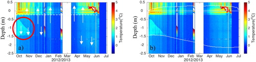
The heating temperature also revealed two horizontal discriminated interfaces at 0  m and –0.22  m in depth below the surface. The 0  m level was the original snow/ice interface. The second interface (white broken line in Figure 6(a)) is the original sea water level. The initial ice was thick (1.44  m), creating strong buoyancy that kept the upper part of the ice column above the water level. When SIMBA was deployed, the freeboard was 21 cm positive (sea water level was below ice surface), and this agreed well with the white broken line in Figure 7(a). When the SIMBA thermistor string was deployed, the positive freeboard introduced a segment of empty boreholes between sea level and the ice surface. This part of a borehole is usually filled with snow-slush or perhaps left open. This layer, in this case at 21 cm in depth, was actually an intermediate mixture layer with snow/slush and water. It takes time to completely refreeze and integrate with the ice column composed by freezing sea water in the borehole below sea level. In extreme conditions, the upper borehole may have had difficulty in fully refreezing if there was no water in the upper portion.

If the algorithm-retrieved air/snow (5-day running mean) is superimposed on the ice/water interface in the heating temperature regimen (Figure 7(b)), the algorithm calculated interfaces are in good agreement with the heating temperature discriminated interfaces. The heating temperature pattern could discriminate interfaces. However, the discrimination was sometimes very weak, and it was difficult to identify and obtain an entire time series of the interfaces.

3.3. Algorithm modules

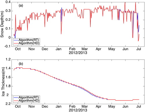
The algorithm has two modules. One is designed to process historical archived SIMBA data (HD), and the other one is targeted to process online near real-time SIMBA data (RT). The RT requires the algorithm to be operated repeatedly on a daily basis as long as the SIMBA buoy is still working. This means that once new SIMBA data comes in, instead of processing the new temperature data, the RT algorithm will process the entire time series of SIMBA data that was obtained from the beginning of measurement to the current date. Such a procedure is necessary to avoid numerical instability of the snow surface created by the uncertainty in the first guess of the initial sensor position predefined by the algorithm at each time step. If the algorithm cannot identify the snow surface and ice bottom on a current day, the result of the previous day will be used as the first guess values for the next day. Ideally, these two modules should provide the same results. One test trial for buoy A suggested that the snow depth estimation had a few spike-point differences between the HD and RT modules. Although the differences can be as large a 20 cm (Figure 8(a)), the differences do not impact overall result as a whole. The ice thickness derived by both modules were close to each other (Figure 8(b)). The thickness difference was confined to 2–4 cm (1–2 sensor intervals). For the RT module, the repeating operation may sometimes require many iteration times and the time efficiency of the algorithm may be reduced. There is still a need for a better alternative for operation of the algorithm in real-time snow depth and ice thickness detection.

Figure 8. Time series of snow depths and ice thicknesses retrieved by the algorithm using historical data (HD) and online real-time data (RT).

3.4. Thermodynamic modeling of snow depth and ice thickness

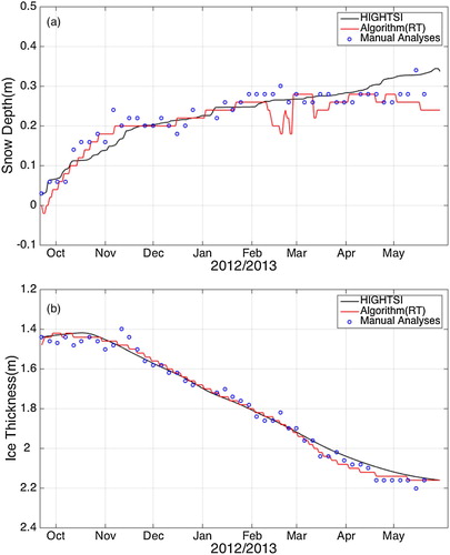
The SIMBA buoys are often deployed on a drift ice floe or at a fixed location on landfast sea ice. Hence, changes in snow depth and ice thickness are largely in response to atmospheric conditions and dominated by the thermodynamic processes along the buoy drift trajectories or at the fixed location. Snow depth and ice thickness along buoy drift trajectories or at a fixed location can be simulated using a thermodynamic sea ice model (Merkouriadi et al. 2017; Tian et al. 2017; Zhao et al. 2017). Such a modelling experiment was performed for buoy A. The aim was to see how snow depth and ice thickness can be reproduced using a physical model, and whether or not the temperature (thermodynamics)-derived snow and ice mass balances would be consistent with the model results. A high-resolution 1-D snow/ice thermodynamic model (HIGHTSI) was used to calculate snow depth and ice thickness. HIGHTSI is a process model used to accurately resolve the evolution of snow/ice thickness and the temperature profile (Launiainen and Cheng 1998; Cheng et al. 2008). In this study, the external weather forcing variables for HIGHTSI were taken from operational analyses and short-term forecasts from the European Centre for Medium-Range Weather Forecasts (ECMWF) numerical weather prediction (NWP) model and SIMBA measurements. The variables were air temperature at a 1  m height above the snow surface (SIMBA observations), dew-point temperature, 10  m wind speed, total cloud cover, downward solar shortwave and thermal longwave radiative fluxes, and snow precipitation. The parameters based on the ECMWF products were interpolated along the buoy drift trajectory. The model simulation covered the period from 21 September 2012 to 30 May 2013. The initial snow depths and ice thicknesses were taken from buoy measurements. The SIMBA based and HIGHTSI simulated snow depths and ice thicknesses are shown in Figure 9. The algorithm obtained decreasing snow depths in late February and mid-March, which differ from the results of other methods. From late April onward, the modelled snow depth was still increasing, while the SIMBA buoy suggested that the increase of snow depth had stopped. The decreasing of snow depth in an Arctic winter is most likely associated with snow drift. The modelled snow depth showed weak temporal variation compared with SIMBA data analyses because snow drift was not taken into account in the model. Overall, an increase of snow depth was revealed by both SIMBA data analyses and HIGHTSI model calculation during most of the study period between late September and early April. The total ice thickness provided using these methods were in good agreement. The HIGHTSI produced a comparable ice thickness evolution along the buoy drift path. Note the model simulation here applied SIMBA near-surface air temperature as forcing. If we use ECMWF 2  m air temperature instead, the modelled ice thickness would be approximately 15% less by the end of the simulation. The air temperature is critical to sea ice mass balance on a seasonal scale. In this case, the modelling results were able to fill the gaps of the missing SIMBA observations.

Figure 9. Snow depths and ice thicknesses derived from the SIMBA temperature field using manual analyses (dots), SIMBA HD-algorithm (grey line), and HIGHTSI model simulation (black line).

3.5. Discussion

A comparison between algorithm based, manually derived, and in situ observed snow depths and ice thicknesses is summarized in Table 2.

Table 2. Comparison between manually derived in situ observed and algorithm-based snow depths and ice thicknesses. The manually derived and in situ observed results were used as the reference values to calculate the bias and root-mean-squared error (RMSE).

SIMBA buoy			Algorithm (AI)	Manual (Ma)
A	Total thickness (cm)	Mean	200.5	200.7
		Standard deviation	31.7	32.2
		Bias (Al-Ma)	–1.5
		RMSE	10.5
		Corr. coefficient	0.99
	Snow depth (cm)	Mean	21.5	22.7
		Standard deviation	6.5	6.9
		Bias	–1.6
		RMSE	10.6
		Corr. coefficient	0.90
	Ice thickness (cm)	Mean	179.0	178.0
		Standard deviation	26.6	26.7
		Bias	1.2
		RMSE	2.4
		Corr. coefficient	0.99
B	Total thickness (cm)	Mean	162.9	161.4
		Standard deviation	2.7	6.3
		Bias (Al-Ma)	1.4
		RMSE	4.3
		Corr. coefficient	0.95
	Snow depth (cm)	Mean	40.7	41.4
		Standard deviation	1.9	2.4
		Bias	–0.7
		RMSE	0.7
		Corr. coefficient	0.96
	Ice thickness (cm)	Mean	122.1	120.0
		Standard deviation	2.7	5.8
		Bias	2.1
		RMSE	3.6
		Corr. coefficient	0.95
			AI	In situ Ob.
C	Ice thickness (cm)	Mean	139	136
		Standard deviation	35	34
		Bias	2.5
		RMSE	8.9
		Corr. coefficient	0.99

For Buoy A and B, the average total thickness (snow depth + ice thickness) obtained using the algorithm and by manual analyses are very close to each other. The difference is less than 1 cm. The average snow depth and ice thickness between algorithm-based and manually derived results are close to each other. The bias and RMSE between algorithm and manually derived total thickness range from –1.5 cm to 1.4 cm and 10.5 cm to 4.3 cm, respectively. For snow depth, the corresponding ranges are from –0.7 cm to 1.6 cm and 0.7 cm to 11 cm, respectively. For ice thickness, the values are from 1.2 cm to 2.1 cm and from 2.4 cm to 3.6 cm, respectively. The bias of snow depth and ice thickness estimation between the algorithm and the manual analyses was roughly 2%–7% of the total mean snow depth and 1%–2% of the total mean ice thickness, respectively. The algorithm and manual results agreement are better for ice thickness than for snow depth. For buoy C, the difference between the algorithm based and in situ observed mean ice thickness is 3 cm. The bias and RMSE are 2.5 cm and 8.9 cm, respectively. The bias is about 2% of the total mean ice thickness. The algorithm provided quite good results compared with in situ observations for the bare ice condition. The RMSE between the algorithm and the manual in situ observed ice thicknesses ranged from 2.4 cm to 8.9 cm, accounting for 2%–7% of the total mean ice thickness.

The thermistor chain has 240 sensors. Usually 50–60 sensors are mounted vertically above the surface in the air. This would allow for a maximum of 100–120 cm of snow accumulation. The remaining 180 sensors covered a depth of 360 cm and were distributed in the ice and in the ocean. It is important to preserve a high enough number of sensors in the air (Tian, personal communication). A short segment of the thermistor string placed in the air might cause in-air senior chain segment to be entirely buried below the snow, which can lead to a complete failure of the algorithm because the algorithm would not be able to identify the first guess value for the top surface position.

The algorithm treated snow/ice interface was used as the reference level. Once the top and bottom positions were identified, the snow depth and ice thickness were distances from the reference level to the top and bottom sensor positions, respectively. In practice, the snow/ice interface may not be at a fixed position. In early winter when ice is thin, heavy snowpack on ice contributes to the ice mass due to widespread surface flooding and snow-ice formation (Leppäranta 1983). During the melting season, refreezing of melted snow often results in superimposed ice formation at the snow/ice interface (Kawamura et al. 1997; Nicolaus et al. 2003). These processes could actively alter the position of the snow/ice interface. A SIMBA deployed in an Arctic lake suggested that the snow/ice interface was moving upward in response to snow-ice formation (Cheng et al. 2014). In the Arctic Ocean, ice mass balance buoys (IMBs) have been deployed on thick under-formed multi-year sea ice floes to ensure long-life operation. Onsite sea ice is often more than 2  m thick, creating strong buoyancy to prevent any snow-ice formation. The buoys are often deployed during the Arctic autumn when the melting season will soon stop. The superimposed ice formation will contribute a minimal effect on the movement of the snow/ice interface. Accordingly, a fixed snow/ice interface reference level is a feasible assumption for a buoy algorithm.

Data was processed successfully from ten SIMBA buoys. Most of them were deployed in the Arctic. So far, algorithm operations have been restricted to the cold season to ensure reliable results. This is because, during the melting season (July–August in the Arctic), the in-ice temperature gradient at the ice base may be too small due to the impact of brine channels, thereby creating a skeleton layer. This can lead to an underestimation of the total ice thickness.

A 30-cm maximum daily snow snowfall or ablation and 10-cm daily maximum ice bottom growth or ablation were assumed threshold values based on field measurements in the Arctic Ocean. These are reasonable values to be used in this algorithm. Tuning these values will affect top and bottom positions. When compared with heating temperature, the discriminated air/snow interface increasing or decreasing upper threshold values may result in thicker or thinner snow depth, respectively. The sensitivity of the lower threshold value to the identified ice thickness was weak, but the algorithm may have no result if the daily maximum bottom ice growth or ablation is too small. Therefore, 2 cm was assumed for the threshold value.

The temperature differences between adjoined sensors for buoy A are illustrated in Figure 10. According to Equation (10), a large part of the area above the 0 level in Figure 10(a) was evidently snow. The color shadow area in Figure 10(b) represents the sea ice. The discriminated horizontal line approximately 0.22  m below the 0 reference level in (b) is actually the sea water level in the thermistor string borehole (Figure 6(a) while broken line). The area identified by the temperature differences (0.1875≤ | ΔT | ≤ 0.4375) between 0 and –0.22  m may refer to a mixture of snow and ice. During June and July, the upper snow is likely getting wet in response to surface melt, and the signal of the snow/ice mixture is stronger.

Figure 10. Time series of temperature differences between adjoined sensors in the snow and ice for buoy A. Temperature differences larger than 0.4375°C were excluded in (a), while temperature differences larger than 0.1875°C were excluded in (b). The minimum temperature difference in (a) and (b) is 0.0625°C.

4. Conclusions

The SIMBA device is a recent development of the IMB. It measures high spatial resolution vertical temperature profiles through the air–snow–sea ice–ocean column using a thermistor string with a standard configuration of 240 sensors at 2 cm spacing. The snow depth and ice thickness are often obtained manually from visual inspection of temperature gradients in air, snow, ice and water. The SIMBA unit also offers a heating mode to assist in identification of the surrounding media and interfaces. In this study, an automated algorithm has been developed to retrieve snow depth and ice thickness from SIMBA temperature profiles.

The algorithm is based on the heat flux continuation between adjoined layers in snow and ice. The ratio between thermal heat conductivity of snow and ice are used to identify temperature patterns between adjoined layers in snow and ice. The temperature resolution of ± 0.0625°C for SIMBA thermistor string is also critical in connection with an identified temperature gradient in snow and ice. The algorithm works automatically once a few input parameters are defined. The algorithm has two modules, which can be used to process historical and operational online real-time SIMBA data. For the latter one, the operational procedure would require multiple iterations and the efficiency of the algorithm still needs to be improved. Our tests indicate both modules yield similar results.

The heating mode of SIMBA is useful for identifying top air/snow and bottom ice/ocean interfaces, particularly in isothermal conditions. However, the interface discrimination may become poor in some conditions which prevent the determination of snow depth and ice thickness from SIMBA data. The algorithm yielded results that are comparable with manual analyses and in situ measurements. The agreement is better for ice thickness retrieval than for snow depth. The algorithm provides a good result for bare ice conditions.

The snow/ice interface (i.e. the ice surface) is assumed as a reference level and remains unchanged. This criterion is also applied for CRREL IMB (Richter-Menge et al. 2006). This criterion is feasible for a thick ice floe. A recent study by Provost et al. (2017) suggested, however, that the snow/ice interface could move upward in response to the snow-ice formation during Arctic winter where a SIMBA was deployed on a 1.5  m ice with 0.5  m thick snow. So far our algorithm cannot identify a moving snow/ice interface. If such conditions are present then additional manual analyses are needed to identify a reliable snow/ice interface.

Challenges still remain for making the algorithm reliable when applied to warm conditions. During the melting season (August–September in the Arctic), the in-ice temperature gradient at the ice base may be too small due to the impact of brine channels creating a skeleton layer leading to an underestimation of the total ice thickness.

More case studies, preferably with in situ manual thickness measurements, would be needed in order to further test algorithm performance under different thermodynamic conditions. Another possibility would be to add acoustic sounder as a supplemental component of SIMBA (Lei et al. 2018) so that the algorithm results can be compared with a thickness measured by sounders. Reliable buoy data can also be used to validate numerical sea ice models. On the other hand, the modelling results can fill the gap of missing buoy measurements, especially for the melting period, when buoy measurements may be liable to large errors (Tian et al. 2017).

The IMB is a valuable instrument for monitoring snow depth and ice thickness in the Polar oceans. The cost-cutting design of the SIMBA buoy makes it possible to deploy a large array in investigations of regional and large-scale sea ice mass balance. A reliable SIMBA algorithm would be a very useful tool for improving the consistency and repeatability of data interpretation across the IMB buoy network which is an important component of the Integrated Arctic Observation System.

Acknowledgments

The authors are grateful for the SIMBA deployment made by our international collaborators. The FMI02 was deployed by Dr. Marcel Nicolaus from AWI in autumn 2012; FMI20 was deployed during the NICE2015 field campaign. NMEFC-Ant2014 was deployed by Mr. Xiaopeng Han from NMEFC in autumn 2014.

Disclosure statement

No potential conflict of interest was reported by the authors.

Additional information

Funding

This work was supported by Academy of Finland [grant number 317999], Natural Science Foundation of China [grant numbers 41376005, 41406218, 41428603, 41506221, 11571383], European Union’s Horizon 2020 research and innovation programme [No 727890 – INTAROS], the Key Research Program of Frontier Sciences of CAS [QYZDY-SSW-DQC021] and the Science and Technology Program Guangzhou, China [201804020053].

References

- Cheng, B., T. Vihma, L. Rontu, A. Kontu, P. H. Kheyrollah, C. Duguay and J. Pulliainen. 2014. “Evolution of Snow and Ice Temperature, Thickness and Energy Balance in Lake Orajärvi, Northern Finland.” Tellus A 66: 21564. http://doi.org/10.3402/tellusa.v66.21564.
- Cheng, B., Z. Zhang, T. Vihma, M. Johansson, L. Bian, Z. Li, and H. Wu. 2008. “Model Experiments on Snow and Ice Thermodynamics in the Arctic Ocean with CHINARE 2003 Data.” Journal of Geophysical Research Oceans 113(9): 1–15.
- Döscher, R., T. Vihma, and E. Maksimovich. 2014. “Recent Advances in Understanding the Arctic Climate System State and Change From a Sea ICE Perspective: A Review.” Atmospheric Chemistry and Physics 14: 13571–13600. doi: 10.5194/acp-14-13571-2014
- Granskog, M. A., P. Assmy, S. Gerland, G. Spreen, H. Steen, and L. H. Smedsrud. 2016. “Arctic Research on Thin Ice: Consequences of Arctic Sea Ice Loss.” EOS Transactions American Geophysical Union 97(5): 22–26.
- Hoppmann, M., M. Nicolaus, P. A. Hunkeler, P. Heil, L. K. Behrens, G. König-Langlo, and R. Gerdes. 2015. “Seasonal Evolution of an Ice-Shelf Influenced Fast-Ice Regime, Derived From an Autonomous Thermistor Chain.” Journal of Geophysical Research: Oceans 120: 1703–1724.
- Itkin, P., G. Spreen, B. Cheng, M. Doble, F. Girard-Ardhuin, J. Haapala, N. Hughes, L. Kaleschke, M. Nicolaus, and J. Wilkinson. 2017. “Thin Ice and Storms: Sea Ice Deformation From Buoy Arrays Deployed During N-ICE2015.” Journal of Geophysical Research Oceans 122(6): 4661–4674. doi: 10.1002/2016JC012403
- Jackson, K., J. Wilkinson, T. Maksym, D. Meldrum, J. Beckers, C. Haas, and D. Mackenzie. 2013. “A Novel and Low Cost Sea Ice Mass Balance Buoy.” Journal of Atmospheric and Oceanic Technology 30(11): 2676-2688. doi: 10.1175/JTECH-D-13-00058.1
- Kawamura, T., K. I. Ohshima, T. Takizawa, and S. Ushio. 1997. “Physical, Structural, and Isotopic Characteristics and Growth Processes of Fast Sea Ice in Liitzow-Holm Bay.” Journal of Geophysical Research Oceans 102(C2): 3345–3355. doi: 10.1029/96JC03206
- Kwok, R., G. F. Cunningham. 2015. “Variability of Arctic Sea Ice Thickness and Volume From CryoSat-2.” Philosophical Transactions of the Royal Society A 373(2045): 20140157-–20140157. doi: 10.1098/rsta.2014.0157
- Launiainen, J., and B. Cheng. 1998. “Modelling of ice Thermodynamics in Natural Water Bodies.” Cold Regions Science and Technology 27(3): 153–178. doi: 10.1016/S0165-232X(98)00009-3
- Laxon, S. W., K. A. Giles, A. L. Ridout, D. J. Wingham, R. Willatt, R. Cullen, and R. Kwok et al. 2013. “CryoSat-2 Estimates of Arctic Sea Ice Thickness and Volume.” Geophysical Research Letters 40: 732–737. doi:10.1002/grl.50193.
- Lei, R., B. Cheng, P. Heil, T. Vihma, J. Wang, Q. Jiand, and Z. Zhang. 2018. “Seasonal and Interannual Variations of Sea Ice Mass Balance From the Central Arctic to the Greenland Sea.” Journal of Geophysical Research Oceans 123: 2422–2439. doi:10.1002/2017JC013548.
- Leppäranta, M. 1983. “A Growth Model for Black ice, Snow Ice and Snow Thickness in Subarctic Basins”, Nordic Hydrology 14, 59–70. doi: 10.2166/nh.1983.0006
- Merkouriadi, I., B. Cheng, M. Graham, A. Rösel, M. A. Granskog. 2017. “Critical Role of Snow on Sea Ice Growth in the Atlantic Sector of the Arctic Ocean.” Geophysical Research Letters 44 (20):10479-10485. doi: 10.1002/2017GL075494
- Nicolaus, M., C. Haas, and J. Bareiss. 2003. “Observations of Superimposed Ice Formation at Melt-Onset on Fast ice on Kongsfjorden, Svalbard.” Physics and Chemistry of the Earth 28: 1241–1248. doi: 10.1016/j.pce.2003.08.048
- Overland, J., E. Hanna, I. Hanssen-Bauer, S. J. Kim, J. Walsh, M. Wang, and U.S. Bhatt. 2016. “Arctic air Temperature [In State of the Climate in 2015].” The Arctical Bulletin of the American Meteorological Society, 97(8): S132–S134.
- Overland, J. E., K. R. Wood, and M. Wang. 2011. “Warm Arctic - Cold Continents: Climate Impacts of the Newly Open Arctic Sea.” Polar Research 30: 157-171. doi: 10.3402/polar.v30i0.15787
- Parkinson, C. L, and W. M. Washington. 1979. “A Large-Scale Numerical Model of Sea Ice.” Journal of Geophysical Research 84(C1): 311–337. doi: 10.1029/JC084iC01p00311
- Perovich, D. K., T. C. Grenfell, J. A. Richter-Menge, B. Light, W. B. Tucker, and H. Eicken. 2003. “Thin and Thinner: Sea ice Mass Balance Measurements During SHEBA.” Journal of Geophysical Research 108 (C3): 8050, doi:10.1029/2001JC001079.
- Perovich, D. K., and J. A. Richter-Menge. 2015. “Regional Variability in Sea Ice Melt in a Changing Arctic.” Philosophical Transactions of the Royal Society A-Mathematical Physical Engineering Science 373(2045): 20140165. doi: 10.1098/rsta.2014.0165
- Pringle, D. J., H. Eicken, H. J. Trodahl, and L. G. E. Backstrom. 2007. “Thermal Conductivity of Land Fast Antarctic and Arctic sea ice.” Journal of Geophysical Research 112: C04017, doi:10.1029/2006JC003641.
- Provost, C. N. Sennechael, J. Miguet, P. Itkin, A. Röosel, Z. Koenig, N. Villacieros-Robineau, and M. A. Granskog. 2017. “Observations of Flooding and Snow-Ice Formation in a Thinner Arctic Sea-Ice Regime During the N-ICE2015 Campaign: Influence of Basal Ice Melt and Storms.” Journal of Geophysical Research: Oceans 122: 7115–7134. doi:10.1002/2016JC012011.
- Richter-Menge, J. A., D. K. Perovich, B. C. Elder, K. Claffey, I. Rigor, and M. Ortmeyer. 2006. “Ice Mass Balance Buoys: A Tool for Measuring and Attributing Changes in the Thickness of the Arctic Sea-Ice Cover.” Annals of Glaciology 44: 205–210. doi: 10.3189/172756406781811727
- Rösel, A., C. M. Polashenski, G. E. Liston, J. A. King, M. Nicolaus, J. C. Gallet, and D. Divine, et al. 2016. N-ICE2015 Snow Depth Data with Magnaprobe [Data Set]. Tromsø: Norwegian Polar Institute. doi:10.21334/npolar.2016.3d72756d.
- Sturm, M., J. Holmgren, M. König, and K. Morris. 1997. “The Thermal Conductivity of Seasonal Snow.” Journal of Glaciology 43: 26–40. doi: 10.1017/S0022143000002781
- Thomas, D. N. and Dieckmann, G. S. eds. 2008. Sea Ice: An Introduction to its Physics, Chemistry, Biology, and Geology. Oxford: Blackwell Science.
- Tian, Z., B. Cheng, J. Zhao, T. Vihma, W., Zhang, Z., Li and Z., Zhang. 2017. “Observed and Modelled Snow and ice Thickness in the Arctic Ocean with CHINARE Buoy Data.” Acta Oceanologica Sinica 36(8): 66–75. doi: 10.1007/s13131-017-1020-4
- Vihma, T. 2014. “Effects of Arctic sea ice Decline on Weather and Climate: A Review.” Surveys in Geophysics 35: 1175–1214. doi:10.1007/s10712-014-9284-0.
- Warren, S. G., I. G. Rigor, N. Untersteiner, V. E. Radionov, N. N. Bryazgin, Y. I. Aleksandrov, R. Colony. 1999. “Snow Depth on Arctic Sea Ice.” Journal of Climate 12(6): 1814-1829. doi: 10.1175/1520-0442(1999)012<1814:SDOASI>2.0.CO;2
- Yen, Y.-C. 1981. Review of thermal properties of snow, ice and sea ice. Cold Region Research and Engineering Laboratory Hanover New Hampshire Report ADA103734.
- Zhang, Z. ed. 2004. The Report of 2003 Chinese Arctic Research Expedition. Beijing: China Ocean Press.
- Zhao, J., Q. Yang, B. N. Wang, F. Hui, H. Shen, X. Han, L. Zhang and T. Vihma. 2017. “Snow and Land-Fast Sea Ice Thickness Derived From Thermistor Chain Buoy in the Prydz Bay, Antarctic” Acta Oceanologica Sinica in Chinese 39(11):115–127. doi: 10.3969/j.issn.0253-4193.2017.11.011