Increasing the detail of European land use/cover data by combining heterogeneous data sets

ABSTRACT

Data on land use and land cover (LULC) are a vital input for policy-relevant research, such as modelling of the human population, socioeconomic activities, transportation, environment, and their interactions. In Europe, CORINE Land Cover has been the only data set covering the entire continent consistently, but with rather limited spatial detail. Other data sets have provided much better detail, but either have covered only a fraction of Europe (e.g. Urban Atlas) or have been thematically restricted (e.g. Copernicus High Resolution Layers). In this study, we processed and combined diverse LULC data to create a harmonised, ready-to-use map covering 41 countries. By doing so, we increased the spatial detail (from 25 to one hectare) and the thematic detail (by seven additional LULC classes) compared to the CORINE Land Cover. Importantly, we decomposed the class ‘Industrial and commercial units’ into ‘Production facilities’, ‘Commercial/service facilities’ and ‘Public facilities’ using machine learning to exploit a large database of points of interest. The overall accuracy of this thematic breakdown was 74%, despite the confusion between the production and commercial land uses, often attributable to noisy training data or mixed land uses. Lessons learnt from this exercise are discussed, and further research direction is proposed.

KEYWORDS:

• Data fusion
• land use
• land cover
• machine learning
• points of interest

1. Introduction

Land use and land cover (LULC) maps provide information about the bio-physical cover of the Earth surface and the purposes for which humans exploit it (Verburg et al. 2009). Detailed, harmonised and up-to-date LULC information is crucial, for example, in Earth system and socioeconomic sciences, evidence-based planning at multiple levels of governance, and policies targeting sustainable development goals (Ben-Asher et al. 2013). In Europe, CORINE Land Cover (CLC) data has been widely used as the reference LULC dataset, for instance to estimate carbon stored in vegetation (Cruickshank, Tomlinson, and Trew 2000), to interpolate air-pollution mesurements (Janssen et al. 2008), to analyse urban heat islands (Stathopoulou and Cartalis 2007), and to disaggregate population counts (Gallego et al. 2011). CLC is a unique and valuable series of harmonised Europe-wide datasets spanning four temporal horizons (1990, 2000, 2006, and 2012). Three layers identifying changes of LULC have been produced so far covering periods of 1990–2000, 2000–2006, and 2006–2012 (Büttner 2014). While the CLC’s name refers only to land cover, its nomenclature comprises 19 land use and 25 cover classes (Fisher, Comber, and Wadsworth 2005), organised in a three-tier hierarchical system. Bossard, Feranec, and Oťaheľ (2000) have provided a comprehensive description of the nomenclature.

Despite its merits, some limitations of CLC in specific applications have been noted (Schmit, Rounsevell, and La Jeunesse 2006; Diaz-Pacheco and Gutiérrez 2014). The high number of thematic classes in the nomenclature does not guarantee its versatility. Most analyses that focus on human-environment interaction would benefit from a more detailed classification of artificial and agricultural areas while the breakdown of forests, semi-natural, wetland and water areas could be less detailed. Modelling of population distribution requires a finer land use distinction of artificial surfaces, to which people are bound at almost all times. Daytime population modelling is especially challenging, as it demands the knowledge of areas used for employment, transport, leisure, education, and other activities. In the context of CLC, a major knowledge gap could be bridged by classifying the heterogeneous class Industrial or commercial units (ICU) into subclasses matching economic sectors, for which employment statistics are available.

Other limitations of CLC are related to the spatial detail and cartographic representation. At the time of CLC’s launch in the late 1980s, the manual mapping approach and relatively coarse resolution of available Earth observation data allowed for mapping of areas having at least 25 ha in area and 100 m in width. Such a generalised model of landscape underrepresents especially land use categories occurring in rather smaller patches (e.g. various kinds of artificial surfaces) and can hardly capture the fine-grained nature of economic activities, especially in an urban setting (Jokar Arsanjani, See, and Tayyebi 2016). For instance, as pointed out by Gallego et al. (2011), a large share of local administrative units (municipalities) in Europe did not contain any built-up area larger than 25 ha. The insufficient spatial detail hence limits the application of CLC for land accounting, population distribution modelling and land use change modelling, among other uses.

In the last decade, new Europe-wide geodata sources have emerged, that could potentially alleviate some of the limitations. These include public sources such as the European Union (EU) Copernicus programme, proprietary data as well as volunteered geographic information. In brief, currently available data on land cover, land use and economic activities are richer and more detailed than ever but fragmented in a variety of data sources, types and formats. We propose to expand the knowledge base of European LULC by integrating part of the multitude of currently available geo-datasets within the widely used CLC framework in a consistent manner. The result should have a superior spatial detail compared to CLC, which can better accommodate further improvements introduced in the thematic domain. The ultimate aim of the improved EU-wide LULC data is to enable better support for socioeconomic and geographic inquiries, such as modelling of the human population, economic activity, land use, transportation, environment and their interaction. Given the spatial extent and resolution of the data, the output of this work is relevant for models constructed at continental, national or regional scale.

The remainder of this article is structured as follows: Section 2 refers previous works on the topic; Section 3 describes the data and methods used, divided into two main parts – the spatial and the thematic refinement; Section 4 previews the results, evaluates their quality and compares them to CLC; Section 5 discusses the results, limitations and directs possible future research; Section 6 concludes the whole work.

2. Related works

Spatial refinements of a pre-existing LULC map have been described in the literature, although the examples are rather scarce. Batista e Silva, Lavalle, and Koomen (2013) have refined CLC2006 with multiple ancillary datasets at the European level as have done Pazúr and Bolliger (2017) with CLC2012 but only for Slovakia. Stewart (1998) refined a remote sensing derived LULC map with ancillary data for a study area in Wisconsin, and Fonte et al. (2017) have demonstrated the refinement of GlobeLand30 with OpenStreetMap (OSM) land use data for small study areas (Kathmandu, Dar es Salaam). The methodology differed from study to study to accommodate the characteristics of the employed datasets. While the former two studies incrementally added data to the CLC and tried to keep the original CLC legend, the latter two involved an element of thematic refinement too. A similar data fusion work has been demonstrated by Schultz et al. (2017) who have used OSM land use polygons to train a machine learning classifier of satellite imagery. The classified image was used to fill gaps not covered by OSM, generating a seamless LULC map at the second level of CLC legend for the Heidelberg area, Germany.

Thematic enhancement per se has been addressed by Theobald (2014) who has derived a detailed land use classification for the United States by fusing land cover map with multiple disparate types of data. Jiang et al. (2015) have derived activity levels per refined economic sectors at census block level by mining information from proprietary and volunteered databases of points of interest (POI). Yao et al. (2017) have used POI to derive urban land uses per traffic analysis zones. Similarly, information from POI has been used to semantically enrich building footprint data (Kunze and Hecht 2015). Other researchers have characterised LULC, human activites and place semantics using social sensing (Liu et al. 2015). The employed data range from spatio-temporal mobile phone data (Jacobs-Crisioni et al. 2014; Pei et al. 2014; Ríos and Muñoz 2017), Foursquare data (Aubrecht et al. 2017; Spyratos et al. 2017), geotweets (Frias-Martinez and Frias-Martinez 2014; Lloyd and Cheshire 2017), and georeferenced photos (Feick and Robertson 2015; Antoniou et al. 2016). Each of the social sensing approaches presents a considerable challenge for pursuing at a continental scale, due to data access, computational demand, or spatially and demographically biased user bases. Hence the above mentioned case studies were typically spatially restricted to the city level.

3. Data and methods

In this section, we describe the data, assumptions and methodology to produce a refined map by integrating a series of datasets with CLC for the reference year 2012. The study area covers the 28 EU members, Iceland, Liechtenstein, Norway, and Switzerland (EFTA), Western Balkans countries, and Turkey (Figure 6). It includes the Azores, Canary Islands, Madeira, but excludes Andorra, Faroe Islands and the French overseas territories.

The suggested workflow comprises of two main domains (Figure 1). First we modify the CLC 2012 map by including a set of datasets with superior spatial resolution (Table 2). The increase of spatial detail from 25 to 1 hectar (5 ha for non-artificial classes outside of urban areas) provides the foundation for subsequent thematic refinement of the 11 classes of Artificial surfaces into 18 classes (Table 1), leading to a total of 50 classes in the final result. The original CLC legend and proposed expanded legend are provided in Figure 2 as a reference for other figures throughout the article.

Figure 1. A simplified data processing flowchart.

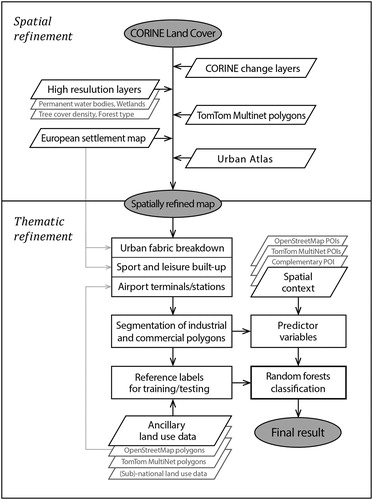
Figure 2. The original and refined colour-code matching used throughout the article.

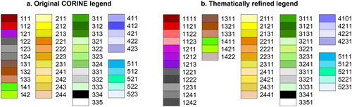
Table 1. The target legend of the artificial classes expanded into the fourth hierarchical level (dark grey fill – classes expanded, light grey fill – classes not-changed).

CLC1	CLC2	Level 2 Label	CLC3	Level 3 Label	CLC4	Level 4 Label
1 Artificial surfaces	11	Urban fabric	111	Continuous urban fabric	1111	Urban fabric high density
			112	Discontinuous urban fabric	1121	Urban fabric medium density
					1122	Urban fabric low density
					1123	Urban fabric very low density/isolated
	12	Industrial, commercial and transport units	121	Industrial and commercial units	1211	Production facilities
					1212	Commercial/service facilities
					1213	Public facilities
			122	Road or rail networks and associated land	1221	Road/rail networks and associated land
					1222	Major stations
			123	Port areas	1231	Port areas
			124	Airport areas	1241	Airport areas
					1242	Airport terminals
	13	Mines, dumps and construction sites	131	Mineral extraction sites	1311	Mineral extraction sites
			132	Dump sites	1321	Dump sites
			133	Construction sites	1331	Construction sites
	14	Artificial vegetated non-agricultural areas	141	Green urban areas	1411	Green urban areas
			142	Sport and leisure facilities	1421	Sport and leisure green
					1422	Sport and leisure built-up

3.1. Spatial refinement

The presented approach elaborates on the methodology proposed by Batista e Silva, Lavalle, and Koomen (2013) for the production of the 2006 refined LULC map and introduces several updates to maximise mining useful information from data available for 2012. The EU Copernicus programme provides monothematic high-resolution layers (HRL) and detailed data from the Urban Atlas (UA) programme. The set of urban areas (so called Larger Urban Zones) included in UA2012 doubled compared to the 2006 release. The UA’s thematic resolution improved moderately too, easing its fusion with CLC (European Commission 2011, 2016). Another novel dataset highly relevant for the refinement of CLC is the European Settlement Map (ESM, Ferri et al. 2014), a product related to the Global Human Settlement Layers (Pesaresi et al. 2016). It is an innovative dataset capturing built-up areas from high resolution satellite imagery (2.5 m pixel size).

The spatial refinement relied on the cartographic synthesis of categorical raster data, interval raster data, and vector polygon data. The data fusion was performed using an automated chain of raster-based map algebra operations (Tomlin 1990) on a set of raw or pre-processed datasets. Input vector data were rasterised to the target 100 m resolution beforehand, using the maximum combined area method to identify the dominant class in each cell. At each step of the sequence, the cells either remained unchanged or were updated by the overlaid input data layer, following pre-established decision rules. We present an overview of the individual steps in Table 2 and a more detailed description in the following subsections.

Table 2. Specification of the datasets included in the spatial refinement (Sections 3.1.1. to 3.1.7), a simplified description of the fusion rules applied and classes directly affected.

Section	Input data source	Ref. year	Spatial detail	Data model	Rules for including	Affected classes
-	CORINE land cover status	2012	25 ha	Vector	The background layer	All
3.1.1.	CORINE land cover change	2006–2012	5 ha	Vector	Changes 2006–2012: all change polygons available Changes 2000–2006: changes to artificial classes or at 1st–2nd level, 5–25 ha	All
3.1.2.	High resolution layer Tree cover density	2012	100 × 100 m	Raster	Minimum 5 contiguous pixels with value > 50% tree cover	311, 312, 313
	High resolution layers Water bodies, Wetlands	2012	100 × 100 m	Raster	Minimum 5 contiguous pixels with value > 50% combined cover of wetland and water	4XX, 51X
3.1.3.	TomTom MultiNet Land Use polygons	2013	N/A	Vector	Categories corresponding to industrial, commercial, transport and green urban areas selected; polygons represented by at least one cell after rasterization included.	121, 122, 123, 124, 141, 142
3.1.4.	European Settlement Map (2016 release)	2012	100 × 100 m	Raster	Individual pixels with >5% built-up cover. Changes in non-residential artificial classes are restricted.	11X
3.1.5.	Urban Atlas	2012	0.25/1 ha	Vector	All polygons represented by at least one cell after rasterization are included. A decision matrix (original CORINE class vs Urban Atlas class) determined the final classification of overlapping pixels.	All
3.1.6.	TomTom MultiNet Built-up polygons	2013	N/A	Vector	About 1% of municipalities, for which the amount of built-up is significantly lower than expected (given an empirical relationship between size of the population and urban fabric surface) refined by adding built-up areas from TomTom	112
3.1.7.	OpenStretMap roads, TomTom tunnels	2013	N/A	Vector	Motorways and major national roads rasterised, tunnel segments masked out. Replace all classes; except: artificial classes replaced only if ESM built-up cover < road cover	122
	River mask (HRL Water bodies)	2012	N/A	Raster	River features extracted based on linear appearance. Replace all classes; except: artificial classes replaced only if ESM built-up cover < HRL water cover	511

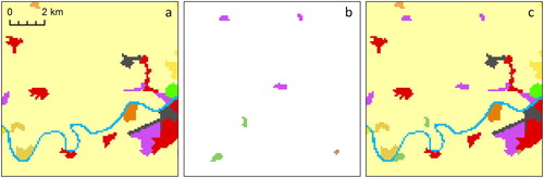
3.1.1. CLC change maps

The CLC change maps comprise LULC change patches as small as 5 ha. These are combined with the previous status layer to produce the updated status layer. Due to generalisation rules (EEA 2007, 18), some of the smaller change patches are not transferred into the status layer. We recovered this unexploited detail by including the output value of the disregarded change patches (Figure 3). We included all patches from the 2006–2012 change layer and a selection of relevant patches (i.e. changes resulting in artificial surfaces or changes between first/second level classes) from the 2000–2006 change layer. Patches smaller than five and larger than 25 ha were excluded (patches in this size range not transferred to the status layer 2006 tended to be false changes).

Figure 3. Including the CORINE Land Cover change polygons (a. previous state, b. update data, and c. result; the same layout applies to Figures 4–6 and 8–11). Legend is provided in Figure 2(a).

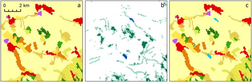
3.1.2. Copernicus high resolution layers

Further, we employed the available Copernicus HRL. The layers are produced from satellite imagery at 20 m spatial resolution by a semi-automatic method. The cell values represent the intensity of the individual land cover, ranging from 0 to 100% (Langanke et al. 2016). We used the aggregated 100 m versions of HRL Tree cover Density, HRL Wetlands, and HRL Permanent Water Bodies. We did not consider two other available layers: HRL Natural grasslands as it had a one-to-many relationship with CLC classes; and HRL Imperviousness, which was superseded by the ESM dataset. We applied 50% threshold to extract areas in which the respective class is likely to be dominant (Figure 4) and reduced noise by retaining only contiguous groups of at least five contiguous cells (rook contiguity). Another HRL, Forest Type, was used to derive a third-level class of the included forest patches (broadleaved, coniferous, mixed).

Figure 4. Including new forest and water patches based on Copernicus high resolution layers. Green shades in the box b represent forest and blue shades represent water areas. Cells above 50% threshold (represented by the more saturated shade) and in groups of minimum five were extracted. Legend for boxes a and c is provided in Figure 2(a).

3.1.3. Tomtom Multinet 2014 – land use layer

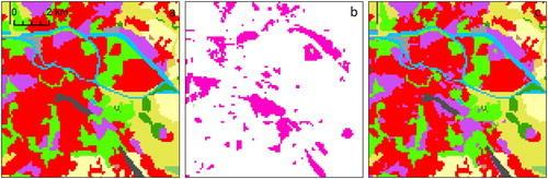
We further enhanced the result of previous operations by adding information from MultiNet® 3.6.2. by TomTom Global Content BV and TomTom North America, Inc. (formerly provided by TeleAtlas), an off-the-shelf proprietary vector database oriented primarily on routing and navigation (further referred to as TomTom). The database contains a polygon layer representing land use (such as industrial, commercial, public and transportation facilities as well as urban green areas; many of them smaller than 25 ha). The thematic detail is higher or equivalent to the CLC; hence an acceptable correspondence between the two schemes could be established. We included patches represented by one or more cells (Figure 5).

Figure 5. Including TomTom land use data in the map. A large majority of added polygons corresponded to the class ‘Industrial and commercial units’ (magenta patches in the box b). Legend for boxes a and c is provided in Figure 2(a).

3.1.4. European settlement map

The ESM intends to represent building cover fraction in the range 0%–100% (disregarding other impervious areas such as roads, city squares, railways, parking lots, and others). We augmented the Urban fabric class by areas extracted from ESM using a threshold (Figure 6). The Urban fabric (settlements) is the primary target in population distribution modelling. Hence, our objective was to capture also small hamlets, sparse settlements and even isolated houses/farms. To capture such settlements, we empirically derived a threshold yielding a trade-off between omission and commission errors at ESM value of 5%. We established this value based on a comparison of ESM with building density computed from reference building footprints in six sample regions (Portugal, Slovakia and United Kingdom). Apart from introducing new urban fabric areas, we used non built-up ESM cells (0%) to refine the shape of urban fabric patches present in the original CLC map. Urban fabric cells at the edges of patches scoring 0% as per the ESM data were converted to the closest non-artificial class in the vicinity.

Figure 6. Refining the urban fabric using European Settlement Map. The grey shade in box b. represents building density level (values above 5% were included). Legend for boxes a and c is provided in Figure 2(a).

3.1.5. Urban Atlas 2012

As of January 2017, UA data covered almost 600 urban areas in all EU and EFTA countries, covering 15% of the study area and ca 50% of its population (Figure 7), almost double compared to UA2006. The datasets portray urban LULC at 1 ha minimum mapping unit (0.25 ha for artificial surfaces) and 10 m minimum width, i.e. much finer than CLC (European Commission 2016). Including this data significantly improves the spatial detail and accuracy of the affected areas (Figure 8); but at this point, we also introduce heterogeneity in the map – areas covered by UA data will have different level of detail and lineage than the remaining areas.

Figure 7. The study area (white) and the included larger urban zones covered by Urban Atlas data (dark grey).

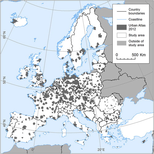
Figure 8. Refining the map using Urban Atlas data. Consult Figure 2(a) for legend.

The legend of UA2012 is analogous to that of CLC, but given the focus on urban areas, the thematic detail for non-artificial surfaces is reduced to the second or first level of CLC. On the other hand, the number of artificial classes is slightly higher. Out of the 27 classes of UA2012, 17 were assumed to have a direct semantic correspondence with CLC. For the remaining classes, we solved the disagreement by accepting the more detailed geometry of UA and deducing the missing thematic detail from the underlying data, based on proximity (Euclidean allocation).

The UA, as well as HRL, characterise waters and wetlands only at the first CLC thematic level. We used proximity to coastlines to discern Inland wetlands (41) from Marine wetlands (42), but further distinction of Inland wetlands into Inland marshes or Peat bogs was not feasible and the two classes are merged in the final map. Further, we analysed the shape of contiguous pixel groups in the HRL Permanent Water Bodies to identify rivers. The river layer was then used to separate and refine Water courses (511), although the shape-based distinction between river and lakes can become less clear in complex aquatic systems such as deltas.

3.1.6. Tomtom Multinet 2014 – built-up layer

Although ESM and UA data helped to detect many additional settlements, we looked for additional omissions. Municipalities in which the amount of urban fabric was zero or extremely low compared to expectation (given an empirical relationship between the sizes of the population and urban area) were enriched by adding built-up polygons from TomTom. This intervention was marginal, as it concerned only 1% of the 115 thousand municipalities in the study area.

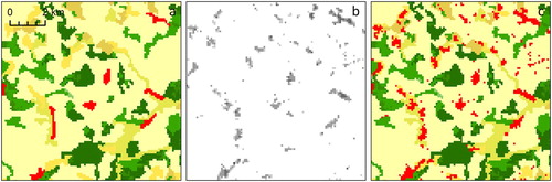
3.1.7. Linear features

Linear features such as rivers and road networks are important elements of the landscape due to their connecting and barrier effects. These effects are present even when the linear features are not dominant in terms of area. To ensure connectivity of the linear features, we updated the map by adding cells in which rivers or roads account for as little as 10% of the cell. Artificial areas were though replaced only when the fraction corresponding to the linear feature exceeded the ESM built-up density in the given cell. In this way, we included a river layer obtained from HRL Permanent water bodies and a road layer comprising motorways and main national roads from OSM and TomTom tunnel mask (Figure 9).

Figure 9. Refining the linear features of the map. Box b shows rasterised road layer derived from OSM data (grey) and a river mask extracted from HRL Permanent Water Bodies (light blue). Legend for boxes a and c is provided in Figure 2(a).

3.2. Thematic refinement

At this stage, we have obtained an intermediate result with refined spatial detail but thematically equivalent to original CLC. Below we describe the decomposition of 11 third-level classes of Artificial surfaces into 18 fourth-level classes (Table 1). The target scheme was affected by data availability, feasibility of continent-wide application, and foreseen applications of results.

3.2.1. Urban fabric

The representation of the Urban fabric resulting from the spatial refinement combined the Continuous and Discontinuous urban fabric (CLC classes 111 and 112) with settlements obtained from ESM and six UA classes of various density (11100, 11210, 11220, 11230, 11240 and 11300). To account for the variety of built-up densities, ranging from central business districts to scattered rural settlements, we defined four classes systematically, according to ESM building density (Figure 10):

• 1111 – Urban fabric high density (>50% built-up),

• 1121 – Urban fabric medium density (30%–50% built-up),

• 1122 – Urban fabric low density (10%–30% built-up),

• 1123 – Urban fabric very low density (<10% built-up) or isolated.

  Figure 10. Breaking down the ‘Urban fabric’ class based on ESM building density (the grey shades in the box b. correspond to the four selected density intervals). Legend for box a and c is provided in Figure 2(a and b), respectively.

  

To reduce noisy appearance of some urban areas, we sequentially filtered patches smaller than five cells. Contiguous groups of at least five high density urban cells formed class 1111. Smaller groups of high density cells were downgraded to medium density. Next, contiguous groups of minimum five medium density cells formed class 1121 while smaller groups were downgraded to low density. Finally, contiguous groups of at least five low density cells were considered as 1122, and the remaining cells (having less than 10% built-up or isolated groups of less than five cells regardless of built-up density) were classified as 1123.

3.2.2. Transportation

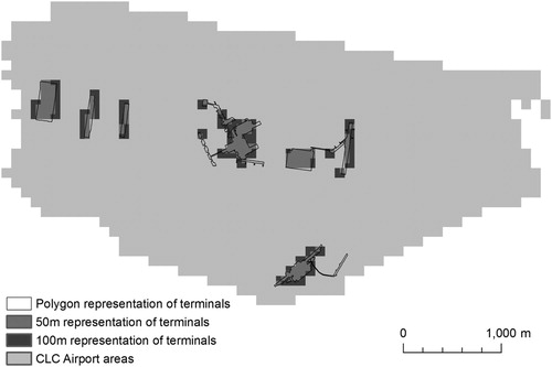
Knowing the locations of major transport terminals is significant for population modelling objectives. Such information has not been present in CLC maps, e.g. the representation of an airport area includes runways and surrounding grass land cover. We derived two additional classes 1242 (Airport terminals) and 1222 (Major stations) by incorporating polygon data from OSM. Since some of the polygons would disappear when rasterised directly at 100 m cell size, we exaggerated their representation using a two-step approach. First, we rasterised the polygons using 50 m cell size. Second, we aggregated the result to 100 m using the ‘maximum’ operator (Figure 11). The OSM-derived cells were allowed to replace only cells nested in the existing transportation classes so that potential error propagation from the crowdsourced data was constrained.

Figure 11. Conversion of terminal buildings polygons (OSM tag aeroway = terminal) into raster representation.

3.2.3. Sport and leisure facilities

According to the CLC technical guide (Bossard, Feranec, and Oťaheľ 2000), the class 142 Sport and leisure facilities contains both outdoor (green) facilities for sports, recreation and tourism as well as related buildings and infrastructure. However, for the population and employment distribution modelling the latter component is most significant. We decomposed the class into 1421 Sport and leisure green and 1422 Sport and leisure built-up by applying an ESM-based threshold of 10% building density.

3.2.4. Industrial and commercial units

To classify the ICU into predefined subclasses, we conducted a supervised machine learning classification. We describe the mains stages of the procedure: defining the individual observation units to be classified, labelling the training and test sets based on ancillary reference data, computing values of the predictor variables (features describing the spatial context based on POI data), and running the machine learning classification (using random forests algorithm). We provide a list of datasets introduced to facilitate the thematic refinement in Table 3.

Table 3. Specification of the data used in the thematic refinement, order by importance.

Ancillary land use data used to derive training labels (Section 3.2.4.2)
1	Map data 2017 copyrighted by OpenStreetMap contributors and available from https://www.openstreetmap.org
2	MultiNet® 3.6.2. © 2013 TomTom Global Content BV and TomTom North America, Inc.
3	SIOSE: Sistema de Información sobre Ocupación del Suelo de España, 2011.
	COS: Carta de Uso e Ocupação do Solo de Portugal, 2007.
	DUSAF 4.0: Uso del suolo Lombardia 2012.
	COSW: Carte d'occupation du sol de Wallonie version 2007
Point of interest data used to derive predictor variables (Section 3.2.4.2)
1	MultiNet® Points of Interest 1.9 © 2013 TomTom Global Content BV and TomTom North America, Inc.
2	Map data 2017, copyrighted by OpenStreetMap contributors and available from https://www.openstreetmap.org
3	EuroRegionalMap v9.1, EuroGeographics ©2014
4	Platts (2014). Platts is a source of data on energy, petrochemicals and metals, including geodata, provided by S&P Global.
5	E-PRTR, European Pollutant Release and Transfer Register, is a Europe-wide register of the main pollutan-t releasing industrial facilities.

The ICU class comprises non-residential land dedicated to various economic activities, and therefore it is particularly relevant for employment allocation. In fact, it comprises more activities than strictly industry and commerce, e.g. agricultural facilities, public services (such as schools and hospitals and government buildings), energy production, military areas and many other uses. Nevertheless, we assumed a broad scheme of relatively easily discernible subclasses that link to the following broad sectors according to the European statistical classification system of economic activities – NACE (Eurostat 2008):

• c₁ – 1211 Production facilities (NACE sectors A, B, C, D, and E),

• c₂ – 1212 Commercial/service facilities (NACE sectors G, H, I, J, K, L, M, and N),

• c₃ – 1213 Public facilities (NACE sectors O, P, and Q).

A more detailed breakdown would likely complicate the classification, for example, various subsectors of services can be spatially intertwined at the level of the individual cells, or even buildings. Besides, some narrow sectors might be too rare to yield a sufficient number of training examples.

3.2.4.1. Defining observation units

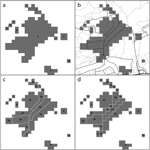
Each target entity had to be characterised by a series of predictor variables (features) derived by relatively demanding geo-computation (described in the next section). Two types of entities could be readily obtained from the raster map – individual cells or contiguous clusters of cells. While the former were too numerous, increasing computational cost significantly (over 4 million); the latter often spanned large interconnected portions of cities, lacking necessary spatial detail. Therefore we opted for contiguous clusters segmented by TomTom roads layer that included categories ranging from motorways to local roads (i.e. TomTom road categories 0–6) and excluded local roads of minor importance and others (i.e. 7–8). Resulting segments too small/narrow to be represented by 100 m cells were merged with an adjacent polygon based on edge length (Figure 12). In the end, we obtained ca 740 thousand polygons; further referred to as the target polygons.

Figure 12. Geometrical segmentation of the industrial and commercial clusters by the road network (a. vectorised clusters as per the spatial refinement, each with a unique identifier; b. road network used to segment the polygons; c. segmented polygons after elimination of sliver segments; and d. segmented polygons after rasterisation).

3.2.4.2. Deriving reference labels for training and testing

To train the classifier, we labelled a subset of the target polygons based on intersection with at least one of three ancillary land use datasets:

• d₁ – selected polygons from OSM (mostly selected by landuse and building keys)

• d₂ – land use polygons from TomTom

• d₃ – a compilation of polygons from four national/regional land use datasets with suitable classification system (see Table 3 for details)

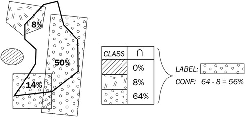
The notion of economic activity in the ancillary data attributes/annotation allowed us to create a semantic link with target class c_i and calculate the relative area of intersection between each target polygon and class c_i in ancillary dataset $d_j\left({\cap }_{c_i{d}_j}\right)$. Further, we defined a confidence score $CON{F}_{c_i}$ of a target polygon belonging to class c_i that increases with the total area of c_i intersections and decreases with the total area of the other classes’ intersections (Equation (1), Figure 13).(1) $CON{F}_{c_1}=\sum _{j=1}^3{\cap }_{c_1{d}_j}-\sum _{j=1}^3{\cap }_{c_2{d}_j}-\sum _{j=1}^3{\cap }_{c_3{d}_j}$(1) The class with the highest $CON{F}_{c_i}$ was set as the label per each target polygon. While the maximum of 300% was possible (d₁, d₂ and d₃ indicating full intersection by the same class), we fixed the minimum requirement as 30% $CON{F}_{c_i}$ and at least one ${\cap }_{c_i{d}_j}$ of 30% or more. The 30% threshold presents a more relaxed condition than the typical dominance criterion of 50%, compensating imperfect overlaps due to rasterised shapes of polygons (Figure 11(a)) and positional inaccuracies. As a result, around 270,000 target polygons were labelled (about 36% of the total number to be classified). Assignment of the label confidence values allowed for later tuning of the training set size and reliability.

Figure 13. An illustration of obtaining a training label and its confidence score, based on cumulative relative intersection area per class, across ancillary land use datasets.

3.2.4.3. Deriving predictor variables (features)

We compiled a database of POI data related to economic activities (over 12 million points) from TomTom, OSM, EuroRegionalMap (from EuroGeoraphics), E-PRTR and PLATTS (for details consult Marin Herrera et al. 2015, 28). Then we characterised the target polygons by the frequency of POI in the polygon interior by category (DIPOI variables). To account for positional inaccuracies, and to sense geographical context of polygons containing no POI, the nearby POI were considered too, weighted by a distance decay function (WSPOI variables, Equation (2)). We assumed POI of category c present in the target polygon neighbourhood increase the probability of polygon affiliation with the class c, and that the amount of increase is inversely proportional to the POI distance from the polygon (Figure 14).(2) $WSPO{I}_c=\sum _{pϵc}{\left(1-\frac{DISTANC{E}_p}{CUTOFF}\right)}^{DECAY}$(2) We considered a wide search distance (CUTOFF = 700 m) with a steep decay function (DECAY = 5), so that the more distant POI have lesser importance compared to the contained ones, but still have some effect if there are no closer POI. In total, six POI-derived variables were the primary features fed to the machine learning classification. Despite the comprehensive POI database, 17% of the target polygons (10% of the ICU area) did not have any POI in their interior or within the cut-off. Therefore we enriched the dataset by adding contextual variables based on other available geodata (listed in Table 4).

Figure 14. An illustration of deriving the DIPOI and WSPOI predictor variables based on the POI locations inside and around a polygon.

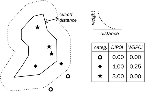
Table 4. List of predictor variables included in the final model.

DIPOI_c	Number of class c POI directly intersecting the polygon (three variables)
WSPOI_c	The weighted sum of class c POI within the cut-off distance from the polygon (three variables)
AvgESM	The average ESM-based building density within the polygon
LogDist_f	Log distance to feature category f ∈ [highway, railway, port, airport, city centre]
LogPopDens	Log Population density within 500 m buffer around the polygon
LCshare_k	The share of land cover class k ∈ [artificial, agricultural, natural, wetland and water] in a 500 m buffer area
Area	Surface area of the polygon
AdjRefVal	The reference label of the neighbouring polygon with the longest shared edge (if present)

3.2.4.4. Machine learning classification

We used random forest classification (Breiman 2001a), to predict land use classes using the derived predictor variables. This method has been successfully used in complex scenarios, such as classification of multitemporal/multispectral remote sensing datacubes (Mack et al. 2017; Schultz et al. 2017), disaggregation of census data (Stevens et al. 2015), and other tasks with large number of observations. The algorithm averages multiple decision trees built on a data set. Each tree is constructed from different subsets from the training dataset, created by bootstrapping (random resampling with replacement) leaving aside the so-called ‘out of bag’ data. At each node of the tree a subset of the total number of predictor variables are selected at random, and the variable that reduces most node impurity is used to do a binary split on that node. Each tree gives a classification validated on ‘out of bag’ data and final prediction is the averaged value of all the trees. The supervised random forests can ingest a large number of variables, including categorical ones, can avoid overfitting by bootstrap aggregating, and provides a probability of each class per individual observations. Moreover, it can derive feature importance from the data (Breiman 2001b) and deal with correlated features, so that the pre-classification data selection can be less rigorous (Schultz et al. 2017, 208).

Due to computational constraints, we did not optimise the hyperparameters systematically, but we manually explored various settings. We investigated several specifications of the training set (controlled by various confidence thresholds), and different configurations of the predictor variables (e.g. including/excluding variables, log-transformation of distance and population variables, and merging DIPOI and WSPOI variables). In total, we ran 50 models using H₂O, a machine learning library for R that can handle big datasets. One thousand trees (ntree) was the number beyond which there was no significant increase in performance. We kept the default choice of the number of variables (mtry), i.e. 1/3 of the total feature count. The best performing model used a training set with a confidence level above 50 (ca 225,000 polygons) out of which 30% was left aside for testing and 70% for actual model training.

3.2.4.5. Deriving an independent validation sample

We selected a random sample of 600 target polygons, for which the ground truth label was blindly interpreted (without knowing the predicted values), relying on the time series of aerial images in Google Earth, to see whether the area remained stable or undergone changes. We investigated street-view photos too, where available. The image dated closest to 2012 was crucial for the final decision. We defined the ground truth label as the dominant ICU subclass inside the bounds of the polygon, preferring the aspect of economic sector over the built-up morphology. For example, if wholesale, storage and distribution firms prevailed in an industrially-looking zone, we considered it as class 1212 (Commercial/service facilities).

4. Results

4.1. Performance of the random forest classification

The selected random forests model for classification of ICU yielded an overall accuracy of 87% when compared with the 30% of training set reserved for validation (Table 5). The Cohen’s Kappa coefficient of 0.72 indicates substantial agreement (Landis and Koch 1977). The notion of land use present in the ancillary data was transferred to the target polygons successfully. The most abundant class, ‘Production facilities’, was predicted with the least error (11.1% commission and 4.6% omission error). Greater commission (18.5% and 14.9%) and omission (36.1% and 23.5%) errors were recorded for the remaining classes. While the accuracy was within acceptable range for ‘Public facilities’, the accuracy of ‘Commercial/service facilities’ prediction was hindered by frequent confusion with ‘Production facilities’.

Table 5. Confusion matrix of the selected random forest model classification result.

Overall accuracy: 87.4% Cohen’s Kappa: 0.72		Prediction
		1211	1212	1213	Total reference	Omission error
Reference	1211	44,106	1,262	870	46,238	4.6%
	1212	3,298	6,831	558	10,687	36.1%
	1213	2,229	285	8,166	10,680	23.5%
	Total predicted	49,633	8,378	9,594	67,605
	Commission error	11.1%	18.5%	14.9%

4.2. Independent validation results

Despite the prior segmentation by roads, a significant share of the interpreted polygons appeared mixed. Production and commercial/service facilities frequently co-occurred, partly due to the gradual transformation of former industrial zones to ‘softer’, commerce-related activities (storage, transport, wholesale and retail). In such cases, we identified the prevailing subclass, except for the 9% of polygons where two (or three) classes were mixed equally, or street-level imagery was not available. Another 13% of polygons were commission errors of the ICU per se (in reality being, for instance, residential or non-built up areas). These were either inherited from the source information on ICU (CLC, UA and TomTom) or caused by geometric inaccuracy; less frequently a temporal mismatch might have contributed as well.

First, we report validation of the training labels obtained from the ancillary LULC data, as they have errors of their own. The land use classification in the ancillary datasets is semantically loose, partially mapped by volunteers without in-situ knowledge by digitisation on top of aerial imagery. The overall accuracy of the training data was lower than expected (78.5%, 0.64 Kappa, Table 6), when confronted with the narrow definition of economic sectors. The most prevalent error is indeed the confusion between Production and Commercial/service facilities. On the other hand, the Public facilities are captured with good accuracy, perhaps thanks to less ambiguous semantics.

Table 6. Validation of the reference labels against the visually interpreted ground truth.

Overall accuracy: 78.5% Cohen’s Kappa: 0.64		Prediction
		1211	1212	1213	Total reference	Omission error
Reference	1211	112	14	5	131	14.5%
	1212	29	35	0	64	45.3%
	1213	3	4	54	61	11.5%
	Total predicted	144	53	59	256
	Commission error	22.2%	34.0%	8.5%

Consequently, the errors of reference labels against the ground truth (Table 6) cumulated with the prediction errors (Table 5) and lowered the accuracy of the predicted labels compared to ground truth to 72.1% (0.48 Kappa). However, the predicted class (one with the highest probability) was not included in the final map for:

• Cases with an assigned label (36% of the target polygons) – the label was used instead of prediction

• Cases in which the highest class probability was less than double compared to the second highest one, and there was a label assigned to an adjacent target polygon (AdjRefVal was used instead of prediction).

The overall accuracy of the ICU classification eventually represented in the final map was 74% (Kappa 0.53), as shown in Table 7.

Table 7. Validation of the final values included in the map against the visually interpreted ground truth.

Overall accuracy: 74.0% Cohen’s Kappa: 0.53		Prediction
		1211	1212	1213	Total reference	Omission error
Reference	1211	232	16	9	257	9.7%
	1212	73	40	5	118	66.6%
	1213	13	5	73	91	19.8%
	Total predicted	318	61	87	466
	Commission error	27.0%	34.4%	16.1%

4.3. Comparison of CLC2012 and resulting refined map

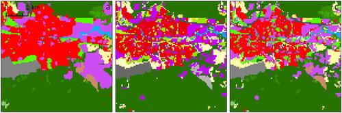
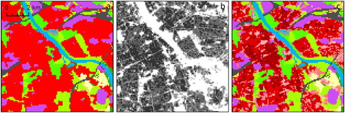
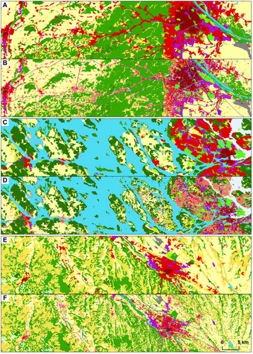
Figure 15 compares the original and refined maps in full thematic resolution. The selected areas comprise various settlement types from metropolitan to dispersed rural ones. The highest level of refinement is evident in the urban area – the LULC texture of cities is, in reality, more fine-grained compared to an exurban setting, and this detail is well captured in the urban area covered by UA data. Roughly the west half of each transect is though located outside of urban area; here only the artificial classes, forest, wetlands and water are refined (at the inferior spatial detail of 5 ha). Nevertheless, the dichotomy is not markedly visible, which is an important aspect of the map’s cartographic quality.

Figure 15. Comparison of original CLC (A, C, D) and the final refined result (B, D, E). A and B show Vienna and its westward hinterland, C and D show Stockholm with its hinterland, E and F show rural landscape around the town of Pau (southwest France). See Figure 2 for legends.

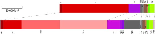
The increased spatial detail altered the abundance of individual classes. Table 8 shows the transitions between classes and total class area change, aggregated to the second level of CLC legend for simplicity. Frequently, newly added Urban fabric (11) replaced the surrounding Arable land (21) and other crops (22, 23). Overall, the Urban fabric area grew by over 50%, despite some loss to Arable land and Pastures (shape of some urban fabric patches was ‘de-generalised’ by removing the non-built fringe). Around 6% of original Urban fabric changed to Industrial, commercial and transport units (12) by introducing the TomTom and UA data and the road networks. Due to the road network exaggeration and additional patches of ICU the area of class 12 more than doubled. Significantly modified were Artificial non-agricultural vegetated areas (14). These are abundant mostly in urban areas (parks and green spaces), which were reconfigured by UA data. Part of the class was reclassified to Forest and Pastures (minor interpretation differences between UA and CLC might have played a role), but its overall area increased as new small patches (<25 ha) replaced Urban fabric in many cities.

Table 8. Class transitions due to spatial refinement aggregated to CLC level 2 for clarity (all percentages are relative to CLC2012; the green-red colour scale represents the degree of modification of the origin class from the highest to the lowest; the grey represents the proportion of the origin class reclassified to the respective result class).

In relative terms, the non-artificial classes were less affected compared to the artificial ones, except for the Heterogeneous agricultural areas (24). Unsurprisingly, these diminished the most due to their mosaicked LULC pattern. They often include scattered settlements not captured as UF by CLC, but detected by ESM. In areas covered by UA data, the mosaic was also partly decomposed to patches of Arable land, Pastures and Forests (31). Forests expanded overall by 6% as the HRL Tree cover density discriminated further small patches from the Heterogeneous agricultural areas (24) as well as Shrub/herbaceous (32) and Pastures (23). The decrease of Shrub/herbaceous areas mostly relates to the subclass of Transitional woodland shrub (324) that is prone to be interpreted as forest by the HRL Tree cover density. The HRL Permanent water bodies and exaggeration of rivers expanded the Inland waters by 9%.

We further illustrate the changed abundance and breakdown of Artificial surfaces to the fourth level in Figure 16. The surface area expanded or remained stable for most of the third-level classes. The ICU expanded by 45% while Road/rail networks and associated land expanded substantially (over tenfold). Green urban areas almost doubled and Sport and leisure facilities expanded by 27%. At the fourth level, the Urban fabric had a heavy-tailed distribution with very small area of the dense and the largest area of the very low density class. 75% of the ICU area was classified as Production facilities, 13% as Commercial/service facilities and 12% as Public facilities. This distribution corresponds to the class proportions of the training sample (74%, 14% and 12% respectively). The newly created transportation terminal classes (1222 and 1242) occur only in the order of thousands of hectares (not displayed in Figure 16). Around 30% of Sport and leisure facilities area was classified as Sport and leisure built-up.

Figure 16. Areas of original and refined classes of artificial surfaces. Consult Table 1 for class code-label correspondence.

5. Discussion

Previously, the state-of-the art Europe-wide data on LULC referring to the year 2012 was either insufficiently detailed (CLC), patchy in coverage (UA), or thematically restricted (ESM, HRL, TomTom). We combined these and datasets with additional POI and polygon data into a single, readily usable map that maximises the portrayed spatial and thematic detail. The resulting continental-scale layer has a spatial detail of one hectare, except for non-artificial classes outside of urban areas (Figure 6), which are mapped at five hectares. Furthermore, we expanded the nomenclature of artificial classes from 11 to 18 classes, using additional spatial data. The result presents a new valuable asset with a high potential to underpin diverse research in topics and at scales that are relevant for policy makers. Although the reference year may seem outdated, it reflects the availability of its constituent datasets (for instance, Urban Atlas 2012 data for some European cities were still under production as of 2018). The reference year is also, conveniently, close to the most recent (2011) census data that are often used along LULC maps.

From the methodological perspective, we were able to adapt the spatial refinement approach of Batista e Silva, Lavalle, and Koomen (2013) for the currently available data – partly thanks to the continuity of EU’s Copernicus land-monitoring services. The thematic refinement of selected artificial classes was achieved either by a cartographic overlay approach (for Urban fabric, Sport and leisure facilities, Airports and Road, rail and associated land) or by machine learning classification (Industrial and commercial units). The latter presents a novel experimental method, supported by a comprehensive data on economic activities in POI form (for predictor variables) and ancillary land use polygons (for model training and testing).

Compiling sufficiently complete database of POI data required more relaxed criteria on temporal consistency. While in the spatial refinement phase all the data related to 2012 ± 1 year (Table 2), the thematic refinement could be guided in some cases by information obtained or recorded as late as 2017 (Table 3). This mismatch might have contributed to the error of machine learning classification; however it could not influence the spatial domain of the map that was defined in the spatial refinement stage. Therefore we assumed the merit of using the respective data outweighed the potentially induced errors.

The employed machine learning approach allowed us to classify, across Europe, 740 thousand polygons of a very heterogeneous land use class into a breakdown of three more specific classes linked to economic classification, using available data, in a fairly expedite, accurate and low cost manner. The best random forests classifier achieved over 87% accuracy (Kappa 0.72) – this represents the model fitness vis-à-vis the testing set, labelled based on proprietary, volunteered, and public land use data (the same labelling approach as used for training). Nevertheless, the data used to derive the reference labels proved to be noisier than expected (78.5% accuracy, 0.64 Kappa), when compared to more strictly defined ground truth (the dominant sector-based land use). Consequently, the accuracy of the ICU classification in the final map was 74% (Kappa 0.53) with a high omission rate of Commercial/service facilities (classified instead as Production facilities). We attribute the high confusion of this specific class pair to two deeper factors:

• Semantic ambiguity of the term ‘industrial’ – the discrepancy between the morphological and functional (sectoral) notions of it;

• Actual co-occurrence of production facilities and a branch of commerce and services including storage, distribution, logistics and wholesale. This pattern is further amplified by deindustrialisation and conversion of former industrial buildings to retail/offices, such that an apparently industrial zone of a city might become predominantly commercial.

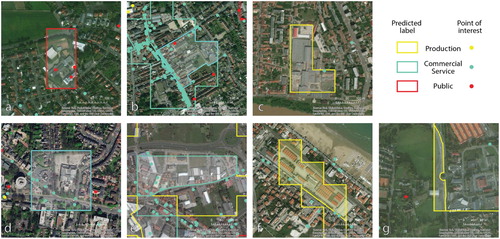
In Figure 17 we provide detailed examples of polygons and their predicted label. The upper row (Figure 17(a–c)) represents correctly classified polygons. Note that the commercial/service POI tend to occur in more numerous clusters unlike the other two categories. In Figure 17(c) it is evident that the classifier correctly learned that a commercial/service area is typically manifested by such a clustering – a single POI was not sufficient clue. On the contrary, the production facilities were likely identified by absence of a larger number of commercial/service POI or a public POI. Figure 17(d and e) show dominantly public and production polygons respectively, confused as commercial/service due to occurrence of the POI cluster. In both cases, the POI are concentrated in one part of the polygon, thus we can assume these polygons are in fact mixed. The classification would likely be more successful if the polygons were more finely segmented. The polygon in Figure 17(f) is misclassified as production facility due to lack of suitable contextual information (in reality, the object is a police facility, i.e. a public service). The last example (Figure 17(g)) represents a commission error in the set of target polygons. As a result of the segmentation, some of smaller ICU polygons might actually be non-built up areas. Hence, assignment of any of the three labels would be wrong.

Figure 17. Examples of correctly predicted labels (a–c), incorrectly predicted labels (d–f), and a problematic case (g).

This illustrates the difficulty of the performed task – inherent errors from input datasets, semantic discrepancies and noise emerging from combining several imperfect sources as well as the fuzzy nature of the studie phenomena hindered the inference at most stages of the work. Therefore, the ICU classification should not be considered as sharply categorical, but rather probabilistic.

Based on visual examination of the results, we acknowledge further complexities and limitations pertaining to the spatial refinement phase. We combined the input datasets without manual interventions, based on decision rules assuming that each dataset correctly represents the respective theme. In reality, classification errors are inevitable in continental-scale datasets (semi-)automatically derived from satellite imagery, and these propagate into the final product. In case of the ESM, other objects than buildings could have been mapped, such as bare rocks or soil, vehicles and transport infrastructure. The forests derived from HRL tended to replace olive groves, orchards and agroforestry in some areas. Hence we restricted such class transitions by specific rules. We also speculate that the HRL might have captured spectrally and semantically distinctive water surfaces more accurately than wetlands, which might have been confused with agriculturally used wet soils or with areas classifiable as forests.

Other errors might have ensued from the applied decision rules. Extracting urban fabric from the ESM required a threshold to discretise the interval ESM values. The goal to detect isolated settlements was achieved by selecting values above 5%, which minimised the sum of commission and omission errors when evaluated in selected test-sites (Portugal, Slovakia and the United Kingdom). However, there might be no single universal optimum, and the distribution of ESM values may be variously biased across ecoregions due to land cover colour and pattern characteristics of the landscape (Pesaresi et al. 2013, 2125). For instance, the arid interior of Iberian Peninsula might have positively offset ESM values due to sparse vegetation (leading to prevalent commission errors at the given threshold); while the opposite might be true in some other regions.

Including the TomTom and UA data relied on semantic correspondence between polygon categories and target LULC classes. The linkages were not always perfect, which may have caused errors compared to the target definitions (for example, greenhouses are recorded in UA as ICU, while according to CLC they belong to agriculture). Moreover, in case of non-agricultural classes of UA, the correspondence was possible only at second or even first level of CLC. The class at the third level was then established based on the nearest from the suitable subset of classes (Euclidean allocation method). Such solution is satisfactory provided that there is a good agreement between CLC and UA at the second level of LULC classification. Otherwise, spurious results might occasionally arise, although confusion would occur only between semantically similar classes.

Introducing the TomTom and UA data increased the average levels of spatial detail and map refinement significantly, but also reduced the spatial consistency and homogeneity as TomTom completeness varies across countries and UA covers only larger urban areas. To better refine areas without good coverage of UA/TomTom, OSM polygon data might be leveraged. Several studies suggest that despite being collected by volunteers, the OSM data has a great value and should not be overlooked (Dorn, Törnros, and Zipf 2015; Jokar Arsanjani and Vaz 2015) and attempts were made to produce LULC maps from OSM (Jokar Arsanjani et al. 2013; Estima and Painho 2015; Fonte et al. 2017; Schultz et al. 2017). Our experience was similar – the data proved to be valuable for labelling of the training data and the mapping of transport terminals. The OSM geometries often seem to be as complete and detailed as proprietary or public authority data. Although the completeness may vary from region to region, it has been increasing over time. The drawback is that annotation may be insufficient, incorrect or difficult to extract due to the free-from tag scheme (Fan et al. 2014); incorrect tags can cause infrequent but great-magnitude errors.

As a suggestion for future research, we think that a more detailed classification of economic activities would be useful for addressing several policy relevant topics. Given the limitations of the presented approach, we propose two avenues. The first avenue would continue in the attempt to exhaustively classify the land, even when the activities are mixed (i.e. the dominant prevails). This would ideally require finer target units (individual cells or polygons segmented using all intersecting roads and railways), but some degree of class mix is inevitable (even single building can sometimes host multiple sectors). Using high-performance computing might facilitate advancement of the spatial resolution (e.g. to 50 m), which would reduce ambiguity and harvest more information from detailed input datasets (UA and potentially OSM polygons). The other avenue would be to acknowledge the intrinsic mix-up of some economic activities by allowing for a Sector mix class or by assessing the share of each sector in the polygon, instead of a categorical classification. In such case, an alternative data model would need to be considered. It is not practical to attach multiple attributes to the target entities via a single raster dataset.

6. Conclusion

Europe-wide data on land use/land cover for the year 2012 have been either insufficiently detailed (CLC), patchy in coverage (UA, TomTom), or thematically restricted (ESM, HRL). We describe a method of combining these and other datasets into a single readily usable map that combines the best of the source datasets. Apart from the spatial refinement (from 25 ha to 1 ha) we expanded the number of thematic classes to 50. The novel contribution involved a machine learning classification of industrial and commercial polygons into three subclasses (Production facilities, Commercial/service facilities and Public facilities). After segmenting the polygons by road network, we labelled a training subset of the segments based on intersection with ancillary data, where available. Consequently, we characterised the full set by features derived from spatial analyses performed on a large volume of geodata (several categories of POI, transport infrastructure, population and building density). Finally, we ran multiple instances of random forests classification algorithms and evaluated the selected model using and independent validation.

The machine learning classification performed at 87% overall fitness successfully replicating the notion of activities present in the training data. However, the training data were noisier than expected, leading to lower accuracy levels (74%) measured by the independent validation. Nevertheless, the significance of the results is demonstrated by two on-going applications at the European Commission's Joint Research Centre. In the context of ENACT project (‘ENhancing ACTivity and population mapping’, Batista e Silva et al. 2017) an effort is underway to produce EU-wide daytime and night-time population grids per each month of a year. The resulting 100 m raster map will serve as the main covariate in the population modelling, along with a stack of binary layers mapping further specific activities/population subgroups. The refined map is to be employed by the LUISA Territorial Modelling Platform that projects land use changes and population distribution at 100 m resolution until 2050 (Lavalle et al. 2016; Jacobs-Crisioni et al. 2017). The results are envisaged to be useful in other applications, such as creating more accurate models of air pollution distribution.

Disclaimer

The views expressed are purely those of the authors and may not in any circumstances be regarded as stating an official position of the European Commission.

Acknowledgements

This study was done in the context of the ENACT project (ENhancing ACTivity and population mapping) of the European Commission Joint Research Centre, with the following project team: Filipe Batista e Silva, Konštantín Rosina, Mario Marín, Carlo Lavalle, Marcello Schiavina, Sérgio Freire, Thomas Kemper, Lukasz Ziemba and Massimo Craglia. The authors would like to thank Carlo Lavalle for his continuous support, and the reviewers for their useful comments and suggestions.

Data availability

The resulting map can be accessed in GeoTIFF format. DOI:10.6084/m9.figshare.6210392.

Disclosure statement

No potential conflict of interest was reported by the authors.

ORCID

Konštantín Rosina http://orcid.org/0000-0002-4696-1320

Filipe Batista e Silva http://orcid.org/0000-0002-8752-6464

Pilar Vizcaino http://orcid.org/0000-0002-7508-1568

Mario Marín Herrera http://orcid.org/0000-0003-4177-9471

Sérgio Freire http://orcid.org/0000-0003-2282-701X

Marcello Schiavina http://orcid.org/0000-0003-3399-3400

References

- Antoniou, V., C. Fonte, L. See, J. Estima, J. Arsanjani, F. Lupia, and S. Fritz. 2016. “Investigating the Feasibility of Geo-Tagged Photographs as Sources of Land Cover Input Data.” ISPRS International Journal of Geo-Information 5 (5): 64. doi: 10.3390/ijgi5050064
- Aubrecht, C., D. Özceylan Aubrecht, J. Ungar, S. Freire, and K. Steinnocher. 2017. “VGDI - Advancing the Concept: Volunteered Geo-Dynamic Information and its Benefits for Population Dynamics Modeling.” Transactions in GIS 21 (2): 253–276. doi: 10.1111/tgis.12203
- Batista e Silva, F., C. Lavalle, and E. Koomen. 2013. “A Procedure to Obtain a Refined European Land Use/Cover Map.” Journal of Land Use Science 8 (3): 255–283. doi: 10.1080/1747423X.2012.667450
- Batista e Silva, F., K. Rosina, M. Schiavina, M. Marin, S. Freire, M. Craglia, and C. Lavalle. 2017. “Spatiotemporal Mapping of Population in Europe: The ‘ENACT’ Project in a Nutshell.” Proceedings of the 57th European Regional Science Association (ERSA) Congress, Groningen, The Netherlands, 17 p.
- Ben-Asher, Z., H. Gilbert, H. Haubould, G. Smith, and G. Strand. 2013. HELM-Harmonised European Land Monitoring: Findings and Recommendations of the HELM Project. Tel-Aviv: The HELM Project.
- Bossard, M., J. Feranec, and J. Oťaheľ. 2000. CORINE Land Cover Technical Guide – Addendum 2000. Technical Report 40. Copenhagen: European Environment Agency. http://www.eea.europa.eu/publications/tech40add.
- Breiman, L. 2001a. “Random Forests.” Machine Learning 45 (1): 5–32. doi: 10.1023/A:1010933404324
- Breiman, L. 2001b. “Statistical Modeling: The Two Cultures (with Comments and a Rejoinder by the Author).” Statistical Science 16 (3): 199–231. doi: 10.1214/ss/1009213726
- Büttner, G. 2014. “CORINE Land Cover and Land Cover Change Products.” In Land Use and Land Cover Mapping in Europe, edited by I. Manakos and M. Braun, 55–74. Dordrecht: Springer.
- Cruickshank, M. M., R. W. Tomlinson, and S. Trew. 2000. “Application of CORINE Land-Cover Mapping to Estimate Carbon Stored in the Vegetation of Ireland.” Journal of Environmental Management 58 (4): 269–287. doi: 10.1006/jema.2000.0330
- Diaz-Pacheco, J., and J. Gutiérrez. 2014. “Exploring the Limitations of CORINE Land Cover for Monitoring Urban Land-Use Dynamics in Metropolitan Areas.” Journal of Land Use Science 9 (3): 243–259. doi: 10.1080/1747423X.2012.761736
- Dorn, H., T. Törnros, and A. Zipf. 2015. “Quality Evaluation of VGI Using Authoritative Data—A Comparison with Land Use Data in Southern Germany.” ISPRS International Journal of Geo-Information 4 (3): 1657–1671. doi: 10.3390/ijgi4031657
- EEA (European Environment Agency). 2007. “CLC2006 Technical Guidelines.” EEA Technical Report No 17/2007. 66 p. ISSN 1725–2237.
- Estima, J., and A. Painho. 2015. “Investigating the Potential of OpenStreetMap for Land Use/Land Cover Production: A Case Study for Continental Portugal.” In OpenStreetMap in GIScience, edited by J. Jokar Arsanjani, A. Zipf, P. Mooney, and M. Helbich, 273–293. Cham: Springer International Publishing.
- European Commission. 2011. “Mapping Guide for a European Urban Atlas [2006].” 30 p. https://www.eea.europa.eu/data-and-maps/data/urban-atlas/mapping-guide/urban_atlas_2006_mapping_guide_v2_final.pdf.
- European Commission. 2016. “Mapping Guide for a European Urban Atlas v4.7 [2012].” 39 p. http://land.copernicus.eu/user-corner/technical-library/urban-atlas-2012-mapping-guide-new.
- Eurostat. 2008. NACE Rev. 2 – Statistical Classification of Economic Activities in the European Community. Luxemburg: Office for Official Publications of the European Communities.
- Fan, H., A. Zipf, Q. Fu, and P. Neis. 2014. “Quality Assessment for Building Footprints Data on OpenStreetMap.” International Journal of Geographical Information Science 28 (4): 700–719. doi: 10.1080/13658816.2013.867495
- Feick, R., and C. Robertson. 2015. “A Multi-Scale Approach to Exploring Urban Places in Geotagged Photographs.” Computers, Environment and Urban Systems 53: 96–109. doi: 10.1016/j.compenvurbsys.2013.11.006
- Ferri, S., V. Syrris, A. Florczyk, M. Scavazzon, M. Halkia, and M. Pesaresi. 2014. “A New Map of the European Settlements by Automatic Classification of 2.5 m Resolution SPOT Data.” 2014 IEEE Geoscience and Remote Sensing Symposium, 1160–1163.
- Fisher, P., A. Comber, and R. Wadsworth. 2005. “Land Use and Land Cover: Contradiction or Complement.” In Re-Presenting GIS, edited by D. J. U. Peter Fisher, 85–98. Chichester: John Wiley and Sons.
- Fonte, C., M. Minghini, J. Patriarca, V. Antoniou, L. See, and A. Skopeliti. 2017. “Generating Up-to-Date and Deled Land Use and Land Cover Maps Using OpenStreetMap and GlobeLand30.” ISPRS International Journal of Geo-Information 6 (4): 125. doi: 10.3390/ijgi6040125
- Frias-Martinez, V., and E. Frias-Martinez. 2014. “Spectral Clustering for Sensing Urban Land use Using Twitter Activity.” Engineering Applications of Artificial Intelligence 35: 237–245. doi: 10.1016/j.engappai.2014.06.019
- Gallego, F., F. Batista, C. Rocha, and S. Mubareka. 2011. “Disaggregating Population Density of the European Union with CORINE Land Cover.” International Journal of Geographical Information Science 25 (12): 37–41. doi: 10.1080/13658816.2011.583653
- Jacobs-Crisioni, C., V. Diogo, C. Perpiña Castillo, C. Baranzelli, F. Batista e Silva, K. Rosina, B. Kavalov, and C. Lavalle. 2017. The LUISA Territorial Reference Scenario 2017: A Technical Description. Luxembourg: Publications Office of the European Union. ISBN 978-92-79-73866-1.
- Jacobs-Crisioni, C., P. Rietveld, E. Koomen, and E. Tranos. 2014. “Evaluating the Impact of Land-Use Density and Mix on Spatiotemporal Urban Activity Patterns: An Exploratory Study Using Mobile Phone Data.” Environment and Planning A 46 (11): 2769–2785. doi: 10.1068/a130309p
- Janssen, S., G. Dumont, F. Fierens, and C. Mensink. 2008. “Spatial Interpolation of air Pollution Measurements Using CORINE Land Cover Data.” Atmospheric Environment 42 (20): 4884–4903. doi: 10.1016/j.atmosenv.2008.02.043
- Jiang, S., A. Alves, F. Rodrigues, J. Ferreira, and F. C. Pereira. 2015. “Mining Point-of-Interest Data from Social Networks for Urban Land Use Classification and Disaggregation.” Computers, Environment and Urban Systems 53: 36–46. doi: 10.1016/j.compenvurbsys.2014.12.001
- Jokar Arsanjani, J., M. Helbich, M. Bakillah, J. Hagenauer, and A. Zipf. 2013. “Toward Mapping Land-use Patterns from Volunteered Geographic Information.” International Journal of Geographical Information Science 27 (12): 2264–2278. doi: 10.1080/13658816.2013.800871
- Jokar Arsanjani, J., L. See, and A. Tayyebi. 2016. “Assessing the Suitability of GlobeLand30 for Mapping Land Cover in Germany.” International Journal of Digital Earth 9 (9): 873–891. doi: 10.1080/17538947.2016.1151956
- Jokar Arsanjani, J., and E. Vaz. 2015. “An Assessment of a Collaborative Mapping Approach for Exploring Land Use Patterns for Several European Metropolises.” International Journal of Applied Earth Observation and Geoinformation 35: 329–337. doi: 10.1016/j.jag.2014.09.009
- Kunze, C., and R. Hecht. 2015. “Semantic Enrichment of Building Data with Volunteered Geographic Information to Improve Mappings of Dwelling Units and Population.” Computers, Environment and Urban Systems 53: 4–18. doi: 10.1016/j.compenvurbsys.2015.04.002
- Landis, J. R., and G. G. Koch. 1977. “The Measurement of Observer Agreement for Categorical Data.” Biometrics 33 (1): 159–174. doi: 10.2307/2529310
- Langanke, T., G. Büttner, H. Dufourmont, D. Iasillo, M. Probeck, M. Rosengren, A. Sousa, P. Strobl, and J. Weichselbaum. 2016. GIO Land (GMES/Copernicus Initial Operations Land) High Resolution Layers (HRLs) – Summary of Product Specifications, Version 13. EEA Copenhagen.
- Lavalle, C., F. Batista e Silva, C. Baranzelli, C. Jacobs-Crisioni, I. Vandecasteele, A. L. Barbosa, and S. Vallecillo. 2016. “Land Use and Scenario Modeling for Integrated Sustainability Assessment.” In European Landscape Dynamics, edited by J. Feranec, T. Soukup, G. Hazeu, and G. Jaffrain, 237–262. Boca Raton, FL: CRC Press.
- Liu, Y., X. Liu, S. Gao, L. Gong, C. Kang, Y. Zhi, and L. Shi. 2015. “Social Sensing: A New Approach to Understanding Our Socioeconomic Environments.” Annals of the Association of American Geographers 105 (3): 512–530. doi: 10.1080/00045608.2015.1018773
- Lloyd, A., and J. Cheshire. 2017. “Deriving Retail Centre Locations and Catchments from Geo-Tagged Twitter Data.” Computers, Environment and Urban Systems 61: 108–118. doi: 10.1016/j.compenvurbsys.2016.09.006
- Mack, B., P. Leinenkugel, C. Kuenzer, and S. Dech. 2017. “A Semi-Automated Approach for the Generation of a new Land use and Land Cover Product for Germany Based on Landsat Time-Series and Lucas in-Situ Data.” Remote Sensing Letters 8 (3): 244–253. doi: 10.1080/2150704X.2016.1249299
- Marin Herrera, M., F. Batista e Silva, A. Bianchi, R. Barranco, and C. Lavalle. 2015. “A Geographical Database of Infrastructures in Europe – A Contribution to the Knowledge Base of the LUISA Modelling Platform.” JRC Technical Report. EUR 27671 EN.
- Pazúr, R., and J. Bolliger. 2017. “Enhanced Land use Datasets and Future Scenarios of Land Change for Slovakia.” Data in Brief 14: 483–488. doi: 10.1016/j.dib.2017.07.066
- Pei, T., S. Sobolevsky, C. Ratti, S.-L. Shaw, T. Li, and C. Zhou. 2014. “A New Insight into Land Use Classification Based on Aggregated Mobile Phone Data.” International Journal of Geographical Information Science 28 (9): 1988–2007. doi: 10.1080/13658816.2014.913794
- Pesaresi, M., D. Ehrlich, S. Ferri, A. Florczyk, S. Freire, M. Halkia, and V. Syrris. 2016. Operating Procedure for the Production of the Global Human Settlement Layer from Landsat Data of the Epochs 1975, 1990, 2000, and 2014. Luxembourg: Publications Office of the European Union.
- Pesaresi, M., G. Huadong, X. Blaes, D. Ehrlich, S. Ferri, L. Gueguen, M. Halkia, et al. 2013. “A Global Human Settlement Layer from Optical HR/VHR RS Data: Concept and First Results.” IEEE Journal of Selected Topics in Applied Earth Observations and Remote Sensing 6 (5): 2102–2131. doi: 10.1109/JSTARS.2013.2271445
- Ríos, S. A., and R. Muñoz. 2017. “Land Use Detection with Cell Phone Data Using Topic Models: Case Santiago, Chile.” Computers, Environment and Urban Systems 61: 39–48. doi: 10.1016/j.compenvurbsys.2016.08.007
- Schmit, C., M. D. Rounsevell, and I. La Jeunesse. 2006. “The Limitations of Spatial Land use Data in Environmental Analysis.” Environmental Science & Policy 9 (2): 174–188. doi: 10.1016/j.envsci.2005.11.006
- Schultz, M., J. Voss, M. Auer, S. Carter, and A. Zipf. 2017. “Open Land Cover from OpenStreetMap and Remote Sensing.” International Journal of Applied Earth Observation and Geoinformation 63 (July): 206–213. doi: 10.1016/j.jag.2017.07.014
- Spyratos, S., D. Stathakis, M. Lutz, and C. Tsinaraki. 2017. “Using Foursquare Place Data for Estimating Building Block use.” Environment and Planning B: Urban Analytics and City Science 44 (4): 693–717.
- Stathopoulou, M., and C. Cartalis. 2007. “Daytime Urban Heat Islands from Landsat ETM+ and Corine Land Cover Data: An Application to Major Cities in Greece.” Solar Energy 81 (3): 358–368. doi: 10.1016/j.solener.2006.06.014
- Stevens, F. R., A. E. Gaughan, C. Linard, and A. J. Tatem. 2015. “Disaggregating Census Data for Population Mapping Using Random Forests with Remotely-Sensed and Ancillary Data.” PLoS ONE 10 (2): e0107042. doi: 10.1371/journal.pone.0107042
- Stewart, J. S. 1998. “Combining Satellite Data with Ancillary Data to Produce a Refined Land-Use/Land-Cover Map.” Water Resources Investigations Report 97-4203, United States Geological Survey, 11 pp.
- Theobald, D. M. 2014. “Development and Applications of a Comprehensive Land Use Classification and Map for the US.” PLoS ONE 9 (4): e94628. doi: 10.1371/journal.pone.0094628
- Tomlin, C. D. 1990. Geographical Information Systems and Cartographic Modeling. Englewood Cliffs, NJ: Prentice Hall.
- Verburg, P. H., J. Steeg, A. Veldkamp, and L. Willemen. 2009. “From Land Cover Change to Land Function Dynamics: A Major Challenge to Improve Land Characterization.” Journal of Environmental Management 90: 1327–1335. doi: 10.1016/j.jenvman.2008.08.005
- Yao, Y., X. Li, X. Liu, P. Liu, Z. Liang, J. Zhang, and K. Mai. 2017. “Sensing Spatial Distribution of Urban Land Use by Integrating Points-of-Interest and Google Word2Vec Model.” International Journal of Geographical Information Science 31 (4): 825–848. doi: 10.1080/13658816.2016.1244608