The Generalised Settlement Area: mapping the Earth surface in the vicinity of built-up areas

ABSTRACT

Geo-information on settlements from Earth Observation offers a base for objective and scalable monitoring of the evolution of cities and settlements, including their location, extent and other attributes. In this work, we deploy the best available global knowledge on the presence of human settlements and built-up structures derived from Earth Observation to advance the understanding of the human presence on Earth. We start from a concept of Generalised Settlement Area to identify the Earth surface within which any built-up structure is present. We further characterise the resulted map by using an agreement map among the state of the art of remote sensing products mapping built-up areas or other strictly related semantic abstractions as urban areas or artificial surfaces. The agreement map is formed by a grid of 1 km², where each cell is classified according to the number of EO-derived products reporting any positive occurrence of the abstractions related to the presence of built-up structures. The paper describes the characteristics of the Generalised Settlement Area, the differences in the agreement map across geographic regions of the world, and outlines the implications for potential users of the EO-derived products used in this study.

KEYWORDS:

• Generalised settlement area
• built-up area
• human settlement map
• agreement map

1. Introduction

In agreement with established theoretical frames in Geography, the term ‘human settlement’ is defined as ‘a city, town, village, or other agglomeration of buildings where people live and work’; and the primary physically observable element making the human settlement description possible inside the scientific method is the presence of buildings that are considered the core of the settlement geography (Stone 1965). The development of Earth Observation (EO) and geo-information technologies offers the opportunity for an objective and scalable monitoring of the evolution of the cities and settlements globally, including their location, extent and other attributes. Several remote sensing products map the surface occupied by human-made infrastructure that manifests the presence of human settlements. New sensors and methods bring about new products, and the availability of HR/VHR resolution imagery result in more spatially detailed maps (Florczyk et al. 2015; Esch et al. 2013). Also, the conceptualisation of human-made infrastructure observable from outer space evolves: from a sensor-driven to a user-driven concept. The former typically conceptualises the observable settlement area as connoted by specific data patterns collected by specific sensors, as seasonal patterns of vegetation changes inferred by optical reflectance values in the red and near-infrared frequency domains (Schneider, Friedl, and Potere 2009) or persistent nightlight emissions (Zhou et al. 2015). The latter targets built-up structures because needed by a number of applications ranging from population spatial modelling to sustainable development, regional planning, and disaster risk reduction. In this frame, the notion of ‘built-up area’ is defined as ‘the union of all the satellite data samples that spatially overlap a roofed construction above ground which is intended or used for the shelter of humans, animals, things, the production of economic goods or the delivery of services’, using metric and decametric scale sensor data (Pesaresi, Gerhardinger, and Kayitakire 2008; Pesaresi et al. 2013). Currently, the global EO-derived products mapping spatial information that can be associated with the presence of human settlements are several, and include only partial semantically interoperable abstraction classes. They include: ‘artificial surfaces’ (Chen et al. 2015), ‘urban’ and ‘built-up area’ (Schneider, Friedl, and Potere 2009; Potere et al. 2009), ‘urban area’ (ESA 2017), ‘urban extent’ (CIESIN et al. 2017), ‘built-up area’ (Pesaresi et al. 2016a; Corbane et al. 2017), ‘urban footprint’ (Esch et al. 2013) or ‘built-up and settlement extent’ (Wang et al. 2017).

New products bring continuous improvement to our knowledge of human settlements location and their characteristics. This information is currently refined to the level of the spatial units with the full or partial presence of buildings. However, our knowledge on actual accuracy of those products is limited, mainly due to the lack of global and representative validation datasets. There are few examples of global validation datasets that might be considered (Gong et al. 2013; Fritz et al. 2017); however, they are designed for validating specific multiple-class land cover maps (Chen et al. 2015; Schneider, Friedl, and Potere 2009), and they cannot be simply extended to other products, which do not share the same scale, spatial tolerances, semantic abstraction or technical specifications. In fact, the ideal validation datasets to assess the quality of EO-derived built-up area maps should consist of validated digital cartography with a scale of 1:10 K (or better) including individual building footprints, from which a product depicting local density of built-up surfaces can be derived (Pesaresi et al. 2016a). A considerable effort is required to prepare such reference dataset, and it is usually possible only for selected areas (Pesaresi et al. 2016a; Leyk et al. 2018). A number of validation efforts (Taubenbock et al. 2010; Ouzounis, Syrris, and Pesaresi 2013; Klotz et al. 2016; Sabo, Corbane, and Ferri 2017) are driven by the availability of reference data, and so they are limited in the spatial extent and tailored to specific regions. Additionally, the samples can be unbalanced in representing different settlement typologies found globally (for example in Schneider, Friedl, and Potere 2009 the assessment focuses on cities, and in Klotz et al. 2016 the collected samples are only for selected regions). Additionally, the selected metrics, the design of the comparison procedure, including details of the data preparation, may influence results. A comparison among maps is commonly combined with the validation task. The spatial agreement among the products is usually assessed using agreement maps (Giri, Zhu, and Reed 2005). Additionally, in case of multi-class land cover products, this may involve fuzzy logic techniques to deal with a different degree of matching among the thematic classes of the compared products (Fritz and See 2005). There are many works that compare global or large scale products (Liu et al. 2018; Kaptué Tchuenté, Roujean, and De Jong 2011; Bai et al. 2014; Pérez-Hoyos, García-Haro, and San-Miguel-Ayanz 2012; Yang et al. 2017), and frequently data providers perform such exercise (Potere et al. 2009; Pesaresi et al. 2016a). These results from different sources help to assess the products but drawing conclusive guidance (on the map selection) might not be straightforward for potential users. Moreover, there remains room for uncertainty about the assessment of the built-up environment from space.

In this work, we aim at bringing together the current knowledge on the worldwide spatial delineation of human settlement as derived from EO by employing an agreement map in a non-traditional way, to produce the Generalised Settlement Area (GSA). In particular, a ‘thresholded plurality’ voting schema it is applied Bahler and Navarro (2000) to the generalisation transforms of the EO-derived products assessed in this study. The generalisation transform operates in both the spatial and thematic domains of the different EO-derived products allowing making them interoperable, even if being generated from different EO sensors, at different scales, and designed under different technical specs. We characterise the Generalised Settlement Area by using an agreement map that classifies each observation unit of 1 km² according to the number of products that report any existence of built-up surface within the observation unit. In practice, the Generalised Settlement Area is the most abstract representation of all the 1 km² areas where at least one of the EO-derived products selected for this study reports the presence of settlement or built-up area. Additionally, we propose a new approach for product comparison using the agreement map. This approach can be useful for understanding the benefit of new products. In essence, this work is an attempt to (1) assess our overall understanding on the location of human settlements and their nearby environment at the scale of 1 km, as offered by remote sensing technology, and (2) to help understanding the differences among the products, especially the recent ones. Here, we do not attempt to measure with traditional metrics how much the products agree on reporting the absolute amount of surfaces of the mapped target class at specific locations (pixels), which is a more appropriate procedure for a validation exercise and quality assessment. The proposed approach can provide an overview on the benefits of new products, sheds light on the major differences between datasets, and improves the collective understanding on where humans settle on Earth.

2. Data and methods

2.1. Input data

For the production of the agreement map we focus on global products that: (i) are designed to depict built-up surface, human settlements or strongly correlated abstractions as ‘urban areas’, ‘artificial surfaces’ or similar; (ii) are derived from remotely sensed data; (iii) offer global coverage; (iv) are made available as open and free data; and (v) preferably are well-known and commonly used, or represent an important advance in the state of the art on settlement mapping. Therefore we selected the following eight products: (i) the Global Rural-Urban Mapping Project (GRUMP), (ii) the MODIS Urban Land Cover, (iii) the ESA Climate Change Initiative Land Cover (ESA CCI), (iv) the GlobeLand30, (v) the Global Human Built-up And Settlement Extent (HBASE); (vi) the Global Human Settlement Layer (GHSL) generated from Landsat data, (vii) the Global Urban Footprint (GUF), and (viii) and the Global Human Settlement Layer (GHSL) generated form Sentinel 1 data.

The Global Rural-Urban Mapping Project (GRUMP) Urban Extent Polygons (CIESIN et al. 2017) and MODIS global urban map (Schneider, Friedl, and Potere 2009) are among the first global thematic layers well described in the literature. In addition, they are commonly used products, frequently, as baseline data in a range of studies requiring global map of urban areas (McGranahan, Balk, and Anderson 2007; Angel et al. 2011; Akbari, Matthews, and Seto 2012; Messina et al. 2016). The selected GRUMP product consists of polygons defined by the extent of the night-time lights and approximated urban extents (buffers) derived from ground-based settlement points – introduced to overcome the underestimation in the less-electrified regions of the world. This map consistently overestimates the size of cities, mainly due to buffering the settlement points and the blooming effect of the lights (especially in desert areas) (Elvidge et al. 2004). MODIS draws on full year (ca 2001) coarse-resolution multi-spectral MODIS imagery, and scored highest in accuracy assessment conducted circa 2009 (Potere et al. 2009). MODIS and GRUMP are relatively low resolution (approx. 1-km and 500-m, respectively) and somewhat outdated (reference year is 1995 and 2001 respectively) maps; however, using them in the agreement map analysis can provide the reference to assess the novelty brought by the fine resolution maps selected in this work.

The Globe Land Cover mapping project was launched in China in 2010 to produce GlobeLand30 land cover maps for two epochs 2000 and 2010. The product (for epoch 2010) is the first open-access, high-resolution map of Earth's land cover donated to the United Nations as a contribution towards global sustainable development and combating climate change (Chen, Ban, and Li 2014). GlobeLand30 2010 product (Chen et al. 2015) is the first fine-scale global land cover map released at a spatial resolution of the sensor (i.e. 30 m – the spatial resolution of the Landsat-8 multi-spectral bands). The class used as settlement proxy (‘artificial surfaces’) includes in its definition not only urbanised areas but also roads, and as in all land cover products, this class is mutually exclusive with the other class abstractions and partial membership to the class abstraction it is not allowed.

In view of the new very high-resolution radar imagery available from the German TerraSAR-X mission, Esch et al. (2013) developed the Urban Footprint Processor that represents an operational framework for the mapping of built-up areas based on TerraSAR-X data. The framework includes functionalities for data management, feature extraction, unsupervised classification, mosaicking and post-editing (Esch et al. 2013). In 2016 the framework was used to generate the Global Urban Footprint (GUF) (Esch et al. 2013), a global map of human settlements in a so far unique spatial resolution of 12-m per grid cell. The GUF processing is based on the analysis of 182,249 single look complex images acquired with 3-m ground resolution (mainly) between 2011 and 2012. Currently, a community of more than 250 institutions is already working with the GUF data for a broad scope of applications (Esch et al. 2018).

The Global Human Settlement Layer (GHSL) project of the Joint Research Centre of European Commission proposes a general framework for automatic processing of any EO sensor tested in the range of 0.5–80 m resolution for passive (optical) and 10–20 m resolution for active (radar) sensor technology. From the GHSL global production we select the GHS Sentinel-1 built-up grid (for epoch 2015) produced in 2016 (Corbane et al. 2017) and GHS Landsat built-up grid (for epoch 2014) produced in 2017 (planned public release in fall 2018), which are available at 19-m and 30-m spatial resolution, respectively. Both products depict built-up areas and are generated using a fully automated image processing method (Pesaresi et al. 2016a) by means of the Symbolic Machine Learning (SML) supervised classifier (Pesaresi et al. 2016b). The used Landsat based built-up area grid is a new version of the GHSL grid released in 2016 (Pesaresi et al. 2015), and it is a result of re-processing the multi-temporal Landsat imagery with the GHS Sentinel 1 built-up grid and GlobeLand30 2010 as the learning sets in the SML.

The second land cover product selected in this work is one of the products of the Climate Change Initiative (CCI) – a programme of European Spatial Agency (ESA), ESA CCI Land Cover (v2.0.7) (ESA 2017). This product offers annual maps (from 1992 to 2015) for land cover change analysis at 300-m spatial resolution. The selected land cover map for the year 2015, contains the ‘urban areas’ class, which has been produced by considering the agreement between GUF (Esch et al. 2013) and GHSL (Pesaresi et al. 2015) products mapping built-up area presence (ESA 2017).

Recently, the Global Human Built-up And Settlement Extent (HBASE) Dataset has been made available, which is a product derived from the Landsat imagery for the reference year 2010 (Wang et al. 2017). We select the HBASE mask, which is one of the first global, 30-m datasets of urban extent for nominal epoch 2010. This product is dedicated to post-process the Global Man-made Impervious Surface dataset, which estimates fractional impervious cover globally derived from the Global Land Survey 2010.

The products mapping the presence of human settlements and built-up areas differ in spatial resolutions (Figure 1(b)), data format (i.e. vector or raster), and origin of the EO data used in their production. Most of the selected layers (Table 1) are available as raster data with the exception of the GRUMP (i.e. a vector layer derived from a nearly 1-km spatial resolution grid). They are in majority derived from products acquired via optical sensors, with the exception to two products derived from radar data. The spatial resolution at which the data are released ranges from 1 km to as fine as decametric spatial resolution. Most of the layers are thematic maps (usually offered as one class map), while a land cover layer classifies the land mass into more than one abstract class.

Figure 1. Comparison of the products approximating human settlement and built-up surfaces (a), and the resultant settlement masks (b).

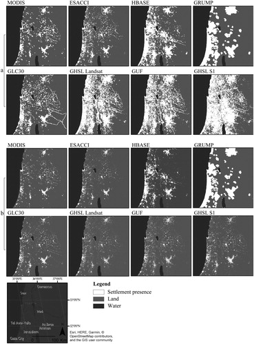
Table 1. Main characteristics of products used in the analysis.

P	D	R	MT [T/LC]	EO-s [O/R]	PC	RR	ID
MODIS 2002v5 Urban	2002	463 m	T	MODIS [O]	Urban and built-up area	10 m	Modis
GRUMP v1 Urban Extent Polygons, v1.0	1995	927 m	T	DMSP-OLS [O]	Urban extent	10 m	Grump
ESA Climate Change Initiative Land Cover v2.0.7	2015	300 m	LC	PROBA-V [O]	Urban areas	10 m	EsaCCI
GlobeLand30 2010	2010	30 m	LC	Landsat [O]	Artificial surfaces	1 m	Glc30
HBASE 2010	2010	30 m	T	Landsat [O]	Built-up And Settlement Extent	1 m	Hbase
GHS Landsat Built-up area, 2017 (*)	2014	30 m	T	Landsat [O]	Built-up area	1 m	GhsLds
GHS Sentinel 1 Built-up, 2016 (*)	2015	∼19 m	T	Sentinel 1 [R]	Built-up area	1 m	GhsS1
Global Urban Footprint 2012	2012	12 m	T	TerraSAR-X/ TanDEM-X [R]	Urban footprint	2 m	Guf12

Note: P – product designation (*some products are planned as public release in 2019); D – reference date of the layer used in this analysis; R – spatial resolution expressed in metres at the equator in a native geographic projection; MT – map type [Thematic/LandCover]; EO-s – EO programme of the main data sources producing optical or radar products [O/R]; PC – semantic of the proxy settlement class; RR – resampling resolution; ID – acronym of the derived 1 km² mask).

2.2. Generalised settlement area and agreement map

The Generalised Settlement Area concept is derived from the notion of human settlement (Stone 1965) and the operationalisation of the built-up area abstraction on metric and decametric sensor scale (Pesaresi et al. 2013). The Generalised Settlement Area is the generalisation of the built-up area abstraction to the 1 km scale. This scale corresponds to the neighbours scale or walking distance standard in the urban planning practices (IHT 2000) and is less detailed than any of the EO-derived products assessed in this study. Moreover, the Generalised Settlement Area generalises the thematic contents of the OE-derived products, leveraging on their mutual strong spatial correlation. In practice, the selected class abstractions from the EO-derived products under study are strongly correlated to the presence of built-up areas; and therefore, they are used as a proxy of the Generalised Settlement Area abstraction. The Generalised Settlement Area includes any positive evidence (i.e. logic OR) of the land cover classes associated with the presence of built-up areas and assessed by the different EO-derived product under study. As such, Generalised Settlement Area can be considered the maximum envelope in the spatial and thematic domain of the human settlement concept as assessed by remote sensing technologies at the global scale.

Any EO-derived product including class abstractions strongly correlated to the presence of built-up areas can be a source of a Generalised Settlement Area (i.e. a representation of the settlement space reality) and, by combining more than one product, we aim at better understanding of systematic disagreement and relative anomalies of the EO-derived products under study. The proposed scale of the Generalised Settlement Area allows us to consider also any product that maps settlements or urban surfaces, as we can assume that there is at least one built-up structure within 1 km² of the surface mapped by such a product. In addition, this criterion helps to mitigate (1) the spatial disagreement between OE-derived products that are not sharing the same pre-processing, geocoding and ortho-rectification of the supporting EO data; and (2) the temporal mismatch between products, as the potential new housing will occur within the vicinity of the existing settlements.

In order to create the Generalised Settlement Area, first we produce an agreement map. This map classifies each observation unit of 1 km² according to the number of products that report any existence of built-up surface or built-up surface proxy within the observation unit. Here, it will take values from zero to eight, where zero identifies areas where none of the product identifies built-up areas or proxy, and eight areas where all products have identified some. As the projection for the 1-km grid we select the World Mollweide projection, because it is an equal area projection well supported by open source processing tools, like GDAL (http://www.gdal.org/).

The procedure to generate the agreement map consists of several steps. First, we create a binary 1-km representation of each of the eight selected layers (a product settlement mask), in which the pixels with value one identify areas with presence of human settlement (and therefore the areas with at least one built-up structure), and pixels with value zero its absence. In the case of the land cover layers, we consider only those classes which approximate the presence of human settlement (the ‘artificial surface’ class of Glc30 and ‘urban areas’ class of EsaCCI). We create the eight settlement masks as follows: (1) we create a resampled binary representation of the input layer (for simplicity, we assign value zero to the ‘nodata’ pixels) by oversampling and reprojecting into the World Mollweide projection (RR in Table 1 indicates the used resampling resolution); (2) we aggregate the resulted fine resolution binary representations into a 1-km density grid; and then, (3) we generate the binary settlement masks at 1-km grid by assigning value 1 to all pixels for which the density value is greater than zero (Figure 1(a)). These eight settlement masks (ID in Table 1 introduces the acronyms to differentiate the derived masks from the main datasets) are summed into one grid – the agreement map – whose pixel value ranges from one to eight. We refer to these values agreement classes (AC), for example, a pixel classified as agreement class four (AC4) identifies an area of 1 km², where four products reported the presence of built-up area (Figure 2).

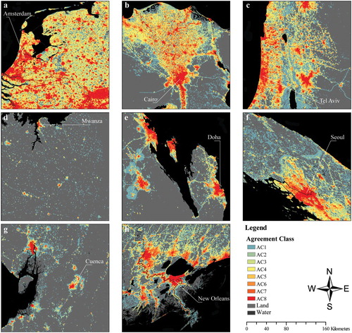
Figure 2. Examples of agreement map centred on areas nearby: Amsterdam (Netherlands) (a), Cairo (Egypt) (b), and Tel Aviv (Israel) (c); Mwanza (Tanzania) (d), Doha (Qatar) (e), and Seoul (South Korea) (f); New Orleans (USA) (g) and Cuenca (Ecuador) (h).

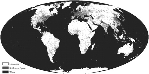
The positive domain of the agreement map, i.e. pixels with values greater than zero, constitutes the Generalised Settlement Area. The resulting Generalised Settlement Area (Figure 3) clearly differentiates the 1 km² areas where there is no evidence of settlement surface or any built-up structure in any of the input layers.

Figure 3. Overview of the Generalised Settlement Area map.

2.3. Auxiliary data

For the purpose of the presented analysis, some additional auxiliary data are created, namely the country and landmass grids, the regional aggregation of countries, and a water density map. The GADM database (https://gadm.org/) is selected as the source to produce the country 1-km grid. First, the GADM country layer (i.e. the vector layer level 0) is rasterised to the 1-km grid in World Mollweide projection, using the maximum combined area algorithm and the ‘land over water’ dominance rule. This rule results in an overestimation of the extent of countries, as all pixels of the country layer containing some land surface are classified as a country (i.e. including all pixels touched by a coastline, either inland water bodies or seas). The advantages of this approach are: (1) it reduces the discrepancies in the coastlines of the used global settlements and built-up layers, (2) it allows for accounting the surface of Generalised Settlement Area independently if it falls over the land or water. Finally, the resulted country grid is reclassified to a binary representation of landmass, named an extended landmass grid.

The country list from GADM database is mapped with the country list provided by the United Nations (UN) World Urban Prospect 2018 (UN DESA 2018), via the country ISO-3 codes presented in both datasets. All mismatches and many-to-many relations of entities are reconciled manually (with the help of information provided by UN documents, http://data.un.org/). In this way, the geographical classifications used by UN (UN sub-Regions) is applied to the country grid. The UN estimates of country total population for 2015 (https://population.un.org/wup/) are used as additional information in the regional analysis.

In the global analysis, we use a water density map to assess the impact of the method producing the landmass and country grids. This map has been produced from the Water Occurrence dataset (Pekel et al. 2016), which shows where surface water occurred between 1984 and 2015 and estimates per each 30 × 30 m pixel the overall water dynamics (i.e. water frequency: 0–100%). This dataset is used to create a water density map, which reports per each 1 km² of the Earth surface the share occupied by ‘stable’ water bodies. Only those pixels with an occurrence frequency of 80% or more are assumed to report on the presence of the ‘stable’ water (the threshold is derived through visual assessment of selected areas across the globe). First, we create a stable water mask – a binary representation of the water presence (the ‘nodata’ pixels are treated as stable water); then, we produce a 1-m water mask in World Mollweide projection (oversampling and reprojecting); finally, we aggregate it to 1-km grid estimating the surface of stable water in each 1 km² of the Earth.

3. Results

First, we perform a visual assessment. Then, the results are analysed globally and by geographic region following the UN classification of countries. We present an overall Generalised Settlement Area, the contribution of the product settlement masks to the Generalised Settlement Area, and the share of agreement class within each settlement mask.

3.1. Visual assessment

We can observe that most of the Generalised Settlement Area is concentrated in the east of North America, in Europe, India and in eastern China (Figure 3). Inspecting the agreement map (Figure 2) we note red areas (where all layers agree on the presence of built-up areas and settlements signs) surrounded by colours transiting from red, yellow to blue (a decrease in the agreement on settlement presence). These red blobs usually overlap cores of human settlements (mainly large cities). Additionally, we observe that Africa and South America show mostly low levels of agreement on the Generalised Settlement Area. A more detailed inspection of these areas reveals linear features and circles of agreement class one (AC1, blue in Figure 2(c,e)).

3.2. Global analysis

According to the resulting Generalised Settlement Area map, more than 19 million km² of the land and coastal water surface (i.e. 14.3% of the extended landmass grid) is occupied by built-up structures or located at least within 1-km of them (Table 2).

Table 2. Global assessment of water, landmass and settlement space.

	kilometre square	% over landmass	% over water (lm)
Landmass	136,324,183
water (lm)	6,468,013	4.74%
Settlement space	19,482,480	14.29%
water (SttlSpc)	529,100	0.39%	8.2%

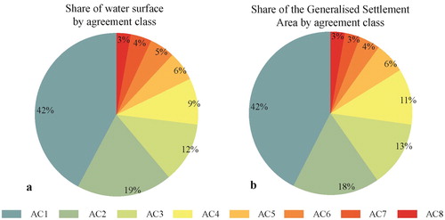
Figure 4 shows that all products agree only on 3% of the Generalised Settlement Area surface. Less than 16% of the Generalised Settlement Area surface is mapped by at least five layers, while 42% of the Generalised Settlement Area surface is the sum of separate contributions of each of the settlement masks (AC1). The water share (calculated from the water density map) in each agreement class is almost proportional to the class size and, in general, this pattern is maintained at different spatial aggregations of the Generalised Settlement Area surface. Therefore, we assume that the applied landmass generation method (i.e. systematic inclusion of coastal areas) should not influence the results.

Figure 4. Overview of the share of the agreement class within the Generalised Settlement Area map (a), and the share of the water accounted in each agreement class.

As expected, higher resolution thematic layers contribute substantially more than the other products to the Generalised Settlement Area (Table 3). The highest values of settlement mask surface are reported by GhsS1 (nearly 13 million km²), followed by Guf12 and GhsLds (nearly 10 and 9 million km², respectively). Modis represents the most conservative mapping approach, due to the used imagery and the mapping procedure, which mainly maps densely urbanised areas. Similarly, the contribution to the Generalised Settlement Area is higher from the products derived from finer resolution sensors.

Table 3. Settlement mask (SttlMsk) general statistics (AC1 – Agreement Class 1).

	SttlMsk			AC1
	Total (ths) km^2	% over landmass	% over SttlUniv	Total (ths) km^2	% over SttlMsk	share in SttlSpc AC1	share in SttlSpc
Modis	1307	1.0%	6.7%	109	8.4%	1.4%	0.31%
EsaCCI	2078	1.5%	10.7%	48	2.3%	0.6%	0.13%
Hbase	3106	2.3%	15.9%	153	4.9%	1.9%	0.43%
Grump	4457	3.3%	22.9%	958	21.5%	11.8%	2.69%
Glc30	5921	4.3%	30.4%	526	8.9%	6.5%	1.48%
GhsLds	8738	6.4%	44.9%	1672	19.1%	20.7%	4.70%
Guf12	9979	7.3%	51.2%	1264	12.7%	15.6%	3.55%
GhsS1	12,759	9.4%	65.5%	3355	26.3%	41.5%	9.43%
SttlSpc	35,586	14.29%	100%	8086	22.7%	100%	22.72%

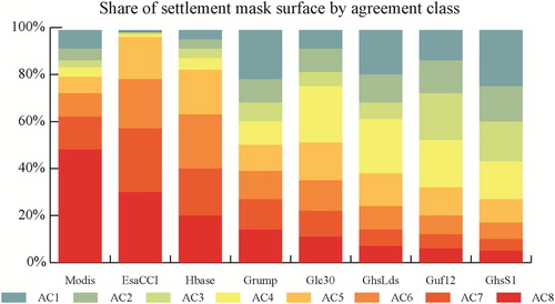
The analysis of the contribution of each layer to every agreement class is shown in Figure 5, with more details on AC1 (Table 3). 78% of the surface of the AC1 class is provided by the high-resolution thematic maps, mostly GhsS1, GhsLds and Guf12, which together map nearly 18% of the Generalised Settlement Area. Although mapping only a small subset of the Generalised Settlement Area, Modis maps only small subset of the Generalised Settlement Area surface, and only 8% of its total area is not confirmed by any other mask (which corresponds to 1.4% of the surface of the AC1). EsaCCI and Hbase products are also very conservative and map mostly the area of agreement class four or higher.

Figure 5. Overview of the share of agreement class in each settlement mask.

3.3. Geographical overview

The majority of the surface of the settlement mask falls within Asia (more than 36%), followed by Europe and North America regions (Figure 6). Noticeably, the surface of the Generalised Settlement Area in Africa is higher than the surface estimated in the Latin America and Caribbean region. When comparing the agreement class shares within the Generalised Settlement Area per region, we can observe that Oceania is the region where the layers achieve the lowest agreement, followed by Latin America and Caribbean and Africa regions (three or more products agree only in 30%).

Figure 6. Overview of the regional analysis. Total area of the Generalised Settlement Area (GSA) per UN Region in km² (a), the share of the agreement class within each region (b), and the absolute surface of each settlement masks per region (c).

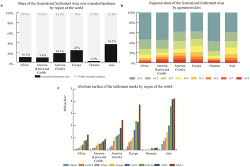
Figure 6(c) shows the absolute surface of each settlement masks per region. In general, the overall pattern is similar to the assessment at the global level. We can observe that the recent refined products have reported more Generalised Settlement Area surface compared to the other products, and GhsS1 is systematically higher in each region. The contribution of the refined grids is especially visible in Asia (almost twice as much), while GhsS1 is mapping most of the Generalised Settlement Area in Europe.

Figure 7 gathers the refined regional analysis. Here, clearly, we can observe that Northern America is closely followed by the Eastern and South-Central Asia sub-Regions for the extent of the Generalised Settlement Area surface (Figure 7(a)). The high value of Eastern Europe is explained by the fact that this region includes the Russian Federation (the Eastern Europe region has also been split into ‘Eastern Europe without Russian Federation’ and ‘Russian Federation’, marked with (*) in Figure 7). The share of the Generalised Settlement Area over the total landmass area is the highest in the European regions, with as much as 83% reported in West Europe (with Belgium reaching 93%), followed by Eastern (*) and Southern Europe.

Figure 7. Refined regional analysis of the Generalised Settlement Area (GSA) map: the total surface of the GSA per region in km² (a); the share of the GSA within surface of each region (b); and the average population density per region (PD/Lm) and GSA (PD/GSA) surfaces depicted in violet and brown colour, respectively (c). An additional division of the Easter Europe region has been made (marked by (*) symbol) to identify the Russia contribution.

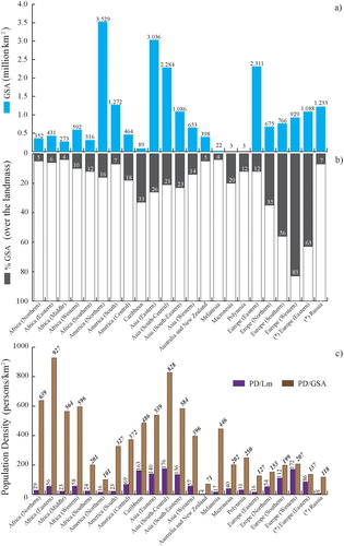
Figure 7(c) shows a comparison of the estimates of the average number of people per km² of the landmass and the Generalised Settlement Area surface per region (as reported in 2015). Noticeably, the average population density in the area of the Generalised Settlement Area is the highest in Eastern Africa, overcoming the value reported in the Southern-Central Asia sub-Region. Generally, the values for almost all African regions are very high (except for Southern Africa), with data ranges similar to those in Asian regions. Also, the Caribbean and Melanesia regions report quite high values of population density within the Generalised Settlement Area domain.

4. Discussion

According to our visual inspection, we may conclude that the selected products usually agree on the location of the large cities but do not necessarily agree on their extent. The low levels of agreement on the Generalised Settlement Area in Africa and South America could be explained by contributions of GhsS1, Guf12 and GhsLds masks, derived from products for which new methodologies were developed in order to process higher resolution imagery. These new developments resulted in improvement in the mapping of smaller settlements or probably even villages. Low levels of agreement could also be commission errors. The linear features and circles of regular shapes of agreement class one, can be explained by the semantic of GlobeLand30 (the class used as settlement proxy includes roads in the target class) and by the well-known artefacts of the GRUMP dataset – the blooming effect inherited from the nightlight data or buffering of the settlement points.

The artefacts in GRUMP and the semantic mismatch of GlobeLand30 may explain the relatively high contribution of their masks in agreement class one. MODIS seems to be the most stable product, and its mask usually indicates the areas of the highest agreement. Its presence in the area of low agreement could be explained by the oversampling method used in the production of the mask (more than 8% of Modis is not confirmed by any other mask). EsaCCI is also very conservative and maps mostly the area of agreement class four or higher. This could be explained by the ESA CCI production approach: both GUF and GHSL Landsat products were used as the sources on artificial surfaces (relying on their agreement). Noticeably, Hbase shows similar characteristics in being rather conservative in mapping the Generalised Settlement Area, despite the fact that the HBASE dataset has been derived from Landsat imagery (like GlobeLand30 or GHSL Landsat).

Regional analysis uncovers that refined resolution products report almost twice Generalised Settlement Area surface as the other products, and this can be especially appreciated in Asia. The contribution from GhsS1 is systematically higher in all regions, and the difference is more significant in Europe.

The results for the African regions indicate that there might be some issues, due to the very high value of the overall population density estimated over the Generalised Settlement Area (even higher than the values reported in Asia). These high numbers might be explained by cities and settlements with very high population densities. Harsh environmental conditions can contribute to clustering of people (and their built-up areas) over small areas (e.g. oasis); also poor areas of cities can have very high population density. However, it should not be a general trend for almost a whole continent. In fact, the Southern Africa region shows a different behaviour. One explanation could be omission errors in all products, due to the landscape and built-up area features found in these regions. Future works are needed to confirm this.

The surfaces of the Generalised Settlement Area and settlement masks reported in this work, should not be understood as an estimation of the built-up area or urban surface, neither their approximation. The Generalised Settlement Area map is an implementation of the introduced concept, and its objective is to account the overall surface in proximity to any human built-up structure (here, the distance threshold is set at 1 km). This approach may provide some overview on the land consumption by urbanisation processes ongoing currently, or that might happen in the near future. It shall be noted, that the results should be interpreted by considering the defined distance threshold, implemented via spatial unit of the settlement mask, i.e. 1 km². The change of this threshold (and therefore change of the spatial unit) will influence the results. For example, it is expected that using a distance threshold lower than 1 km; the estimated surfaces will decrease. Especially, the surfaces of the settlement masks derived from the high-resolution maps will decrease, which further will have effect on the overall estimates (in this work, these masks contribute significantly to the low-level agreement classes and explain more than 30% of the surface of the Generalised Settlement Area).

The main drawback of the proposed method is the propagation of the commission errors present in the used products, which results in an overestimation of the reported surfaces. Currently, it is not possible to evaluate this error in a traditional manner due to the lack of an appropriate validation dataset. In addition, the applied method overestimates the settlement masks produced from the coarse-resolution products, mostly due to the scale difference. The results are also affected by the implementation of the proximity rule via a 1 × 1 km grid in World Mollweide projection. Ideally, the method should be implemented using buffering techniques in equidistance projection. The temporal mismatch between the products may bias the presented results as well, because even if we assume the relative stability of the settlement extent (comparing to other geographic features like water bodies), during the past decade's urbanisation processes have become a planetary phenomenon (Melchiorri et al. 2018).

5. Conclusion

At present, according to the best global (open) knowledge available on human settlements from Earth Observation products, more than 14% of the land and coastal water surface is located in 1-km proximity of built-up structures or occupied by them. About 42% of this Generalised Settlement Area surface is derived by one global product (usually one of the fine resolution products) and not confirmed by any other. What is more, the analysis of the agreement map provides some indications that the Generalised Settlement Area in some regions (mainly in Africa) might not depict the actual situation. Future work shall seek to understand the nature of these observations. The created agreement map is a result of a straight join of the settlement masks. Different approaches for combining the masks into an agreement map can be further investigated (e.g. using majority rule, weighted union, etc.), considering the baseline layer scale, reliability or semantic. The analysis of the effects of the scale, modifiable units or aggregation method on the Generalised Settlement Area map will be part of the future work.

Despite advances in global mapping of human settlements, they remain largely unaccounted for, and we have still much to learn about their presence and extent. Our knowledge is not only incomplete when it comes to mapping the presence of small, scattered and least densely built-up settlements, but is also incomplete in terms of how to quantify the extent and density of settlements for which there is a certain degree of agreement across different products. With new remotely sensed data and processing techniques, we could improve our knowledge in this domain. As a first step, we should assess systematically where our current maps fail in representing human settlement areas (or even solitary dwellings). Currently, there is no representative reference data available necessary to perform this exercise. Secondly, future maps should provide comparable information on map quality (derived from an objective, transparent and statistical procedure designed for global geospatial information) and tools facilitating integrating and/or usage of multiple products (e.g. different versions of a product, or combining products from different providers) in a meaningful way.

Disclosure statement

No potential conflict of interest was reported by the authors.

ORCID

Aneta Jadwiga Florczyk http://orcid.org/0000-0001-8912-1500

Michele Melchiorri http://orcid.org/0000-0002-3009-8868

C. Corbane http://orcid.org/0000-0002-2670-1302

Julian Zeidler http://orcid.org/0000-0001-9444-2296

M. Schiavina http://orcid.org/0000-0003-3399-3400

S. Freire http://orcid.org/0000-0003-2282-701X

Filip Sabo http://orcid.org/0000-0003-0669-3939

Martino Pesaresi http://orcid.org/0000-0003-0620-439X

References

- Akbari, H., H. D. Matthews, and D. Seto. 2012. “The Long-Term Effect of Increasing the Albedo of Urban Areas.” Environmental Research Letters 7 (2): 024004. doi:10.1088/1748-9326/7/2/024004.
- Angel, S., J. Parent, D. L. Civco, A. Blei, and D. Potere. 2011. “The Dimensions of Global Urban Expansion: Estimates and Projections for all Countries, 2000–2050.” Progress in Planning 75: 53–107. doi:10.1016/j.progress.2011.04.001.
- Bahler, D., and L. Navarro. 2000. “ Methods for Combining Heterogeneous Sets of Classiers. 12th National Conference on Artificial Intelligence (AAAI2000).” Workshop on New Research Problems for Machine Learning.
- Bai, Y., M. Feng, H. Jiang, J. Wang, Y. Zhu, and Y. Liu. 2014. “Assessing Consistency of Five Global Land Cover Data Sets in China.” Remote Sensing 6 (9): 8739–8759. doi:10.3390/rs6098739.
- Chen, J., Y. Ban, and S. Li. 2014. “China: Open Access to Earth Land-Cover Map.” Nature 514 (7523): 434–434. doi:10.1038/514434c doi: 10.1038/nature13609
- Chen, J., J. Chen, A. Liao, X. Cao, L. Chen, X. Chen, C. He, et al. 2015. “Global Land Cover Mapping at 30 m Resolution: A POK-Based Operational Approach.” ISPRS Journal of Photogrammetry and Remote Sensing 103: 7–27. doi:10.1016/j.isprsjprs.2014.09.002.
- CIESIN, CUNY, CIDR, IFPRI, WB AND CIAT. 2017. Global Rural-Urban Mapping Project, Version 1 (GRUMPv1): Urban Extent Polygons Revision 01. Palisades, NY: NASA Socioeconomic Data and Applications Center (SEDAC).
- Corbane, C., M. Pesaresi, P. Politis, V. Syrris, A. J. Florczyk, P. Soille, L. Maffenini, et al. 2017. “Big Earth Data Analytics on Sentinel-1 and Landsat Imagery in Support to Global Human Settlements Mapping.” Big Earth Data, 1: 118–144. doi: 10.1080/20964471.2017.1397899
- Elvidge, C. D., J. Safran, I. L. Nelson, B. T. Tuttle, V. R. Hobson, K. E. Baugh, J. B. Dietz, and E. H. Erwin. 2004. “Area and Position Accuracy of DMSP Nighttime Lights Data.” In Remote Sensing and GIS Accuracy Assessment, edited by R. S. Lunetta and J. G. Lyon, 281–292. Washington, DC: CRC Press.
- ESA. 2017. Land Cover CCI, Product User Guide version 2.0 Ref. CCI-LC-PUG V 2 (UCL-Geomatics 2017).
- Esch, T., F. Bachofer, W. Heldens, A. Hirner, M. Marconcini, A. Metz-Marconcini, D. Palacios-Lopez, S. Üreyen, J. Zeidler, and S. Dech. 2018. Where we live – A summary of the achievements and planned evolution of the Global Urban Footprint. Submitted to: Remote Sensing (Special Issue Ten Years of TerraSAR-X—Scientific Results).
- Esch, T., M. Marconcini, A. Felbier, A. Roth, W. Heldens, M. Huber, M. Schwinger, H. Taubenböck, A. Müller, and S. Dech. 2013. “Urban Footprint Processor – Fully Automated Processing Chain Generating Settlement Masks From Global Data of the TanDEM-X Mission.” IEEE Geoscience and Remote Sensing Letters 10 (6): 1617–1621. doi:10.1109/LGRS.2013.2272953.
- Florczyk, A. J., S. Ferri, V. Syrris, T. Kemper, M. Halkia, P. Soille, and M. Pesaresi. 2015. “A New European Settlement Map From Optical Remotely Sensed Data.” IIEEE Journal of Selected Topics in Applied Earth Observations and Remote Sensing 9 (5): 1–15.
- Fritz, S., and L. See. 2005. “Comparison of Land Cover Maps Using Fuzzy Agreement.” International Journal of Geographical Information Science 19 (7): 787–807. doi:10.1080/13658810500072020.
- Fritz, S., L. See, C. Perger, I. McCallum, C. Schill, D. Schepaschenko, M. Duerauer, et al. 2017. “A Global Dataset of Crowdsourced Land Cover and Land Use Reference Data.” Scientific Data 4: Article no. 170075. doi:10.1038/sdata.2017.75.
- Giri, C., Z. Zhu, and B. Reed. 2005. “A Comparative Analysis of the Global Land Cover 2000 and MODIS Land Cover Data Sets.” Remote Sensing of Environment 94: 123–132. doi:10.1016/j.rse.2004.09.005.
- Gong, P., J. Wang, L. Yu, Y. Zhao, Y. Zhao, L. Liang, and J. Chen. 2013. “Finer Resolution Observation and Monitoring of Global Land Cover: First Mapping Results with Landsat TM and ETM+ Data.” International Journal of Remote Sensing 34 (7): 2607–2654. doi:10.1080/01431161.2012.748992.
- IHT. 2000. The Guidelines for Providing for Journeys on Foot. Institution of Highways and Transportation. http://www.hwa.uk.com/site/wp-content/uploads/2017/09/NR.4.3F-CIHT-Guidelines-for-Providing-Journeys-on-Foot-Chapter-3.pdf
- Kaptué Tchuenté, A. T., J.-L. Roujean, and S. M. De Jong. 2011. “Comparison and Relative Quality Assessment of the GLC2000, GLOBCOVER, MODIS and ECOCLIMAP Land Cover Data Sets at the African Continental Scale.” International Journal of Applied Earth Observation and Geoinformation 13 (2): 207–219. doi:10.1016/j.jag.2010.11.005.
- Klotz, M., T. Kemper, C. Geiß, T. Esch, and H. Taubenböck. 2016. “How Good is the map? A Multi-Scale Cross-Comparison Framework for Global Settlement Layers: Evidence From Central Europe.” Remote Sensing of Environment 178: 191–212. doi:10.1016/j.rse.2016.03.001.
- Leyk, S., J. H. Uhl, D. Balk, and B. Jones. 2018. “Assessing the Accuracy of Multi-Temporal Built-up Land Layers Across Rural-Urban Trajectories in the United States.” Remote Sensing of Environment 204: 898–917. doi:10.1016/j.rse.2017.08.035.
- Liu, X., G. Hu, Y. Chen, X. Li, X. Xu, S. Li, F. Pei, and S. Wang. 2018. “High-resolution Multi-Temporal Mapping of Global Urban Land Using Landsat Images Based on the Google Earth Engine Platform.” Remote Sensing of Environment 209: 227–239. doi:10.1016/j.rse.2018.02.055.
- McGranahan, G., D. Balk, and B. Anderson. 2007. “The Rising Tide: Assessing the Risks of Climate Change and Human Settlements in low Elevation Coastal Zones.” Environment and Urbanization 19: 17–37. doi:10.1177/0956247807076960.
- Melchiorri, M., A. J. Florczyk, S. Freire, and T. Kemper. 2018. “Unveiling 25 Years of Planetary Urbanization with Remote Sensing: Perspectives From the Global Human Settlement Layer.” Remote Sensing 10 (5): 768. doi:10.3390/rs10050768.
- Messina, J. P., M. U. G. Kraemer, O. J. Brady, D. M. Pigott, F. M. Shearer, D. J. Weiss, N. Golding, et al. 2016. “Mapping Global Environmental Suitability for Zika Virus.” eLife 5: e15272. doi:10.7554/eLife.15272.
- Ouzounis, G. K., V. Syrris, and M. Pesaresi. 2013. “Multi-scale Evaluation of Global Human Settlement Scenes Against Reference Data Using Statistical Learning.” Pattern Recognition Letters 34 (14): 1636–1647. doi:10.1016/j.patrec.2013.04.004.
- Pekel, J.-F., A. Cottam, N. Gorelick, and A. S. Belward. 2016. “High-resolution Mapping of Global Surface Water and its Long-Term Changes.” Nature 540: 418–422. doi:10.1038/nature20584.
- Pérez-Hoyos, A., F. J. García-Haro, and J. San-Miguel-Ayanz. 2012. “Conventional and Fuzzy Comparisons of Large Scale Land Cover Products: Application to CORINE, GLC2000, MODIS and GlobCover in Europe.” ISPRS Journal of Photogrammetry and Remote Sensing 74: 185–201. doi:10.1016/j.isprsjprs.2012.09.006.
- Pesaresi, M., D. Ehrlich, S. Ferri, A. J. Florczyk, S. Freire, S. Halkia, A. M. Julea, T. Kemper, P. Soille, and V. Syrris. 2016a. Operating procedure for the production of the Global Human Settlement Layer from Landsat data of the epochs 1975, 1990, 2000, and 2014. Publications Office of the European Union, EUR 27741 EN.
- Pesaresi, M., D. Ehrlich, A. J. Florczyk, S. Freire, A. Julea, T. Kemper, P. Soille, and V. Syrris. 2015. GHS built-up grid, derived from Landsat, multitemporal (1975, 1990, 2000, 2014). European Commission, Joint Research Centre (JRC) [Dataset]. http://data.europa.eu/8914;h/jrc-ghsl-ghs_built_ldsmt_globe_r2015b.
- Pesaresi, M., A. Gerhardinger, and F. Kayitakire. 2008. “A Robust Built-Up Area Presence Index by Anisotropic Rotation-Invariant Textural Measure.” IEEE Journal of Selected Topics in Applied Earth Observations and Remote Sensing 1 (3): 180–192. doi:10.1109/JSTARS.2008.2002869.
- Pesaresi, M., H. Guo, X. Blaes, D. Ehrlich, S. Ferri, L. Gueguen, M. Halkia, et al. 2013. “A Global Human Settlement Layer From Optical HR/VHR RS Data: Concept and First Results.” IEEE Journal of Selected Topics in Applied Earth Observations and Remote Sensing 6 (5): 2102–2131. doi:10.1109/JSTARS.2013.2271445.
- Pesaresi, M., V. Syrris, and A. Julea. 2016b. “A New Method for Earth Observation Data Analytics Based on Symbolic Machine Learning.” Remote Sensing 8 (5): 399. doi:10.3390/rs8050399.
- Potere, D., A. Schneider, S. Angel, and D. L. Civco. 2009. “Mapping Urban Areas on a Global Scale: Which of the Eight Maps now Available is More Accurate?” International Journal of Remote Sensing 30: 6531–6558. doi:10.1080/01431160903121134.
- Sabo, F., C. Corbane, and S. Ferri. 2017. Inter-sensor Comparison of Built-up Derived From Landsat, Sentinel-1, Sentinel-2 and SPOT5/SPOT6 Over Selected Cities. Luxembourg: Publications Office of the European Union.
- Schneider, A., M. A. Friedl, and D. Potere. 2009. “A new map of Global Urban Extent From MODIS Satellite Data.” Environmental Research Letters 4 (4): 044003. doi: 10.1088/1748-9326/4/4/044003
- Stone, K. H. 1965. “The Development of a Focus for the Geography of Settlement.” Economic Geography 41 (4): 346–355. doi:10.2307/141945.
- Taubenbock, H., T. Esch, A. Felbier, A. Roth, and S. Dech. 2010. “Pattern-Based Accuracy Assessment of an Urban Footprint Classification Using TerraSAR-X Data.” IEEE Geoscience and Remote Sensing Letters 8 (2): 278–282. doi:10.1109/LGRS.2010.2069083.
- UN DESA. 2018. United Nations Department of Economic and Social Affairs/Population Division World Urbanization Prospects: The 2018 Revision. Online: https://esa.un.org/unpd/wup/Download/Files/WUP2018_Classification_of_countries.pdf.
- Wang, P., C. Huang, E. C. Brown de Colstoun, J. C. Tilton, and B. Tan. 2017. Global Human Built-up And Settlement Extent (HBASE) Dataset From Landsat. Palisades, NY: NASA Socioeconomic Data and Applications Center (SEDAC).
- Yang, Y., P. Xiao, X. Feng, and H. Li. 2017. “Accuracy Assessment of Seven Global Land Cover Datasets Over China.” ISPRS Journal of Photogrammetry and Remote Sensing 125 (Suppl. C): 156–173. doi:10.1016/j.isprsjprs.2017.01.016.
- Zhou, Y., J. S. Smith, K. Zhao, M. Imhoff, A. Thomson, B. Bond-Lamberty, G. Asrar, X. Zhang, C. He, and C. Elvidge. 2015. “A Global map of Urban Extent From Nightlights.” Environmental Research Letters 10 (5): 054011. doi: 10.1088/1748-9326/10/5/054011