A framework for mixed-use decomposition based on temporal activity signatures extracted from big geo-data

ABSTRACT

Mixed use has been extensively applied as an urban planning principle and hinders the study of single urban functions. To address this problem, it is worth decomposing the mixed use. Inspired by the concept of spectral unmixing in remote sensing applications, this paper proposes a framework for mixed-use decomposition based on big geo-data. Mixed-use decomposition in terms of human activities differs from traditional land use research, and it is more reasonable to infer the actual urban function of land. The framework consists of four steps, namely temporal activity signature extraction, urban function base curve extraction, mixed-use decomposition, and result validation. First, the temporal activity signatures (TASs) of each zone are extracted as the proxy of human activity patterns. Second, the diurnal TASs of routine activities are extracted as urban function base curves (i.e. endmembers). Third, a linear decomposition model is used to decompose the mixed use and obtain multiple results (urban function composition, dynamic activity proportions, and the mixing index). Finally, result validation strategies are concluded. This framework offers method extensibility and has few requirements for the input data. It is validated by means of a case study of Beijing, based on a social media check-in dataset.

KEYWORDS:

• Mixed use
• spatial–temporal pattern
• urban function
• human activity
• big geo-data

1. Introduction

Urban areas are composed of land parcels with diverse functions within a limited geographical space. The rational distribution of urban functions facilitates the daily living of citizens. As an attribute of land, the urban function indicates the types of potential activities in such areas. It is directly determined by human activities and also related to the land use type, which is a static attribute planned by the government. The development of information and communication technology (ICT) offers the opportunity to gain a significant amount of geo-data with fine-grained human activity information (Ratti et al. 2006). Spatial–temporal analyses of human activities based on big geo-data, such as social media check-in data (Zhan, Ukkusuri, and Zhu 2014; Deng et al. 2018; Wu et al. 2018), taxi trajectory data (Liu et al. 2016; Tao et al. 2018), and mobile phone data (Toole et al. 2012; Pei et al. 2014), benefit the understanding of socioeconomic environments (Zheng et al. 2014; Liu et al. 2015; Shaw and Sui 2018; Yuan 2018). Regarding temporal activity signatures (TASs) as the proxy of human activities, the close relationship between human activity patterns and urban functions has been recognized (Pei et al. 2014; Zhi et al. 2016; Chen et al. 2017).

To meet the daily living needs of citizens and improve urban vitality, diverse land use types are always integrated together in several adjacent land parcels (Jacobs 1961; Grant 2002). This approach mixes multiple urban functions (i.e. mixed use) and eases the traffic pressure by changing the commuting of humans (Cervero 1996; Mindali, Raveh, and Salomon 2004; Manaugh and Kreider 2013). For further understanding of the actual urban functions, it is worth decomposing the mixed use from the perspective of human activities. However, the nature of mixed use has been largely ignored in previous urban function studies, which have assumed that each zone has a single type. Even on a very fine spatial scale such as the building level (Zhong et al. 2014; Niu et al. 2017), the vertical distribution of diverse functions in buildings may be mixed. Other studies have investigated mixed use based on land use maps and points of interest (POIs) data (Long and Liu 2013; Li, Shen, and Hao 2016; Yue et al. 2017). Mixed use has been investigated from the viewpoint of land, whereas the dynamics of human activities have been ignored. Two land parcels may exhibit the same urban function composition, but the actual activity proportions are not identical at all times. Quantified dynamic activity proportions benefit the city transportation, public security, and management.

This study regards the TAS as the proxy of human activities and converts the task into curve decomposition to decompose the mixed use (Liu et al. 2015). The TASs of routine activities are stable (for example, working during daytime and sleeping at night). These can be viewed as base curves and correspond to urban functions. The decomposition process is similar to spectral unmixing in the radiometer remote sensing field (Keshava and Mustard 2002; Bioucas-Dias et al. 2012). It offers various applications, such as snow-cover mapping (Vikhamar and Solberg 2003), alteration mineral mapping (Hosseinjani and Tangestani 2011), and land-cover mapping (Elatawneh et al. 2014; Nagol et al. 2018). Based on the spectral signatures of the endmembers (pure material), the endmember abundance in each pixel can be extracted by spectral unmixing. As an analogy, mixed use can also be revealed based on the TASs of routine activities, and this study attempts to implement this idea.

In this study, we propose a framework to decompose mixed use in terms of human activities, based on big geo-data. It focuses on mixed use in urban areas and provides a means for further understanding of the urban functions. An introduction to the framework and customization strategies for experiments are provided in Section 2. The framework consists of four steps, namely TAS extraction, urban function base curve extraction, mixed-use decomposition, and result validation. In Section 3, we apply the proposed framework to social media check-in data (from Jiepang, a social platform in China), taking Beijing as the case study area. The results and contributions are summarized and discussed in Section 5.

2. Methodology

2.1. Basic concepts

Prior to providing a detailed introduction to the decomposition framework, several basic concepts used in this paper should be clearly defined. The urban function is an attribute of land and directly determined by human activities (Gao, Janowicz, and Couclelis 2017). It has various types, such as residence, education, and entertainment. As opposed to the concept of land use determined by the original planning, urban function reflects the actual activities (Zhong et al. 2014). For example, roads support the transportation, but several wide roads with less traffic also provide an area for running and support outdoor recreation. Mixed use is both an urban planning principle and a phenomenon whereby diverse urban functions are integrated. It is extensive with urbanization and even exists on the building level (Chen et al. 2017), such as shopping malls supporting business, dining, and entertainment. In this study, the urban function base curve is the TAS of routine activities with stable patterns. Each base curve corresponds to one urban function and is the pure curve for combining the blended curve (that is, the TAS of each zone). Based on the mixed-use decomposition, we further investigate the urban function in terms of three aspects (urban function composition, dynamic activity proportions, and mixing index). Urban function composition reflects the proportion of each urban function type in the zone (for example, half education and half entertainment). The function proportion is a statistical value for the corresponding activity volume in a certain spatial–temporal unit. The dynamic activity proportion reflects the diurnal pattern of activity intensity in the zone. It is calculated based on the urban function composition. The mixing index reflects the degree of urban function mixing.

2.2. Framework for mixed-use decomposition

This framework includes four steps: TAS extraction, urban function base curve extraction, mixed-use decomposition, and result validation. Given the regularity of human activities, we assume that the TAS of the routine activity (for example, working, dining, and sleeping) is stable and corresponds to the urban function. Figure 1 illustrates an overview of the framework.

Figure 1. Overview of research framework.

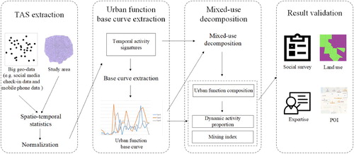
TAS extraction: The first step consists of extracting the TAS of each zone in the study area based on big geo-data, such as mobile phone data, taxi trajectory data, and social media check-in data. The spatial–temporal statistics is applicable to acquire the activity volume in each statistical unit, based on the human activity information. The definitions of spatial units and time intervals are important and depend on the data characteristics and the research objective. If the total number of spatial units is N and the dimension of the TAS is T, the TASs of all zones can be constructed as a $N\times T$ matrix. The volume of human activities in zone i during the t-th time slot is denoted by $s_i^t$, and the TAS of zone i is represented by a vector $S_i=[s_i^1,s_i^2,\dots ,s_i^T]$. To avoid differences between zones with similar activity patterns but different sizes, the vector S is normalized further (Pei et al. 2014; Liu et al. 2016).

Urban function base curve extraction: The urban function base curves can be extracted based on the TAS of each zone. Routine activities such as working and dining always occur within regular time periods, making TASs distinguishable. It should be noted that TASs of the same types may be distinctly different across cities owing to cultural diversity and time differences. Therefore, this study assumes that the routine human activity pattern is stable for each type in the area with the same life-style and uses the diurnal TASs of routine activities as the base curves of the corresponding urban functions. As a result, the observed TAS of each zone is composed of base curves. For the experimental data with activity type labels, base curves can be extracted directly by statistics. Otherwise, clustering, methods of spectral unmixing processes, and even manual sampling by expert are also practicable.

Mixed-use decomposition: Mixed-use decomposition based on the TASs and urban function base curves can produce results including urban function composition, dynamic activity proportions, and the mixing index. Considering the records of human activities are mutually independent during the TAS extraction process (namely spatial–temporal statistics), we assume that the TASs of the zones are combined by the base curves, which weighted by function proportions. The linear model for spectral unmixing (Ichoku and Karnieli 1996) is therefore used to explain the mixed mode of urban functions. The urban function composition can be obtained by solving the model. Thereafter, the other two results can be calculated based on the urban function composition of each zone.

Result validation: The urban function is an abstract concept and difficult to observe directly. In order to validate the results of the mixed-use decomposition, the data containing human activity information and other related data can be used. For global evaluation, mapping the urban function distribution and then conducting correlation analysis with other real datasets can be feasible. We can also focus on particular areas to locally validate the decomposition result by further investigation.

2.3. Customization strategies

A framework with effective applicability is required to offer optional strategies for users, which reduces the limitations of input data and extends the application field. For the proposed framework, we develop customization strategies for each step, particularly for urban function base curve extraction and result validation.

2.3.1. TAS extraction

The selections of spatial units and time intervals are key to TAS extraction. For spatial units, the optimal scales should minimize the effect of the modifiable areal unit problem (MAUP) (Openshaw and Taylor 1979). Regular grids, traffic analysis zones (TAZs), and even streets (Zhu et al. 2017) can serve as spatial units for different data. A more complex method for defining spatial units relies on the actual experimental data, such as the irregular zones created by spatial clustering, to reduce the error caused by data sparseness. For time intervals, it is necessary to meet the demand of pattern extraction as well as reduce the data sparseness error. The interval is usually set artificially (for example, an hour to create a diurnal TAS with 24 dimensions) (Pei et al. 2014). Moreover, data of weekdays and weekends/holidays are calculated separately (Frias-Martinez and Frias-Martinez 2014; Pei et al. 2014), as human activity patterns differ during these two periods in common situations.

Following the TAS extraction, normalization is a necessary step in the activity pattern study. Common normalization methods include Z-score normalization Equation (1(1) $S_i^{zscore}=[\frac{s_i^1-{\mu }_i}{{\sigma }_i},\frac{s_i^2-{\mu }_i}{{\sigma }_i},\dots ,\frac{s_i^T-{\mu }_i}{{\sigma }_i}]$(1) ), min–max normalization Equation (2(2) $S_i^{minmax}=[\frac{s_i^1-min{s}_i}{max{s}_i-min{s}_i},\frac{s_i^2-min{s}_i}{max{s}_i-min{s}_i},\dots ,\frac{s_i^T-min{s}_i}{max{s}_i-min{s}_i}]$(2) ), and sum normalization Equation (3(3) $S_i^{sum}=[\frac{s_i^1}{\sum _{j=1}^T{s}_i^j},\frac{s_i^2}{\sum _{j=1}^T{s}_i^j},\dots ,\frac{s_i^T}{\sum _{j=1}^T{s}_i^j}],$(3) ).(1) $S_i^{zscore}=[\frac{s_i^1-{\mu }_i}{{\sigma }_i},\frac{s_i^2-{\mu }_i}{{\sigma }_i},\dots ,\frac{s_i^T-{\mu }_i}{{\sigma }_i}]$(1) (2) $S_i^{minmax}=[\frac{s_i^1-min{s}_i}{max{s}_i-min{s}_i},\frac{s_i^2-min{s}_i}{max{s}_i-min{s}_i},\dots ,\frac{s_i^T-min{s}_i}{max{s}_i-min{s}_i}]$(2) (3) $S_i^{sum}=[\frac{s_i^1}{\sum _{j=1}^T{s}_i^j},\frac{s_i^2}{\sum _{j=1}^T{s}_i^j},\dots ,\frac{s_i^T}{\sum _{j=1}^T{s}_i^j}],$(3) where ${\mu }_i$ and ${\sigma }_i$ are the mean and standard deviation of the human activity volume s in zone i for every dimension (up to T), respectively.

2.3.2. Urban function base curve extraction

Methods for extracting urban function base curves depend on whether or not the activity type information is available. The former is easy to extract, as the human activity type is labeled in the actual raw data, such as the POI check-in data, trip data, and social survey data (Jiang, Ferreira, and Gonzalez 2012; Zhong et al. 2014; Zhu et al. 2015). The latter is based on unsupervised methods without activity type information. We offer three strategies below: clustering, methods of endmember extraction, and manual sampling.

Clustering: Clustering is an unsupervised method that classifies objects based on their spatial and attributive similarities, such as Euclidean distance and cosine similarity (Frias-Martinez and Frias-Martinez 2014). Several studies have used clustering to infer land use types based on TASs (Frias-Martinez and Frias-Martinez 2014; Pei et al. 2014). Clustering methods such as K-means are easy to implement and are robust in dealing with noise data. In this study, the vector of cluster centers can be regarded as the urban function base curve. However, the corresponding cluster center types are required to be labeled artificially, and the extracted base curves may still be a mixture of diverse functions.

Methods of endmember extraction: Spectral unmixing is a hot research topic that can be applied in land-cover classification (Adams et al. 1995). Endmembers are typical pixels with stable spectral signatures and cannot be divided into subclasses (for example, water, soil, and vegetation) (Bioucas-Dias et al. 2012), which are similar to urban function base curves. Thus far, numerous endmember seeking methods have been proposed, such as N-FINDR (Winter 1999), the pixel purity index method (Boardman, Kruse, and Green 1995), and SISAL (simplex identification via split augmented Lagrangian) (Bioucas-Dias 2009), which are applicable to mixed-use decomposition. Endmember extraction methods focus more on mathematical principles, rather than actual human activities. They can extract base curves with larger differences among one another and are suitable for negative situations such as outliers and the absence of pure pixels.

Manual sampling: Manual sampling is a common means of obtaining the spectral signatures of interesting objects in radiometer remote sensing. In a similar manner, the TASs of the corresponding function types can be extracted. For example, several typical restaurants may be sampled based on satellite images or city maps to obtain the TAS of the dining function. It should be noted that, in order to ensure the function purity and minimize the data sparseness effect, the sample area is required to be small and contain sufficient data for spatial statistics. A crucial factor for base curve extraction is sample selection, which is time consuming and expertise reliant. Moreover, the curve may even be adjusted flexibly based on the expertise.

In reality, it is challenging to propose a uniform quantitative indicator for method selection. The method with activity type information is easy to understand and implement, and the result is meaningful for function identification but less rigorous in mathematics. In contrast, methods of endmember extraction are types of optimization problems, which aim to minimize errors by iteration. These approaches emphasize mathematical calculation, but neglect the label of each base curve. It is also noteworthy that multi-methods may partially cover the shortcoming of each method. For example, manual sampling results can label function types using clustering results based on curve similarity.

2.3.3. Mixed-use decomposition

Mixed-use decomposition aims to provide an improved understanding of the urban function of land. Cici et al. (2015) used decomposition concepts, which are rarely applied in urban function research, to examine the seasonal and residual curve features. In this study, three indicators are obtained, namely urban function composition, dynamic activity proportions, and the mixing index.

The linear model that is used for mixed-use decomposition is simpler and more interpretable than other methods such as the neural network and nonnegative matrix factorization. Given $S_i^{mix}$ as the TAS vector for zone i, and $B_1,B_2,\dots ,B_K$ as the base curves of K functions, the linear model is formulated as Equation (4(4) $S_i^{mix}=\sum _{k=1}^K{w}_i^k{B}_k+\epsilon$(4) ).(4) $S_i^{mix}=\sum _{k=1}^K{w}_i^k{B}_k+\epsilon$(4) (5) $w_i^k\ge 0,\sum _{k=1}^K{w}_i^k=1,$(5) where ϵ is the error term and $w_i^k$ is the intensity proportion of function k within zone i. The proportion is required to satisfy the two constraints presented in Equation (5(5) $w_i^k\ge 0,\sum _{k=1}^K{w}_i^k=1,$(5) ) for physical significance. If the total number of zones is N and the curve dimension is T, Equation (4(4) $S_i^{mix}=\sum _{k=1}^K{w}_i^k{B}_k+\epsilon$(4) ) can be expressed in matrix multiplication form, as per Equation (6(6) $S_{N\times T}^{mix}=W_{N\times K}\cdot B_{K\times T}+\epsilon$(6) ). Here, $S^{mix}W$, and B are the TASs, proportions, and base curves of the urban function, respectively. An overview of the linear decomposition is illustrated in Figure 2.(6) $S_{N\times T}^{mix}=W_{N\times K}\cdot B_{K\times T}+\epsilon$(6)

Figure 2. Overview of linear decomposition.

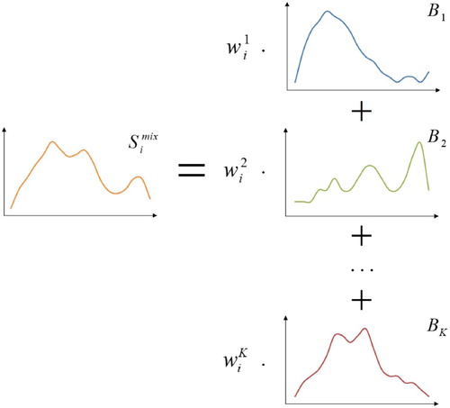
Because $S^{mix}$ and B are known variables and the error term can generally be neglected, the process of solving W can be viewed as an optimization problem for minimizing the difference between each row vector in $S^{mix}$ and $W\cdot B$ Equation (7(7) $minf(S_i^{mix},W_i\cdot B),$(7) ).(7) $minf(S_i^{mix},W_i\cdot B),$(7) where $f(X,Y)$ is the function for the vector difference measurement, and $S_i^{mix}$ and $W_i$ are the ith row vectors in the corresponding matrices. Note that the difference between two vectors $A=[a_1,a_2,\dots ,a_N]$ and $B=[b_1,b_2,\dots ,b_N]$ can be quantified by the cosine similarity Equation (8(8) $r=\frac{\sum _{i=1}^N{a}_i{b}_i}{\sqrt{\sum _{i=1}^N{a_i}^2}\sqrt{\sum _{i=1}^N{b_i}^2}}$(8) ) and root-mean-square error (RMSE) Equation (9(9) $RMSE=\sqrt{\frac{\sum _{i=1}^N(a_i-b_i{)}^2}{N}}$(9) ).(8) $r=\frac{\sum _{i=1}^N{a}_i{b}_i}{\sqrt{\sum _{i=1}^N{a_i}^2}\sqrt{\sum _{i=1}^N{b_i}^2}}$(8) (9) $RMSE=\sqrt{\frac{\sum _{i=1}^N(a_i-b_i{)}^2}{N}}$(9) As r is between 0 and 1, and a larger value reflects greater similarity between matrices, the objective is to minimize 1−r. For the RMSE, the objective is to minimize it directly.

The composition of urban functions can be regarded as a static attribute of land. In contrast, the intensity proportion of each activity is variable (Tu et al. 2017; Xing, Meng, and Shi 2018). For example, one zone may have employment and residence functions with equal proportions, but the intensities of working and sleeping are not always equal throughout the entire day. Based on the composition and base curves of the urban functions, dynamic activity proportions can be further observed.

Given $q_{ik}^t$ as the intensity proportion of the kth activity in zone i and time slot t, $p_{ik}$ as the intensity proportion of the kth function in zone i, and $B_k=[B_k^1,B_k^2,\dots ,B_k^T]$ as the vector of the kth urban function with T dimensions, the dynamic activity proportion $q_{ik}^t$ is represented by Equation (10(10) $q_{ik}^t=\frac{p_{ik}\cdot B_k^t}{\sum _{j=1}^K{p}_{ij}\cdot B_j^t}$(10) ).(10) $q_{ik}^t=\frac{p_{ik}\cdot B_k^t}{\sum _{j=1}^K{p}_{ij}\cdot B_j^t}$(10) Thereafter, the mixing index $H_i$ of zone i is calculated by the entropy model Equation (11(11) $H_i=-\sum _{k=1}^{K_i}{p}_{ik}\ln p_{ik},$(11) ) (Frank, Andresen, and Schmid 2004; Long and Liu 2013).(11) $H_i=-\sum _{k=1}^{K_i}{p}_{ik}\ln p_{ik},$(11) where $K_i$ is the number of urban function types in zone i and $p_{ik}$ is the intensity proportion of the kth function. A larger H reflects a higher mixing degree, and if zone i has only one urban function, $H_i$ is zero. In order to measure the mixed use further, Hill numbers Equation (12(12) $D_i={\left(\sum _{k=1}^{K_i}{p_{ik}}^{\alpha }\right)}^{1/(1-\alpha )},$(12) ), proposed by ecologists, are utilized to reflect the degree of richness, orderliness, and concentration (Yue et al. 2017).(12) $D_i={\left(\sum _{k=1}^{K_i}{p_{ik}}^{\alpha }\right)}^{1/(1-\alpha )},$(12) where α controls the computational content. When $\alpha =1$, Equation (12(12) $D_i={\left(\sum _{k=1}^{K_i}{p_{ik}}^{\alpha }\right)}^{1/(1-\alpha )},$(12) ) is same as the entropy model.

2.3.4. Result validation

A reasonable means of validating the mixed-use decomposition result is to investigate the actual activity intensity. However, acquiring the activity information of all citizens is difficult, and even recording details of individual activity is impossible for people themselves. Although big geo-data can provide spatial–temporal information on human activities, the activity type, which is key to inferring the urban function, is always sparse. When it is difficult to acquire real data, qualitative analysis of the urban function composition can be provided by experts. Moreover, social survey data constitute the main source for human activity research. Compared to other datasets, social survey data contain activity information with a higher quality. The questionnaire survey (on- or off-line) is a common method for collecting activity information, including, but not limited to, the starting and ending times, location, and activity type. It is noteworthy that social survey data can provide time-based activity information. The key point of the social survey is to identify sufficient users with different properties, although the process may consume substantial money and time.

Although it is challenging to use land use maps and POI data to reflect actual human activity, these are both related to the urban function. The area of each land use type can be used to reflect the corresponding function intensity, but it cannot handle spatial overlapping. In contrast, POIs have flexible shapes in order to avoid this problem, and the counting of points can be used to measure the function intensity. One limitation of POI data is the imbalance of points with different types, so the weight of each POI type is required to be set reasonably. It should be noted that, while neither land use maps nor POI data can reflect the dynamic activity proportion, they can be obtained more easily than social survey data. Furthermore, using decomposition results for other analyses provides an indirect means of validation. The mixed use exhibits relationships with several socioeconomic attributes (for example, urban vitality, building typology, and commuting mode), as proven in previous studies (Mindali, Raveh, and Salomon 2004; Ye, Li, and Liu 2018). Based on correlation analysis, the decomposition result can also be validated.

3. Case study: mixed-use decomposition based on check-in data in Beijing

3.1. Description of study area and data

To validate the proposed framework, a case study was conducted in Beijing based on social media check-in data. The data include approximately 32 million check-in records. Each record contains the record ID, geographical coordinates of the check-in points, and check-in time. Detailed information on the raw dataset is reported in Liu et al. (2014). A sample of the data is provided in Table 1. We selected only the data from weekdays (257 days in total) because the pattern of human activities on weekdays is more regular and less influenced by special circumstances such as the tourism season. The region within the 5th Ring Road in Beijing was set as the study area, as it has diverse urban functions and is appropriate for the research. TAZs were chosen as spatial units. To avoid data sparseness, zones with a low density of check-ins (one check-in per day per square kilometer at least) were eliminated. The spatial distribution of 451 zones is illustrated in Figure 3.

Figure 3. TAZs within the 5th Ring Road in Beijing.

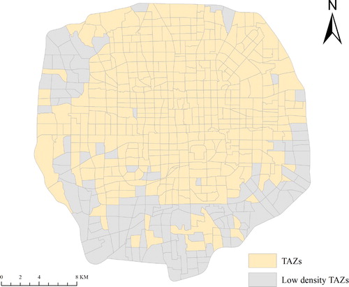
Table 1. Sample of data.

Record ID	Longitude	Latitude	Check-in time	POI type
35576021	116.3294	39.9941	2011-09-01 08:00:02	Office
35576022	116.4542	39.9348	2011-09-01 08:00:03	None
35576036	116.3530	39.9089	2011-09-01 08:00:16	School

3.2. Extraction of TASs and urban function base curves

In this research, the vector dimension is 24 with a 1-h time resolution, which has been commonly utilized in previous studies (Liu et al. 2015, 2016; Tu et al. 2017). The sum normalization method is adopted because each element is nonnegative and the element sum of each vector is equal to one. In this sense, it is suitable for the activity level study by means of hierarchical clustering (Johnson 1967; Zhu et al. 2017). The four methods mentioned in Section 2 are applied to extract the urban function base curves: K-means, SISAL ¹(Bioucas-Dias 2009), manual sampling, and statistics using POI types. The extracted base curves are illustrated in Figure 4. Note that the cluster number K = 5 for K-means is determined by silhouettes (Rousseeuw 1987), while the differences between vectors are measured by the cosine similarity. For SISAL, the number of base curves is also five for the sake of comparison. For the manual sampling, we collect samples based on satellite images and expertise. For the statistics by POI types, we combine types with similar TASs and define five urban function types: outdoor recreation, residence and transportation, dining, work and education, and entertainment. The order of these functions is consistent with the curve number in Figure 4(d). It should be noted that the manual sampling functions are the same as the above five types.

Figure 4. Urban function base curves extracted by four methods. The result of statistics by POI types is selected for the following experiment. (a) K-means, (b) SISAL, (c) manual sampling, and (d) statistics by POI types.

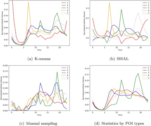
In this study, we selected the fourth group of base curves (statistics by POI types) for the following experiment. Because these are reasonable and contain the type information without manual labeling. In Figure 4(a), the curve #3 with two peaks is similar to the curve #3 in Figure 4(d). The curve #1 exhibits an abnormal peak at midnight, which may be affected by the outliers. In Figure 4(b), all curves exhibit negative values with an unknown physical significance. Apart from the curve #2, the other curves have one peak at different times, which is orthogonal but inconsistent with reality. In Figure 4(c), the curves are not smooth owing to data sparseness. The curve #2 (residence and transportation) exhibits two peaks at dinner time, which is a typical characteristic of the dining function. In Figure 4(d), the curve #3 (dining) exhibits two peaks corresponding to lunch and supper times. The curve #5 (entertainment) exhibits a peak in the evening, which also reflects reality.

3.3. Mixed-use decomposition and urban function composition analysis

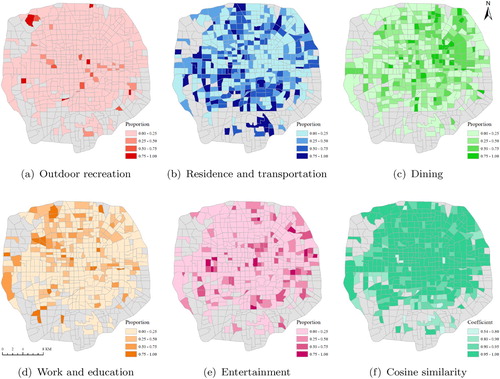
Figure 5 illustrates the urban function composition of all zones using the linear model, and the optimization evaluation using the cosine similarity. Among all of the urban functions, the proportion of outdoor recreation is lowest. Zones with high outdoor recreation intensity proportions are few and dispersed within the study area. Living at home, commuting, and dining may be the top three important activities carried out daily. For residence and transportation and dining, the zones with high proportions are nearly uniformly distributed. In Figure 5(d), most zones with high work and education proportions are in the north of Beijing, particularly the Haidian District. Owing to historical and planning reasons, many universities such as Peking University and Tsinghua University are located in Haidian. Zhongguancun, which is the industrial development zone containing Microsoft Research Asia, is also located in Haidian. The intensity proportion of entertainment is higher in the east and lower in the northwest, which is the complement of work and education to an extent. Sanlitun is located in the east of Beijing, and is the nightlife area containing numerous pubs and nightclubs. In Figure 5(f), the coefficient in the south is lower than that in the north, which is similar to the check-in data distribution. Considering that the cosine similarity may be influenced by data sparseness, we select 40 zones with coefficients less than 0.9 to verify whether a small amount of data can adequately reflect human activity patterns. The average check-in density is 4.85 (check-in counts per day per square kilometer), which is significantly lower than the average check-in density of all zones, namely 24.96.

Figure 5. Urban function composition and optimization evaluation. (a–e) Intensity proportion of each urban function, where a deeper color indicates a higher proportion. (f) Cosine similarity between TASs and combining base curves weighted by corresponding proportions. More than half of the coefficients are larger than 0.95, and few are lower than 0.80. (a) Outdoor recreation, (b) residence and transportation, (c) dining, (d) work and education, (e) entertainment, and (f) cosine similarity.

3.4. Analyses of dynamic activity proportions and mixing index

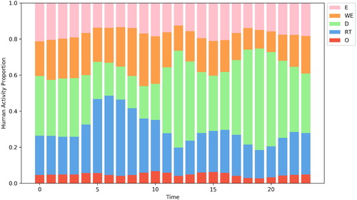
Based on the function proportion and urban function base curves, the dynamic activity proportions of each zone can be extracted Equation (10(10) $q_{ik}^t=\frac{p_{ik}\cdot B_k^t}{\sum _{j=1}^K{p}_{ij}\cdot B_j^t}$(10) ). Figure 6 illustrates the pattern of dynamic activity proportions for the entire study area. In general, the dynamic intensity proportions of different activities exhibit significant variations. Outdoor recreation has the lowest proportion and changes slightly during the day. Residence and transportation has higher proportion and is the most prominent activity during the morning, which is consistent with the nine-to-five working routine in China. Dining has the highest proportion during the day, except for the morning. The peak appears at the lunch and supper times (approximately 12:00 and 19:00, respectively), which matches the Beijing life rhythm. Work and education and entertainment have similar proportions. The trough appears at dinner time, which results from the characteristics and influence of dining.

Figure 6. Dynamic human activity proportions of the entire study area. Each color corresponds to one activity type ( outdoor recreation(O), residence and transportation(RT), dining(D), work and education(WE), and entertainment(E)). A longer bar in a certain time slot indicates a higher intensity proportion of human activities.

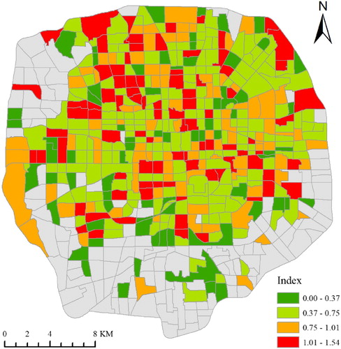
The mixing index is calculated based on the entropy model Equation (11(11) $H_i=-\sum _{k=1}^{K_i}{p}_{ik}\ln p_{ik},$(11) ). Figure 7 illustrates the spatial distribution of the mixing index in the study area. Zones with a high index are nearly randomly distributed in both the center and margin areas. This reflects the complexity of urban function research to a degree.

Figure 7. Spatial distribution of mixing index. A warmer color indicates a higher index, denoting a more diverse urban function composition.

4. Validation and discussion

4.1. Correlation analysis

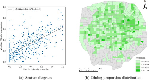
In order to validate the function proportion extracted by mixed-use decomposition, we use the POI data for comparison and take dining as an example (see Figure 8). As mentioned previously, the POIs spatial distribution can be viewed as a static attribute of land relating to the urban function. The POI proportion is calculated by the count of the corresponding POI type located in each zone, weighted by check-in volumes. The Spearman rank correlation coefficient of the two proportions exhibits a positive correlation (r=0.662, p < 0.001), indicating that the distributions in Figures 5(c) and 8(b) are similar.

Figure 8. Validation of dining proportion based on POI data. (a) Relationship between two sets of dining proportions extracted by mixed-use decomposition and POI data, respectively. Each scatter point corresponds to one zone in the study area. The gray line is the linear fitting result. (b) Distribution of dining proportion based on POI data. A deeper color indicates a higher proportion.

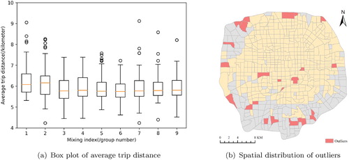
Highly mixed use tends to shorten the commuting distance (Cervero 1996). On this basis, we calculate the average trip distance (a replacement of the commuting distance) for each zone using taxi origin and destination (OD) point data acquired over one year to validate the mixing index. The trip is included only if the origin point is within the zone. As multiple factors may affect the trip distance, we divide total of 451 zones (ordered by mixing index) into 9 groups with equal counts (the final group has one more) to remove outliers. Figure 9 presents the box plot (Tukey boxplot²) of the average trip distances and spatial distribution of the outliers. The majority of outliers are located in the margin of the study area, which reflects that these long-distance trips are affected by the zone positions. Outliers located in the heartland include transportation junctions (for example, Beijing Railway Station) and scenic spots (such as Temple of Heaven Park), reflecting that zones with special functions have larger influence ranges. When removing the outliers, the Spearman rank correlation coefficient of the mixing index and average trip distances exhibits a weak negative correlation (r=−0.114, p = 0.018). This provides weak evidence and verifies the mixing index indirectly. The non-significant relationship may be affected by the bias of the taxi OD data. Other trip modes, such as walking, cycling, and public transport, are not included. Moreover, the trip distance differs from the commuting distance.

Figure 9. Validation of mixing index based on taxi OD data. (a) Box plot of average trip distance based on nine zone groups ordered by mixing index (from lowest to highest). Outliers are displayed as circle points. The light-colored line indicates the median of each group. (b) Spatial distribution of outliers.

4.2. Zooming into sample zones

In order to gain an improved understanding of the urban function composition and dynamic activity proportions, we select three zones with different urban functions as cases for detailed analyses. Figure 10 illustrates the locations and urban function compositions of the three zones. Zone A is located within Finance Street, which is the functional zone for the financial industry, planned by the government in Xicheng District. Zone B is located within Houhai, which is a tourist area in Beijing. Zone C is the main campus of Peking University, one of the oldest universities in China. In general, these zones are the employment, tourist, and education areas, respectively. However, the urban functions of these zones are mixed in different manners. In zone A, residence and transportation has the largest proportion, dining and work and education have medium proportions, outdoor recreation has a small proportion, and entertainment almost disappears. Zone B exhibits a relatively balanced urban function composition, while dining and entertainment have higher proportions. The urban function composition of zone C is similar to that of zone A, except for the existence of entertainment and the absence of outdoor recreation.

Figure 10. Location and urban function composition of three sample zones. (a) The locations of zones A to C are displayed as polygons with thick outlines. (b) Urban function composition of zones A to C. Each color corresponds to one function type. A longer bar indicates a higher function intensity proportion.

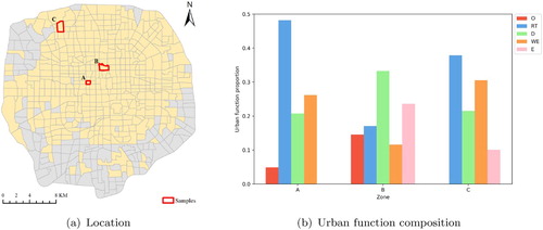
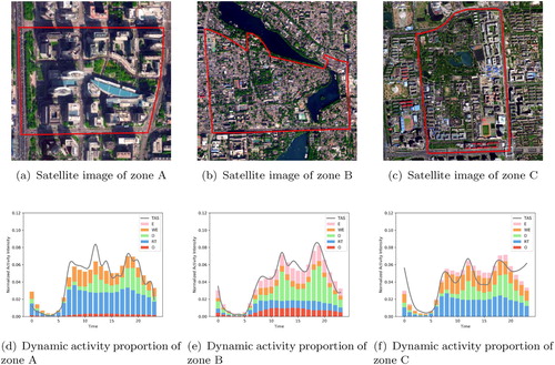
Figure 11 illustrates the satellite images and dynamic activity proportions of the three sample zones. Based on the satellite images, we find that the three zones have different sizes and shapes and contain buildings with different structures and distributions. In zone A, the intensities of residence and transportation and work and education remain almost unchanged during the daytime and decline slowly from the evening. Most of the high-rise buildings within zone A are office buildings and hotels, which support work and education and residence and transportation. Zone B has the largest size and the most balanced function composition. Although it is located within a tourist area and has many scenic spots with supporting facilities, it also contains other buildings such as schools, companies, and dwellings. The intensities of residence and transportation and work and education are lower than outdoor recreation, dining, and entertainment. Residence and transportation exhibits no peak in the morning, which may reveal that the time of tourists arriving is dispersive. Entertainment declines slowly and exists even at midnight owing to pubs. The diurnal dynamic activity proportions of zone C are similar to those of zone A. The difference is the existence of entertainment and the absence of outdoor recreation. Teaching and laboratory buildings, dormitory buildings, and dining halls within the zone C support work and education, residence and transportation, and dining, respectively.

Figure 11. Satellite images and dynamic activity proportions of three sample zones. (a–c) Satellite images (from AMAP, a mapping company in China) of zones A to C. The transparent polygon indicates the boundary of each zone. (d–f) Dynamic activity proportions of zones A to C. Each color corresponds to one activity type. A longer bar indicates a higher intensity. The gray curve illustrates the TAS of each zone. It can be viewed as the proxy of actual human activities, and is similar to the sum of all the bars (i.e. combining base curves). Note that the acronym for each human activity in the legend is the same as in Figure 6.

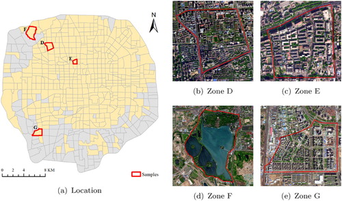
In order to compare the differences between zones with high- and low-mixing indexes further, we select zones D and E with a high-mixing index (1.340 and 1.114), and zones F and G with a low-mixing index (both 0.001) as examples (see Figure 12). Zone D contains the main campus of the Renmin University of China and a number of residential communities. Zone E is within Xinjiekou. Buildings in zone E include residential buildings, administrative buildings, and shopping malls. Zone F is Summer Palace, which belongs to the World Cultural Heritage. Zone G, containing numerous office buildings, is located in the Fengtai Science Park. Zones D and E have a higher mixing index for diverse functions such as dining, dwelling, and shopping. In contrast, zones F and G have a lower mixing index for a single function (tourism and work). The comparison demonstrates that the mixing index based on the urban function composition is reasonable.

Figure 12. Locations and satellite images of four sample zones. (a) The locations of zones D to G are displayed as polygons with thick outlines. (b–e) Satellite images (from AMAP) of zones D to G. Transparent polygons indicate the zone boundaries.

5. Conclusions and future work

This paper presented a novel framework for mixed-use decomposition in terms of human activities. This is beneficial to understanding human activity patterns and the urban function layout, as well as supporting urban management and planning. As opposed to conventional methods, the proposed framework decomposes mixed use using human activity information extracted from big geo-data. It provides a practice for applying remote sensing methods in socioeconomic environmental research. In addition to the urban function composition and mixing index, the framework can provide the dynamic activity proportions of each zone. It considers the dynamic changes in human activities, which is consistent with reality. This framework is flexible and applicable to various types of input data, provided that the TASs can be extracted. It offers several strategies for each step to match the data characteristics and research objective.

Several previous studies have considered land parcels as documents, where the function type corresponds to the document topic (Yuan, Zheng, and Xie. 2012; Gao, Janowicz, and Couclelis 2017; Yao et al. 2017). In this manner, probabilistic topic models such as latent Dirichlet allocation can be applied to urban research. One advantage of such methods is that they can extract multiple features for each land parcel, as with labeling a document from different aspects. In contrast, the framework proposed in this paper refers to the concept of spectral unmixing in radiometer remote sensing. Based on the stable pattern of routine activities, it decomposes the TAS of each zone. Our framework considers human activity dynamics, which has rarely been mentioned in previous studies (Tu et al. 2017; Xing, Meng, and Shi 2018). It offers us the opportunity to obtain detailed information on mixed use.

The case study in this paper uses a single dataset, which is easy to process but may result in errors owing to data bias. For check-in data, people tend to check-in at restaurants and stores, while they hardly check-in at their apartments. This weakens the intensity of dwelling activities objectively. In order to alleviate the shortage of single data, a number of previous studies have used multi-source data for urban function research (Hu et al. 2016; Liu et al. 2017, 2018; Tu et al. 2017). Each data type offers advantages; for example, survey and check-in data contain information on activity types, while mobile phone positioning data can support location information of people, even during the night. Combining multi-source data in a reasonable manner may allow the data to complement and reinforce one another. For the proposed framework, various data can be used as long as the TAS of each zone can be extracted. It provides numerous perspectives for analyzing the mixed use based on different input data. The framework also suits multi-source data. A simple approach is to combine the TASs extracted from different data and then add the vector dimension.

Moreover, this paper assumes that the TAS is always stable for a particular activity. However, under certain circumstances, activities of the same type may have different TASs with different locations. For example, a shopping mall located downtown and an outlet located in the suburbs provide different shopping environments (such as business hours) and lead to different TASs. In order to address this problem, we can either divide the business function into two sub-functions: downtown and suburban business, or narrow the study area to reduce the spatial difference. Furthermore, different human activities may have similar TASs. For example, many fast food restaurants remain open even at midnight. Their TASs for dining exhibit a peak at night, which is similar to the entertainment TAS. Therefore, street view and POI data are both useful for distinguishing restaurants and entertainment venues.

Regarding the method, data, and prior assumptions of this framework, our future work will focus on two aspects. The first is to determine a robust means of extracting TASs based on multi-source data. Advanced methods on feature dimension reduction, feature selection, and deep learning will be applied. This can increase the reliability of mixed-use decomposition. The second is to conduct research on the national scale, with the aim of revealing and quantifying the TAS differences with the same function type in different cities (Ahas et al. 2015). On this basis, we may obtain interesting results on the urban structure and life rhythm of citizens.

Acknowledgments

The authors would like to thank L. Gong, L. Shi and J. Wang for their advices and the anonymous reviewers for their valuable comments.

Disclosure statement

No potential conflict of interest was reported by the authors.

ORCID

Ximeng Cheng http://orcid.org/0000-0001-9923-7240

Di Zhu http://orcid.org/0000-0002-3237-6032

Chaogui Kang http://orcid.org/0000-0002-0122-9419

Zhou Huang http://orcid.org/0000-0002-1255-1913

Yu Liu http://orcid.org/0000-0002-0016-2902

Additional information

Funding

This work was supported by the National Key R&D Program of China [grant number 2017YFB0503602], the National Natural Science Foundation of China [grant numbers 41830645, 41625003, and 41771425], Strategic Priority Research Program of the Chinese Academy of Sciences [grant number XDA19040402].

Notes

1 http://www.lx.it.pt/~bioucas/code/sisal_demo.zip

2 https://en.wikipedia.org/wiki/Box_plot

References

- Adams, J. B., D. E. Sabol, V. Kapos, R. Almeida Filho, D. A. Roberts, M. O. Smith, and A. R. Gillespie. 1995. “Classification of Multispectral Images Based on Fractions of Endmembers: Application to Land-Cover Change in the Brazilian Amazon.” Remote Sensing of Environment 52 (2): 137–154.
- Ahas, R., A. Aasa, Y. Yuan, M. Raubal, Z. Smoreda, Y. Liu, C. Ziemlicki, M. Tiru, and M. Zook. 2015. “Everyday Space-Time Geographies: Using Mobile Phone-Based Sensor Data to Monitor Urban Activity in Harbin, Paris, and Tallinn.” International Journal of Geographical Information Science 29 (11): 2017–2039.
- Bioucas-Dias, J. M. 2009. “A Variable Splitting Augmented Lagrangian Approach to Linear Spectral Unmixing.” In 2009 First Workshop on Hyperspectral Image and Signal Processing: Evolution in Remote Sensing, Grenoble, France, 1–4. IEEE
- Bioucas-Dias, J. M., A. Plaza, N. Dobigeon, M. Parente, Q. Du, P. Gader, and J. Chanussot. 2012. “Hyperspectral Unmixing Overview: Geometrical, Statistical, and Sparse Regression-Based Approaches.” IEEE Journal of Selected Topics in Applied Earth Observations and Remote Sensing 5 (2): 354–379.
- Boardman, J. W., F. A. Kruse, and R. O. Green. 1995. “Mapping Target Signatures via Partial Unmixing of AVIRIS Data.” In Summaries of the Fifth Annual JPL Airborne Earth Science Workshop, Vol. 1: AVIRIS Workshop, Pasadena, CA, 23–26
- Cervero, R. 1996. “Mixed Land-Uses and Commuting: Evidence from the American Housing Survey.” Transportation Research Part A: Policy and Practice 30 (5): 361–377.
- Chen, Y., X. Liu, X. Li, X. Liu, Y. Yao, G. Hu, X. Xu, and F. Pei. 2017. “Delineating Urban Functional Areas with Building-Level Social Media Data: A Dynamic Time Warping (DTW) Distance Based K-Medoids Method.” Landscape and Urban Planning 160: 48–60.
- Cici, B., M. Gjoka, A. Markopoulou, and C. T. Butts. 2015. “On the Decomposition of Cell Phone Activity Patterns and their Connection with Urban Ecology.” In Proceedings of the 16th ACM International Symposium on Mobile Ad Hoc Networking and Computing, Hangzhou, China, 317–326. ACM
- Deng, C., W. Lin, X. Ye, Z. Li, Z. Zhang, and G. Xu. 2018. “Social Media Data as a Proxy for Hourly Fine-Scale Electric Power Consumption Estimation.” Environment and Planning A: Economy and Space. 0308518X18786250.
- Elatawneh, A., C. Kalaitzidis, G. P. Petropoulos, and T. Schneider. 2014. “Evaluation of Diverse Classification Approaches for Land Use/Cover Mapping in a Mediterranean Region Utilizing Hyperion Data.” International Journal of Digital Earth 7 (3): 194–216.
- Frank, L. D., M. A. Andresen, and T. L. Schmid. 2004. “Obesity Relationships with Community Design, Physical Activity, and Time Spent in Cars.” American Journal of Preventive Medicine 27 (2): 87–96.
- Frias-Martinez, V., and E. Frias-Martinez. 2014. “Spectral Clustering for Sensing Urban Land Use Using Twitter Activity.” Engineering Applications of Artificial Intelligence 35: 237–245.
- Gao, S., K. Janowicz, and H. Couclelis. 2017. “Extracting Urban Functional Regions from Points of Interest and Human Activities on Location-Based Social Networks.” Transactions in GIS 21 (3): 446–467.
- Grant, J. 2002. “Mixed Use in Theory and Practice: Canadian Experience with Implementing a Planning Principle.” Journal of the American Planning Association 68 (1): 71–84.
- Hosseinjani, M., and M. H. Tangestani. 2011. “Mapping Alteration Minerals Using Sub-Pixel Unmixing of ASTER Data in the Sarduiyeh Area, SE Kerman, Iran.” International Journal of Digital Earth 4 (6): 487–504.
- Hu, T., J. Yang, X. Li, and P. Gong. 2016. “Mapping Urban Land Use by Using Landsat Images and Open Social Data.” Remote Sensing 8 (2): 151.
- Ichoku, C., and A. Karnieli. 1996. “A Review of Mixture Modeling Techniques for Sub-Pixel Land Cover Estimation.” Remote Sensing Reviews 13 (3-4): 161–186.
- Jacobs, J. 1961. The Death and Life of American Cities. New York: Vintage.
- Jiang, S., J. Ferreira Jr., and M. C. Gonzalez. 2012. “Discovering Urban Spatial-Temporal Structure from Human Activity Patterns.” In Proceedings of the ACM SIGKDD International Workshop on Urban Computing, Beijing, China, 95–102. ACM
- Johnson, S. C. 1967. “Hierarchical Clustering Schemes.” Psychometrika 32 (3): 241.
- Keshava, N., and J. F. Mustard. 2002. “Spectral Unmixing.” IEEE Signal Processing Magazine 19 (1): 44–57.
- Li, M., Z. Shen, and X. Hao. 2016. “Revealing the Relationship between Spatio-Temporal Distribution of Population and Urban Function with Social Media Data.” GeoJournal 81 (6): 919–935.
- Liu, X., J. He, Y. Yao, J. Zhang, H. Liang, H. Wang, and Y. Hong. 2017. “Classifying Urban Land Use by Integrating Remote Sensing and Social Media Data.” International Journal of Geographical Information Science 31 (8): 1675–1696.
- Liu, X., C. Kang, L. Gong, and Y. Liu. 2016. “Incorporating Spatial Interaction Patterns in Classifying and Understanding Urban Land Use.” International Journal of Geographical Information Science 30 (2): 334–350.
- Liu, Y., X. Liu, S. Gao, L. Gong, C. Kang, Y. Zhi, G. Chi, and L. Shi. 2015. “Social Sensing: A New Approach to Understanding Our Socioeconomic Environments.” Annals of the Association of American Geographers 105 (3): 512–530.
- Liu, X., N. Niu, X. Liu, H. Jin, J. Ou, L. Jiao, and Y. Liu. 2018. “Characterizing Mixed-Use Buildings Based on Multi-Source Big Data.” International Journal of Geographical Information Science 32 (4): 738–756.
- Liu, Y., Z. Sui, C. Kang, and Y. Gao. 2014. “Uncovering Patterns of Inter-Urban Trip and Spatial Interaction from Social Media Check-in Data.” PloS ONE 9 (1): e86026.
- Long, Y., and X. Liu. 2013. “Featured Graphic. How Mixed is Beijing, China? A Visual Exploration of Mixed Land Use.” Environment and Planning A 45 (12): 2797–2798.
- Manaugh, K., and T. Kreider. 2013. “What is Mixed Use? Presenting an Interaction Method for Measuring Land Use Mix.” Journal of Transport and Land Use 6 (1): 63–72.
- Mindali, O., A. Raveh, and I. Salomon. 2004. “Urban Density and Energy Consumption: A New Look at Old Statistics.” Transportation Research Part A: Policy and Practice 38 (2): 143–162.
- Nagol, J. R., J. O. Sexton, A. Anand, R. Sahajpal, and T. C. Edwards. 2018. “Isolating Type-Specific Phenologies Through Spectral Unmixing of Satellite Time Series.” International Journal of Digital Earth11 (3): 233–245.
- Niu, N., X. Liu, H. Jin, X. Ye, Y. Liu, X. Li, Y. Chen, and S. Li. 2017. “Integrating Multi-Source Big Data to Infer Building Functions.” International Journal of Geographical Information Science 31 (9): 1871–1890.
- Openshaw, S., and P. J. Taylor. 1979. “A Million or so Correlation Coefficients: Three Experiments on the Modifiable Areal Unit Problem.” In Statistical Applications in the Spatial Sciences, 127–144.
- Pei, T., S. Sobolevsky, C. Ratti, S. Shaw, T. Li, and C. Zhou. 2014. “A New Insight into Land Use Classification Based on Aggregated Mobile Phone Data.” International Journal of Geographical Information Science 28 (9): 1988–2007.
- Ratti, C., R. M. Pulselli, S. Williams, and D. Frenchman. 2006. “Mobile Landscapes: Using Location Data from Cell Phones for Urban Analysis.” Environment and Planning B: Planning and Design 33 (5): 727–748.
- Rousseeuw, P. J. 1987. “Silhouettes: A Graphical Aid to the Interpretation and Validation of Cluster Analysis.” Journal of Computational and Applied Mathematics 20: 53–65.
- Shaw, S., and D. Sui. 2018. “GIScience for Human Dynamics Research in a Changing World.” Transactions in GIS 22 (4): 891–899.
- Tao, H., K. Wang, L. Zhuo, and X. Li. 2018. “Re-examining Urban Region and Inferring Regional Function Based on Spatial–Temporal Interaction.” International Journal of Digital Earth. doi: 10.1080/17538947.2018.1425490.
- Toole, J. L., M. Ulm, M. C. González, and D. Bauer. 2012. “Inferring Land Use from Mobile Phone Activity.” In Proceedings of the ACM SIGKDD International Workshop on Urban Computing, Beijing, China, 1–8. ACM
- Tu, W., J. Cao, Y. Yue, S. Shaw, M. Zhou, Z. Wang, X. Chang, Y. Xu, and Q. Li. 2017. “Coupling Mobile Phone and Social Media Data: A New Approach to Understanding Urban Functions and Diurnal Patterns.” International Journal of Geographical Information Science 31 (12): 2331–2358.
- Vikhamar, D., and R. Solberg. 2003. “Snow-Cover Mapping in Forests by Constrained Linear Spectral Unmixing of MODIS Data.” Remote Sensing of Environment 88 (3): 309–323.
- Winter, M. E. 1999. “N-FINDR: An Algorithm for Fast Autonomous Spectral End-Member Determination in Hyperspectral Data.” In SPIE's International Symposium on Optical Science, Engineering, and Instrumentation, 266–275. International Society for Optics and Photonics.
- Wu, C., X. Ye, F. Ren, and Q. Du. 2018. “Check-in Behaviour and Spatio-Temporal Vibrancy: An Exploratory Analysis in Shenzhen, China.” Cities 77: 104–116.
- Xing, H., Y. Meng, and Y. Shi. 2018. “A Dynamic Human Activity-Driven Model for Mixed Land Use Evaluation Using Social Media Data.” Transactions in GIS 22 (5): 1130–1151.
- Yao, Y., X. Li, X. Liu, P. Liu, Z. Liang, J. Zhang, and K. Mai. 2017. “Sensing Spatial Distribution of Urban Land Use by Integrating Points-of-Interest and Google Word2Vec Model.” International Journal of Geographical Information Science 31 (4): 825–848.
- Ye, Y., D. Li, and X. Liu. 2018. “How Block Density and Typology Affect Urban Vitality: An Exploratory Analysis in Shenzhen, China.” Urban Geography 39 (4): 631–652.
- Yuan, M. 2018. “Human Dynamics in Space and Time: A Brief History and a View Forward.” Transactions in GIS 22 (4): 900–912.
- Yuan, J., Y. Zheng, and X. Xie. 2012. “Discovering Regions of Different Functions in a City Using Human Mobility and POIs.” In Proceedings of the 18th ACM SIGKDD International Conference on Knowledge Discovery and Data Mining, Beijing, China, 186–194. ACM
- Yue, Y., Y. Zhuang, A. G. O. Yeh, J. Xie, C. Ma, and Q. Li. 2017. “Measurements of POI-Based Mixed Use and Their Relationships with Neighbourhood Vibrancy.” International Journal of Geographical Information Science 31 (4): 658–675.
- Zhan, X., S. V. Ukkusuri, and F. Zhu. 2014. “Inferring Urban Land Use Using Large-Scale Social Media Check-in Data.” Networks and Spatial Economics 14 (3-4): 647–667.
- Zheng, Y., L. Capra, O. Wolfson, and H. Yang. 2014. “Urban Computing: Concepts, Methodologies, and Applications.” ACM Transactions on Intelligent Systems and Technology 5 (3): 38.
- Zhi, Y., H. Li, D. Wang, M. Deng, S. Wang, J. Gao, Z. Duan, and Y. Liu. 2016. “Latent Spatio-Temporal Activity Structures: A New Approach to Inferring Intra-Urban Functional Regions via Social Media Check-in Data.” Geo-spatial Information Science 19 (2): 94–105.
- Zhong, C., X. Huang, S. M. Arisona, G. Schmitt, and M. Batty. 2014. “Inferring Building Functions from a Probabilistic Model Using Public Transportation Data.” Computers, Environment and Urban Systems 48: 124–137.
- Zhu, D., N. Wang, L. Wu, and Y. Liu. 2017. “Street as a Big Geo-Data Assembly and Analysis Unit in Urban Studies: A Case Study Using Beijing Taxi Data.” Applied Geography 86: 152–164.
- Zhu, Z., J. Yang, C. Zhong, J. Seiter, and G. Tröster. 2015. “Learning Functional Compositions of Urban Spaces with Crowd-Augmented Travel Survey Data.” In Proceedings of the 23rd SIGSPATIAL International Conference on Advances in Geographic Information Systems, Seattle, Washington, 22. ACM