The impact of seasonality on multi-scale feature extraction techniques

ABSTRACT

A key component in constructing a broad-scale, gridded population dataset is fine resolution geospatial data accurately depicting the extent of human activity. Analogous datasets are often developed using a wide range of methods and classification techniques, including the use of spatial features, spectral features, or the coupling of both to identify the presence of man-made structures from high-resolution satellite imagery. By using spatial and textural-based descriptors to generate high-resolution settlement layers for two dissimilar regions at the peak of seasonal disparity, this study attempts to quantify the influence of seasonality on the accuracy of a supervised, multi-scale, feature extraction framework for automated delineation of human settlement. Results generated by numerous models are evaluated against a reference dataset allowing for assessment of seasonal and feature differences in the context of accuracy. Global or regional mapping of human settlement requires the assemblage of high-resolution satellite images with variegated acquisition characteristics (season, sun elevation, off-nadir, etc.) to produce a cloud-free composite image from which features are extracted. Results of this study suggest an emphasis on imagery criteria, in particular acquisition date, could improve classification accuracy when mapping human settlement at scale.

KEYWORDS:

• Remote sensing
• high-resolution imagery
• image processing
• human settlement
• accuracy

1. Introduction

The functionality of population distribution datasets has always been evident. The availability of datasets describing population conditions at a given time has proven valuable when planning or responding to population growth and distribution as well as emergency situations that arise (Tatem and Hay 2004). The inherent difficulties associated with producing said datasets have likewise been well documented (Tatem and Hay 2004). Whether it is mapping scattered villages composed of huts in sub-Saharan Africa or documenting urban expansion in U.S. cities, extracting information from high-resolution satellite imagery associated with the extent of human activity from any landscape will be challenging. Initial obstacles encompass intrinsic questions of resolution, scale, and metadata of available imagery such as sun elevation, view angle, and acquisition date (Karim et al. 2017). The method or technique decided upon will likely present its own host of considerations as there are often drawbacks or trade-offs to appraise (Medjahed 2015). Imagery attributes relating to haze or cloud cover can make processes such as feature extraction more difficult (Bai et al. 2016; Champion 2016; Dare 2005; Li et al. 2017; Liu and Yamazaki 2012; Panem et al. 2005; Ramesh and Satheesh Kumar 2013; Sun et al. 2017; Wu et al. 2016; Wu and Tang 2005). Terrain characteristics such as ridge lines, mining sites, river beds, gullies, rocks, or confounding scrubland aspects can mimic targeted features. Local settlement characteristics can vary dramatically within a small region challenging even the best trained models. The impact of these factors is not always well defined or clearly understood. In order to aid that circumstance this study attempts to isolate a single characteristic associated with broad-scale processing of remotely sensed images. By focusing on acquisition date, more specifically seasonality, this research evaluates the potential impact seasonal variations might have on the classification accuracy of human settlement using multi-scale feature extraction techniques.

2. Background

The core concept of feature extraction or object classification is to analyze the elements of image components in order to assign said components a label or assemble them into categories for further applications (Medjahed 2015). Contemporary methods or techniques have evolved to incorporate a proliferation of commercially available high-resolution imagery. Methods in the field have also incorporated technological advancements in the form of machine learning, high performance computing (HPC), and scalability (Alvarez-Cedillo 2013; Cheriyadat et al. 2007; Chen, Li, and Lin 2011; Hirabayashi et al. 2013; Patlolla et al. 2015; Prisacariu and Reed 2009; Storcheus, Rostamizadeh, and Kumar 2015). The feature extraction process utilized in this study was developed at ORNL and incorporates the parallel computing platform CUDA to leverage GPU capabilities (Cheriyadat et al. 2007). A commonality among recent techniques is the use of object-based classification methods over pixel-based methods as this makes better use of the details provided by high-resolution imagery as well as incorporating a spatial aspect that has proven to be beneficial (Crommelinck et al. 2016).

Coupled with the philosophy of supervised learning, support vector machines (SVM) accomplish classification via mapping to feature space and compare favorably with other commonly used classifiers (Bosch, Zisserman, and Munoz 2007; Kim, Kim, and Savarese 2012; Qian et al. 2015; Wainberg, Alipanahi, and Frey 2016; Wen et al. 2018). One of the benefits this method offers is the ability to adequately generalize from a less than ideal training set (Crommelinck et al. 2016). SVMs provide the capability to incorporate a number of different feature types and can be leveraged for a variety of different applications. In this study the SVM was constructed to operate at a 16 by 16 pixel block level. The classifier determined whether the pixel blocks are considered settlement or non-settlement based on the feature descriptors generated. This was achieved by incorporating Python, CUDA, and C++ to employ the algorithms within an HPC framework described in Cheriyadat et al. (2007) and Patlolla et al. (2015). Spectral characteristics of pixels along with spatial information regarding features were used to make this determination. This process was performed at multiple scales, five in total, scaling up from the original 16 by 16 pixel block to maximize the contextual information possibly associated with each feature (Weber et al. 2018).

Utilizing contemporary methodologies this study aims to evaluate the impact seasonality might have on multi-scale feature extraction techniques. Replication of a general workflow centered around a supervised SVM classifier provides an adequate number of samples to imply the significance of any trends observed. By evaluating results in the context of a comprehensive comparison as well as individual features, the seasonal impact is isolated from the feature idiosyncrasies and an overview of expectations with regards to conventional techniques is achievable.

3. Study area

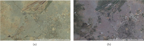
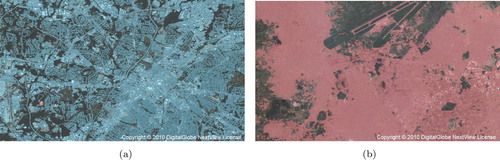
Two regions were selected to assess a range of seasonal effects in notably disparate settings. The regions of study were Charlotte, North Carolina (United States) and Kano, Nigeria. Charlotte is a city with over 800,000 people spread across approximately 770 square kilometers (Bureau 2016). This city resides in a humid subtropical region (Peel, Finlayson, and McMahon 2007) that experiences a wide range of temperatures throughout the year with four distinct seasons: spring, summer, fall, and winter. April is the driest month while summer is typically humid and hot compared to the winters that are generally short and cool (Figure 1). Kano is a city with almost three million people spread across less than 500 square kilometers (Ayila, Oluseyi, and Anas 2014). Occupying a tropical savanna region (Peel, Finlayson, and McMahon 2007), Kano is typically very hot throughout the year and experiences two distinct seasons; a dry and wet season (Figure 2). December through February tends to be comparatively cool and very dry while the vast majority of the region's precipitation is received between the months of June and September. These two locations offer distinct seasonal variations that could impact supervised, multi-scale, feature extraction results.

Figure 1. Example of seasonal differences for Charlotte, North Carolina (United States) imagery. (a) Charlotte 01/24/2016 (Winter Season) and (b) Charlotte 07/05/2016 (Summer Season).

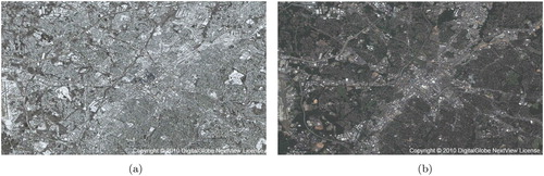
Figure 2. Example of seasonal differences for Kano, Nigeria imagery. (a) Kano 01/27/2014 (Dry Season) and (b) Kano 08/29/2014 (Wet Season).

For both regions, WorldView-2 and WorldView-3 imagery was acquired from DigitalGlobe under the Nextview License agreement (DigitalGlobe 2017). A total of eight images were selected; four different dates within a 12-month period for each region. Images were explicitly selected so that acquisition dates coincided with the approximate peak of each of the four seasons in Charlotte and two seasons in Kano, as well as two midpoints between the two dominant seasons in Kano (Table 1). Images selected for the region of analysis were multispectral pan-sharpened (RBG-NIR) with a spatial resolution of 0.5 meter and unobstructed by clouds.

Table 1. Imagery collection parameters.

Study Area	Month	Day	Year	Season	Sensor	Cell size
Charlotte	January	24	2016	Winter	WV02	4.5e−06, 4.5e−06
Charlotte	April	04	2016	Spring	WV02	4.5e−06, 4.5e−06
Charlotte	July	05	2016	Summer	WV02	4.5e−06, 4.5e−06
Charlotte	October	10	2016	Fall	WV02	4.5e−06, 4.5e−06
Kano	January	27	2014	Dry	WV02	4.5e−06, 4.5e−06
Kano	May	02	2014	Midpoint	WV02	4.5e−06, 4.5e−06
Kano	August	29	2014	Wet	WV02	4.5e−06, 4.5e−06
Kano	November	26	2014	Midpoint	WV03	3.6e−06, 3.6e−06

4. Methods

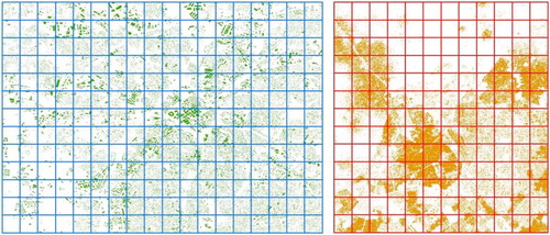
An arbitrary grid of uniform, non-overlapping training blocks was generated for each study area where each training block spanned 2048 by 2048 pixels. Due to varying degrees of swath orientation for each image, the previously described tiling scheme was only generated where all four images coincided. This created a grid of 234 training blocks for Charlotte and 156 for Kano, totaling approximately 200 square kilometers and 160 square kilometers respectively (Figure 3).

Figure 3. Charlotte and Kano training blocks along with reference data (building features).

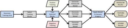
Fifteen training blocks from a study area's training grid were randomly selected. The reference building features from each training block were used as positive training and the remaining area was used as negative training. Low-level image features were then extracted for the 15 training blocks (Figure 4). Features included histogram of oriented gradients and the gray level co-occurrence matrix (HOGGLCM), textons (TEXTONS), and vegetation indices (VEGIND).

Figure 4. Example of feature extraction during model creation for Charlotte 07/05/2016 image. (a) Isolated area downtown and (b) HOGGLCM extracted features for the area.

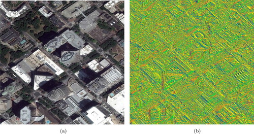
HOGGLCM is the concatenation of two independent features and can be described as a texture-based feature combining the use of filters and pixel values to identify/characterize spatial structure and composition (Dalal and Triggs 2005; Patlolla et al. 2012) TEXTONS is similar to HOGGLCM and functions by utilizing filters for the purpose of capturing textural variation and orientation (Malik et al. 2001; Patlolla et al. 2015) Differing from both HOGGLCM and TEXTONS is VEGIND, which derives a variety of spectral indices and concatenates each individual index into a single feature vector (see Appendix A, Table A1) to differentiate vegetation from non-vegetation.

Once information had been extracted for each of the three features, this was then input to a linear SVM to generate a binary classification model for each feature (Figure 5). This was accomplished by mapping the feature vector to one of the binary classes (settlement and non-settlement) in multidimensional space where the SVM could locate the hyperplane that best represents the boundary between the two classes (Kim, Kim, and Savarese 2012). In turn, each model was applied to the entire image to produce a binary output representing the presence/absence of human settlement (Figure 6). For further information regarding the HPC strategy employed for this process consult Patlolla et al. (2012) and for a detailed description of the work flow refer to Weber et al. (2018). This entire process was reproduced 20 times for each of the four seasonal images. Therefore, a total of 240 binary classifications were generated for each study region. During each iteration, a new training sample consisting of 15 blocks was randomly selected.

Figure 5. Charlotte January feature run example.

4.1. Metrics

The 240 classified maps for Charlotte were compared on a pixel by pixel basis against LiDAR (Light Detection and Ranging) derived building features with a spatial resolution of 0.5 meters (Government 2013). The 240 classified maps for Kano were compared on a pixel by pixel basis with building features produced by deep convolutional neural networks (CNNs) with a spatial resolution of 0.5 meter (Yuan et al. 2018). These CNNs utilized volunteered geographic information building outlines as training and generated a data set with impressive validation results that could be considered comparable to those of LiDAR building features. Comparisons for both study areas were performed at the native spatial resolution of that particular image (Table 1). For example, the results for Charlotte January imagery were generated at the same spatial resolution (cell size) as the imagery itself and compared to a reference dataset of the same resolution. The assessment was accomplished by calculating a precision, recall, and F1 score for each result. Precision provides a useful metric for evaluating the effectiveness of a model in positive identification, in this case highlighting how much settlement commission was present in the results (1). Recall is more useful for appraising sensitivity or in this study the omission of settlement (2). The F1 score takes into account precision along with recall in order to evaluate the model performance in a more balanced manner that can be best described as the harmonic mean of the two (3). These metrics are commonly used to assess the performance of a process that generates discrete results and were chosen for their effectiveness in representing the basic form model error present in this study (Buckland and Gey 1994; Derczynski 2016; Flach and Kull 2015; Goutte and Gaussier 2005; Olson and Delen 2008; Torgo and Ribeiro 2009; Saito and Rehmsmeier 2015).(1) $Precision=NumberCorrectSettlementPixels/TotalNumberClassifiedSettlementPixels$(1) (2) $Recall=NumberCorrectSettlementPixels/TotalNumberReferenceSettlementPixels$(2) (3) $F1Score=2x\left(Precison/Recall\right)/(Precision+Recall)$(3)

5. Results

5.1. Significance of comprehensive results

A Kruskal–Wallis one-way ANOVA on ranks test was performed to assess whether any differences in results were statistically significant. This test was chosen over the parametric equivalent, one-way ANOVA, after a Shapiro–Wilk's test for normality confirmed the data were not normally distributed. To comprehensively assess seasonal differences in classification accuracy for each study region, accuracy metrics of the 240 classified maps were evaluated together using season as the random factor (Table 2). For Charlotte, each measure of accuracy produced a p-value equivalent to zero. As these results were well below the 0.05 threshold associated with a 95% confidence level, this suggests there are significant differences in classification performance across seasons for each accuracy measure in Charlotte. For Kano, recall was the only metric in which significant differences can be seen among the seasons (Table 2). Similarly, to determine whether any significant differences exist between classification performance and each feature, the 240 classified maps were evaluated together using the extracted feature as the random factor (Table 2). For both Charlotte and Kano, all accuracy metrics showed statistically significant differences between measured accuracy and the feature used to classify that image.

Table 2. Significance of comprehensive differences.

Study area	Factor	Metric	p-Value
Charlotte	Seasons	Precision	0.00
Charlotte	Seasons	Recall	0.00
Charlotte	Seasons	F1 Score	0.00
Kano	Seasons	Precision	0.51
Kano	Seasons	Recall	0.02
Kano	Seasons	F1 Score	0.51
Charlotte	Features	Precision	0.00
Charlotte	Features	Recall	0.00
Charlotte	Features	F1 Score	0.00
Kano	Features	Precision	0.00
Kano	Features	Recall	0.00
Kano	Features	F1 Score	0.00

5.2. Significance of individual results

To conduct a more detailed and focused analysis, individual features were isolated in order to identify any potential differences in classification accuracy of a single feature across multiple seasons (Table 3). Except for the combination of TEXTONS and recall, all other possible combinations of feature type and accuracy metric were statistically significant for Charlotte. Meaning that all other features and accuracy measures significantly varied across seasons.

Table 3. Significance of individual differences.

Study area	Feature	Metric	p-Value
Charlotte	HOGGLCM	Precision	0.00
Charlotte	HOGGLCM	Recall	0.00
Charlotte	HOGGLCM	F1 Score	0.00
Charlotte	TEXTONS	Precision	0.00
Charlotte	TEXTONS	Recall	0.48
Charlotte	TEXTONS	F1 Score	0.00
Charlotte	VEGIND	Precision	0.00
Charlotte	VEGIND	Recall	0.00
Charlotte	VEGIND	F1 Score	0.00
Kano	HOGGLCM	Precision	0.43
Kano	HOGGLCM	Recall	0.20
Kano	HOGGLCM	F1 Score	0.41
Kano	TEXTONS	Precision	0.16
Kano	TEXTONS	Recall	0.50
Kano	TEXTONS	F1 Score	0.16
Kano	VEGIND	Precision	0.46
Kano	VEGIND	Recall	0.00
Kano	VEGIND	F1 Score	0.47

Conversely, seasonal differences for feature type and accuracy metric were not as pronounced for Kano. All p-values generated for HOGGLCM and TEXTONS were well above the 0.05 threshold for a 95% confidence level (Table 3). This indicates there were no significant differences in the metrics across the seasons for these two features. The same holds true for VEGIND as well with recall being the lone exception (Table 3). A possible explanation for the dissimilarity in results between the two study areas could be attributed to the difference in local settlement characteristics and terrain properties. Buildings in Charlotte appeared to be larger, more sparse, and less condensed when compared to Kano. There also appeared to be more impervious surfaces in Charlotte than Kano, which could have replicated settlement characteristics in terms of texture and shape.

5.3. Comprehensive seasonal differences

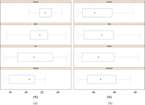
When classification results are pooled together using season as the random factor there are some notable findings. January would most likely be the optimal season in Charlotte, while October appeared to produce the worst results (Figure 7(a)). The dashed lines represent the minimum and maximum values, the box represents the interquartile range (IQR), and the dot represents the mean. One possible explanation for the January imagery producing the best results is the significant snow cover present in the imagery. This suggests the disparity in appearance between snow covered and non-snow covered areas enhanced the contrast and improved performance of each feature. Earlier statistical assessment showed there were no significant differences in the results across the seasons for Kano. This finding can be observed by the similarity in seasonal distribution of accuracy scores in (Figure 7(b)).

Figure 7. F1 score differences for seasons. (a) Charlotte F1 scores for seasons and (b) Kano F1 scores for seasons.

As a complimentary assessment of individual feature performance, results for the four seasons are pooled together and the feature type is used as a random factor. From this assessment, VEGIND certainly stands out as the better option for both study areas, while HOGGLCM appears to generate the worst results (Figure 8). TEXTONS showed noticeably better results in Charlotte, especially when compared with a similar feature HOGGLCM (Figure 8(a)). Ascribing this difference to previously mentioned local settlement characteristics or terrain properties would most likely require further research.

Figure 8. F1 score differences for features. (a) Charlotte F1 scores for features and (b) Kano F1 scores for features.

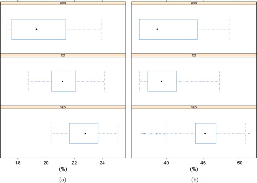
Figure 6. Example of VEGIND results. (a) Charlotte 07/05/2016 Run Number 14 and (b) Kano 08/29/2014 Run Number 9.

5.4. Seasonal impact on each feature

A final examination of seasonal results for each feature shows both similarities and differences for the two study areas. VEGIND outperforms the other two features in each instance save one, January in Charlotte (Figure 9(a)). In Charlotte both HOGGLCM and TEXTONS would best be utilized in January when snow is on the ground (Figure 9(a)). VEGIND performed best in July which corresponds to the peak of summer, when differentiating vegetation and non-vegetation would theoretically be more ideal than the other three image dates. Of note is the observable low point for results in October, corresponding to the peak of fall (Figure 9(a)). This was observed for all three features and raises questions when one takes into account that visual differences in October imagery and April imagery are minimal at best.

Figure 9. Seasonal impact on each feature. (a) Charlotte F1 score mean by season and (b) Kano F1 score mean by season.

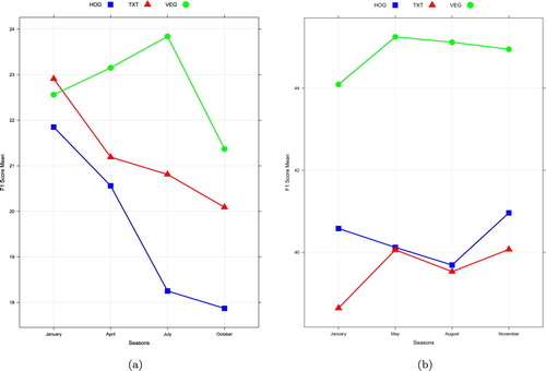
Given knowledge of Kano seasonality one would expect VEGIND to perform best in August at the peak of the wet season. However, May produced the highest score, though the difference in score between May and August was 0.13% (Figure 9(b) and Table A3). As expected VEGIND did generate the lowest F1 score in January at the peak of the dry season. HOGGLCM and TEXTONS generated their highest scores in November, which upon visual inspection would be difficult to discern from the other midpoint imagery in May. There was a noticeable difference in the January scores between the two similar features raising questions as to what factors might be influencing the results. The F1 scores, as were the precision and recall scores, were noticeably higher in Kano when compared to Charlotte which can most likely be attributed to the previously mentioned local settlement characteristics and terrain properties (Tables A2 and A3).

6. Conclusion

Though differences in accuracy metrics among the seasons and features in this study only varied from 5–10%, this seemingly small difference can have a large impact within the context of scale. When performing satellite image based feature extraction across broad countries, regions, or simply a few image strips, minor improvements in classification accuracy can have a profound impact. Tests performed on the Kano study area showed that a single percent increase in overall classification accuracy resulted in a reduction of 1.6 square kilometers of falsely classified settlement (i.e. false positive). At broader scales, this 1% increase in overall accuracy would have an even greater impact on the total area of falsely classified settlement removed. This preliminary evaluation of accuracy impact underscores the obvious need for maximizing classification results not only in the algorithm and implementation, but also in the selection criteria of potential images to process, particularly when these techniques are commonly employed in gridded population data sets, estimation of built-up area, quantifying our ecological footprint, and/or urban dynamics research.

From this research, we have determined that seasonality does influence the accuracy of multi-scale feature extraction based settlement mapping. However, the influence of seasonality was not uniform as it varied depending on the feature employed for both study regions. There are limitations to the trends observed in this study that should be noted. Charlotte and Kano share certain characteristics with other regions in terms of climate, terrain, and settlement characteristics but are by no means representative of all regions. The imagery utilized in this study was half meter multi-spectral imagery and it remains to be seen if the trends in results observed would be replicated with panchromatic imagery (which excludes the use of VEGIND) or that of a lower resolution. Three features were incorporated in this study and the unique properties associated with each suggest that other features would not necessarily be expected to show the same trends. Also of note is the three accuracy metrics utilized in this study, there are several more commonly used in the field and given the inherent differences further testing would be required to investigate potential manifestations of these variations.

However, seasonal differences were still significant enough to draw conclusions that warrant consideration. For instance, the performance of VEGIND, particularly when compared to the other two features, would appear ideally suited for regions experiencing peak disparity in vegetation and non-vegetation. The other two features, HOGGLCM and TEXTONS, also proved useful in certain situations. Their performance on the January snow covered imagery of Charlotte suggests possible applications at extreme latitudes when the acquisition of snow free imagery could be more problematic or in other areas where vegetation is more sparse (e.g. scrublands and deserts). Overall, the results of this study do highlight trends worth considering when acquiring imagery for feature extraction techniques as well as the inherent factors associated with these decisions.

Acknowledgments

This study was made possible by support and encouragement from Jeanette Weaver, Amy Rose, and fellow colleagues on the Population Distribution and Dynamics team at Oak Ridge National Laboratory (ORNL).

Disclosure statement

No potential conflict of interest was reported by the author(s).

ORCID

Jacob J. McKee http://orcid.org/0000-0003-0205-8698

Appendices Appendix 1. Methodology

Table A1. VEGIND feature.

Spectral indices
EVI2
NDVI
TNDVI
SAVI
GNDVI
NDBI
NDWI
MNDWI
MSAVI2
YNDVI
ENDVI
pNDVI
rbNDVI
gbNDVI

Appendix 2. Results

Table A2. Metric results for Charlotte (SD is standard deviation).

Metric	Month	HOG mean	TXT mean	VEG mean	HOG SD	TXT SD	VEG SD
Precision	January	12.32	13.02	12.77	0.59	0.52	0.72
Precision	April	11.50	11.94	13.14	1.18	0.72	0.67
Precision	July	10.07	11.69	13.57	0.72	0.55	0.52
Precision	October	9.83	11.25	11.99	0.53	0.61	0.38
Recall	January	96.62	95.77	97.00	1.48	0.98	1.13
Recall	April	97.56	94.58	97.48	1.59	2.55	1.02
Recall	July	98.45	94.99	98.11	1.68	2.17	1.25
Recall	October	98.73	94.65	98.12	1.91	2.57	0.83
F1 Score	January	21.85	22.91	22.56	0.90	0.79	1.11
F1 Score	April	20.56	21.19	23.15	1.85	1.07	1.02
F1 Score	July	18.25	20.81	23.84	1.14	0.84	0.80
F1 Score	October	17.87	20.09	21.37	0.83	0.92	0.59

Table A3. Metric results for Kano (SD is standard deviation).

Metric	Month	HOG mean	TXT mean	VEG mean	HOG SD	TXT SD	VEG SD
Precision	January	25.55	24.00	28.36	3.10	1.62	2.61
Precision	May	25.24	25.12	29.37	3.48	2.04	2.79
Precision	August	24.83	24.71	29.26	2.92	2.14	3.26
Precision	November	25.86	25.11	29.06	3.41	1.85	2.37
Recall	January	99.69	99.45	99.69	0.31	0.99	0.27
Recall	May	99.33	99.46	99.27	1.15	0.38	0.49
Recall	August	99.85	99.41	99.50	0.24	0.79	0.36
Recall	November	99.78	99.54	99.71	0.25	0.31	0.18
F1 Score	January	40.58	38.64	44.09	3.88	2.06	3.18
F1 Score	May	40.12	40.06	45.25	4.28	2.53	3.34
F1 Score	August	39.69	39.53	45.12	3.68	2.61	3.95
F1 Score	November	40.96	40.07	44.95	4.24	2.32	2.90

References

- Alvarez-Cedillo, Jesus. 2013. Implementation Strategy of NDVI Algorithm with Nvidia Thrust.
- Bureau, United States Census. 2016. “Annual Estimates of the Resident Population: April 1, 2010 to July 1, 2016.” Accessed April 24, 2017. https://factfinder.census.gov/faces/tableservices/jsf/pages/p%roductview.xhtml?src=bkmk.
- Ayila, A. E., F. O. Oluseyi, and B. Y. Anas. 2014. “Statistical Analysis of Urban Growth in Kano Metropolis, Nigeria.” International Journal of Environmental Monitoring and Analysis 2: 50–56. doi: 10.11648/j.ijema.20140201.16
- Bai, Ting, Deren Li, Kaimin Sun, Yepei Chen, and Wenzhuo Li. 2016. “Cloud Detection for High-Resolution Satellite Imagery Using Machine Learning and Multi-Feature Fusion.” Remote Sensing 8 (9). http://www.mdpi.com/2072-4292/8/9/715. doi: 10.3390/rs8090715
- Bosch, A., A. Zisserman, and X. Munoz. 2007. “Image Classification using Random Forests and Ferns.” Paper presented at the 2007 IEEE 11th International Conference on Computer Vision, Rio de Janeiro, Brazil, October, 14–20.
- Buckland, Michael K., and Fredric Gey. 1994. “The Relationship between Recall and Precision.” Journal of the American Society for Information Science 45 (1): 12–19. doi: 10.1002/(SICI)1097-4571(199401)45:1<12::AID-ASI2>3.0.CO;2-L
- Government, Mecklenburg County. 2013. “CC0 - Public Domain License.” Accessed April 24, 2017. http://maps.co.mecklenburg.nc.us/opendata/.
- Champion, Nicolas. 2016. Automatic Detection of Clouds and Shadows Using High Resolution Satellite Image Time Series. Vol. XLI-B3.
- Chen, Yan-ping, Shao zi Li, and Xian ming Lin. 2011. "Fast Hog Feature Computation Based on CUDA” 2011 IEEE International Conference on Computer Science and Automation Engineering, Shanghai, China, June 10–12.
- Cheriyadat, Anil, Eddie Bright, David Potere, and Budhendra Bhaduri. 2007. “Mapping of Settlements in High-Resolution Satellite Imagery Using High Performance Computing.” GeoJournal 69 (1): 119–129. doi: 10.1007/s10708-007-9101-0
- Crommelinck, S., R. Bennett, F. Nex, M. Gerke, M. Y. Yang, and G. Vosselman. 2016. “Review of Automatic Feature Extraction from High-Resolution Optical Sensor Data for UAV-Based Cadastral Mapping.” Remote Sens. 8 (8): 1–28. doi: 10.3390/rs8080689
- Dalal, N., and B. Triggs. 2005. “ Histograms of Oriented Gradients for Human Detection.” Presented at the 2005 IEEE Computer Society Conference on Computer Vision and Pattern Recognition(CVPR05), Vol. 1, 886–893.
- Dare, Paul. 2005. Shadow Analysis in High-Resolution Satellite Imagery of Urban Areas.
- Derczynski, Leon. 2016. “Complementarity, F-score, and NLP Evaluation.” LREC 2016, Tenth International Conference on Language Resources and Evaluation, Portorož, Slovenia, May 23–28.
- DigitalGlobe. 2017. “DigitalGlobe Nextview License Agreement.” Accessed December 7, 2017. http://www.digitalglobe.com/legal/information.
- Flach, Peter, and Meelis Kull. 2015. “Precision-Recall-Gain Curves : PR Analysis Done Right.” Advances in Neural Information Processing Systems 28, 838–846. Curran Associates, Inc. http://papers.nips.cc/paper/5867-precision-recall-gain-curves%-pr-analysis-done-right.pdf.
- Goutte, Cyril, and Eric Gaussier. 2005. “A Probabilistic Interpretation of Precision, Recall and F-Score, with Implication for Evaluation.” In Advances in Information Retrieval, edited by D. E. Losada and J. M. Fernández-Luna, 345–359. Berlin: Springer.
- Hirabayashi, Manato, Shinpei Kato, Masato Edahiro, Kazuya Takeda, Taiki Kawano, and Seiichi Mita. 2013. “GPU Implementations of Object Detection using HOG Features and Deformable Models.” 2013 IEEE 1st International Conference on Cyber-Physical Systems, Networks, and Applications, CPSNA, 106–111, Taipei, Taiwan, August 19–20.
- Karim, Shahid, Ye Zhang, Muhammad Rizwan Asif, and Saad Ali. 2017. “Comparative Analysis of Feature Extraction Methods in Satellite Imagery.” Journal of Applied Remote Sensing 11 (4): 1–18. doi: 10.1117/1.JRS.11.042618
- Kim, Jinho, Byung-Soo Kim, and Silvio. Savarese. 2012. “Comparing Image Classification Methods: K-nearest-neighbor and Support-vector-machines.” Paper presented at Proceedings of the 6th WSEAS international conference on computer engineering and applications, and proceedings of the 2012 American Conference on Applied Mathematics, AMERICAN-MATH'12/CEA'12, 133-138. World Scientific and Engineering Academy and Society (WSEAS). http://dl.acm.org/citation.cfm?id=2209654.2209684.
- Li, Zhiwei, Huanfeng Shen, Huifang Li, Gui-Song Xia, Paolo Gamaba, and Liangpei Zhang. 2017. “Multi-feature Combined Cloud and Cloud Shadow Detection in GaoFen-1 Wide Field of View Imagery.” Remote Sensing of Environment 191: 342–358. doi: 10.1016/j.rse.2017.01.026
- Liu, W., and F. Yamazaki. 2012. “Object-Based Shadow Extraction and Correction of High-Resolution Optical Satellite Images.” IEEE Journal of Selected Topics in Applied Earth Observations and Remote Sensing 5 (4): 1296–1302. doi: 10.1109/JSTARS.2012.2189558
- Malik, J., S. Belongie, T. Leung, and J. Shi. 2001. “Contour and Texture Analysis for Image Segmentation.” International Journal of Computer Vision 43: 7–27. doi: 10.1023/A:1011174803800
- Medjahed, Seyyid Ahmed. 2015. “A Comparative Study of Feature Extraction Methods in Images Classification.” International Journal of Image, Graphics and Signal Processing 7: 16–23. doi: 10.5815/ijigsp.2015.03.03
- Olson, David, and Dursun Delen. 2008. Advanced Data Mining Techniques. Berlin: Springer.
- Panem, C., S. Baillarin, C. Latry, H. Vadon, and P. Dejean. 2005. “Automatic Cloud Detection on High Resolution Images.” Paper presented at Proceedings. 2005 IEEE international geoscience and remote sensing symposium, 2005. IGARSS '05., Vol. 1, Seoul, Korea, July 29.
- Patlolla, Dilip R., Eddie A. Bright, Jeanette E. Weaver, and Anil M. Cheriyadat. 2012. “Accelerating Satellite Image Based Large-Scale Settlement Detection with GPU.” Paper presented at BigSpatial12, Proceedings of the 1st ACM SIGSPATIAL international workshop on analytics for big geospatial data, 43–51, Redondo Beach, California, November 6.
- Patlolla, Dilip R., Sophie Voisin, Harini Sridharan, and A. M. Cheriyadat. 2015. “GPU Accelerated Textons and Dense SIFT Features for Human Settlement Detection from High-Resolution Satellite Imagery” Proceedings of the 13th International Conference on GeoComputation, Dallas, Texas, May 20–23.
- Peel, M. C., B. L. Finlayson, and T. A. McMahon. 2007. “Updated World Map of the Kppen-Geiger Climate Classification.” Hydrology and Earth System Sciences 11 (5): 1633–1644. doi: 10.5194/hess-11-1633-2007
- Prisacariu, Victor Adrian, and Ian Reed. 2009. “fastHOG-a Real-time GPU Implementation of HOG” Technical Report No. 2310/09.
- Qian, Yuguo, Weiqi Zhou, Jingli Yan, Weifeng Li, and Lijian Han. 2015. “Comparing Machine Learning Classifiers for Object-Based Land Cover Classification Using Very High Resolution Imagery.” Remote Sensing 7: 153–168. doi: 10.3390/rs70100153
- Ramesh, B., and J. Satheesh Kumar. 2013. “Cloud Detection and Removal Algorithm Based on Mean and Hybrid Methods.” International Journal of Computing Algorithm 2: 7–10. doi: 10.20894/IJCOA.101.002.001.002
- Saito, Takaya, and Marc Rehmsmeier. 2015. “The Precision-Recall Plot Is More Informative than the ROC Plot When Evaluating Binary Classifiers on Imbalanced Datasets.” PloS one 3: 1–21. doi:10.1371/journal.pone.0118432.
- Storcheus, Dmitry, Afshin Rostamizadeh, and Sanjiv Kumar. 2015. “A Survey of Modern Questions and Challenges in Feature Extraction.” JMLR: Workshop and Conference Proceedings 44: 1–18.
- Sun, Lin, Xueting Mi, Jing Wei, Jian Wang, Xinpeng Tian, Huiyong Yu, and Ping Gan. 2017. “A Cloud Detection Algorithm-Generating Method for Remote Sensing Data at Visible to Short-Wave Infrared Wavelengths.” ISPRS Journal of Photogrammetry and Remote Sensing 124: 70–88. http://www.sciencedirect.com/science/article/pii/S09242716163%06189. doi: 10.1016/j.isprsjprs.2016.12.005
- Tatem, A. J., and S. I. Hay. 2004. “Measuring Urbanization Pattern and Extent for Malaria Research: A Review of Remote Sensing Approaches.” Urban Health Bull. N. Y. Acad. Med. 81 (3): 363–376.
- Torgo, Luis, and Rita Ribeiro. 2009. “Precision and Recall for Regression.” In Discovery Science, edited by João Gama, Vítor Costa, Alípio Jorge, and Pavel Brazdil, 332–346. Berlin: Springer.
- Wainberg, Michael, Babak Alipanahi, and Brendan J. Frey. 2016. “Are Random Forests Truly the Best Classifiers?.” Journal of Machine Learning Research 17 (1): 3837–3841.
- Weber, Eric M., Vincent Y. Seaman, Robert N. Stewart, Tomas J. Bird, Andrew J. Tatum, Jacob J. McKee, Budhendra L. Bhaduri, Jessica J. Moehl, and Andrew E. Reith. 2018. “Census-Independent Population Mapping in Northern Nigeria.” Remote Sensing of Environment 204: 786–798. doi: 10.1016/j.rse.2017.09.024
- Wen, Si, Tahsin M. Kur, Le Hou, Joel H. Saltz, Rajarsi R. Gupta, Rebecca Batiste, Tianhao Zhao, Vu Nguyen, Dimitris Samaras, and Wei Zhu. 2018. “Comparison of Different Classifiers with Active Learning to Support Quality Control in Nucleus Segmentation in Pathology Images.” Paper presented at AMIA joint summits on translational science proceedings. AMIA Joint Summits on Translational Science, 227–236, San Francisco, California, March 27–30.
- Wu, Teng, Xiangyun Hu, Yong Zhang, Lulin Zhang, Pengjie Tao, and Luping Lu. 2016. “Automatic Cloud Detection for High Resolution Satellite Stereo Images and its Application in Terrain Extraction.” ISPRS Journal of Photogrammetry and Remote Sensing 121: 143–156. doi: 10.1016/j.isprsjprs.2016.09.006
- Wu, Tai-Pang, and Chi-Keung Tang. 2005. “A Bayesian Approach for Shadow Extraction from a Single Image.” Paper presented at Tenth IEEE international conference on computer vision (ICCV'05), Vol. 1, October, 480–487, Beijing, China.
- Yuan, Jiangye, Pranab K. Roy Chowdhury, Jacob McKee, Hsiuhan Lexie Yang, Jeanette Weaver, and Budhendra Bhaduri. 2018. “Exploiting Deep Learning and Volunteered Geographic Information for Mapping Buildings in Kano, Nigeria.” Scientific Data 5. http://dx.doi.org/10.1038/sdata.2018.217. doi: 10.1038/sdata.2018.217