Identifying disaster-related tweets and their semantic, spatial and temporal context using deep learning, natural language processing and spatial analysis: a case study of Hurricane Irma

ABSTRACT

We introduce an analytical framework for analyzing tweets to (1) identify and categorize fine-grained details about a disaster such as affected individuals, damaged infrastructure and disrupted services; (2) distinguish impact areas and time periods, and relative prominence of each category of disaster-related information across space and time. We first identify disaster-related tweets by generating a human-labeled training dataset and experimenting a series of deep learning and machine learning methods for a binary classification of disaster-relatedness. We employ LSTM (Long Short-Term Memory) networks for the classification task because LSTM networks outperform other methods by considering the whole text structure using long-term semantic word and feature dependencies. Second, we employ an unsupervised multi-label classification of tweets using Latent Dirichlet Allocation (LDA), and identify latent categories of tweets such as affected individuals and disrupted services. Third, we employ spatially-adaptive kernel smoothing and density-based spatial clustering to identify the relative prominence and impact areas for each information category, respectively. Using Hurricane Irma as a case study, we analyze over 500 million keyword-based and geo-located collection of tweets before, during and after the disaster. Our results highlight potential areas with high density of affected individuals and infrastructure damage throughout the temporal progression of the disaster.

KEYWORDS:

• Social sensing
• Twitter
• deep learning
• natural language processing
• spatial analysis
• hurricane

1. Introduction

Recent advancements in the spatio-temporal analysis of big data and the extensive use of social media data during crisis situations enable extraction of site-specific information for environmental monitoring (Demir et al. 2015) and disaster management (Li et al. 2018). Such information is invaluable in every stage of disaster management including preparedness, response and recovery (Krajewski et al. 2017). Locations of emergency situations and damage can be captured through social sensors or individuals who generate and diffuse eyewitness information and enable situational awareness using social media platforms. Social sensing and multi-sourced analysis of disaster information have been successfully employed to evaluate the impact of disasters by many researchers (Cervone et al. 2016; De Albuquerque et al. 2015; Feng and Sester 2018; Huang, Cervone, and Zhang 2017; Li et al. 2018; Restrepo-Estrada et al. 2018). Due to the noise in social media data, and the locational and contextual uncertainty of shared information, it is challenging to extract useful and actionable information generated by citizen sensors in real-time or in the aftermath of an event when an analysis is done retrospectively to coordinate recovery efforts.

Despite the significant advancements in deep learning and machine learning methods, previous researchers (Burel et al. 2017; Nguyen et al. 2016; Olteanu et al. 2014) have reported lower performance for classifying fine-grained details of information such as affected individuals, donations and support, and sympathy and prayers from social media data. The challenge for classifying social media messages have often been attributed to the noise in the data, conflicting annotation done by online workers and volunteers, and the multi-label problem, which a tweet can belong to multiple categories (Nguyen et al. 2016). Moreover, there is a critical need for improving the classification of fine-grained details on disaster-relevant information by taking into account the whereabouts and timing of messages sent through social media.

In this article, we introduce an analytical framework that integrates a two-step classification approach with spatial analysis to (1) identify and categorize fine-grained details about a disaster such as affected individuals, damaged infrastructure and disrupted services from tweets (2) distinguish impact areas and time periods, and relative prominence of each category of disaster-related information across space and time. Our analytical framework consists of the following steps. Using Hurricane Irma as a case study, we first develop a context-specific training dataset by manually labeling 20,000 (5%) keyword-based and geo-located corpus of tweets generated before, during and after Hurricane Irma in its impact area. After generating the training dataset, we conduct a classification experiment using a series of classification methods including linear classifiers such as Logistic Regression, Linear Support Vector Machines (SVM) and Ridge, deep learning and machine learning methods such as Convolutional Neural Networks (CNNs) and Long Short-Term Memory (LSTM) Networks. We employ LSTM networks for the classification task because LSTM networks outperform other methods by taking into account the order of words and the whole text structure using long-term semantic word and feature dependencies. Our training data and the experiments on classification methods provide valuable input for future studies that aim to classify tweets about hurricanes in real-time and retrospectively. Different from the supervised methods that classify the type of tweets using predetermined categories, we employ Latent Dirichlet Allocation (LDA) after the binary classification of disaster-related tweets to extract the fine-grained categories of information whose target audience is diverse. For example, we identify affected individuals and infrastructure damage category, which targets emergency responders, rescue missions and utility companies; donations and support category, which targets government organizations and non-profit institutions for planning recovery and relief efforts; affected individuals and pets category, which targets animal control and shelters; and advice, warning and alerts category, which targets local governments and FEMA for building and enhancing situational awareness.

After identifying disaster-related tweets with their information types, we compute a smoothed rate for each type of information using a spatially-adaptive kernel smoothing method. Ultimately, smoothed rates allow us to pinpoint areas where there is significant impact such as damaged infrastructure, affected individuals and disrupted services, as well as areas and time periods where other types of information such as advice and caution, donations and support, and sympathy and prayers are more prominent. In addition to using adaptive kernel smoothing to capture the relative prominence of each category of tweets across geographic space, we employ density-based spatial clustering with noise (DBSCAN) to identify areas where there is high density of tweets for each category. Different from the smoothed surface of probability of each category, DBSCAN allows us to identify the areas in which the absolute density of tweets that belong to a category is greater than a defined threshold. Finally, we overlay the spatial and temporal patterns of tweets with rainfall and flood data to pinpoint potential areas for emergency response and recovery efforts and identify potential geographic biases in social media usage during the hurricane.

2. Related work

Previous work analyzing micro-blogging behavior during a crisis situation commonly reported that shared information varies substantially depending on the type and stage of crisis situations (Kanhabua and Nejdl 2013; Munro and Manning 2012; Olteanu et al. 2014). On the other hand, Olteanu, Vieweg, and Castillo (2015) found consistencies and commonalities about how people share information during different crisis situations after investigating a variety of natural hazards and human-induced disasters. One of the most common findings is that public information seeking increases during crisis situations (Hagen et al. 2017; Nelson, Spence, and Lachlan 2009), and people utilize social media as a resource to ask for help and coordinate efforts through sharing locational and contextual information (Stefanidis et al. 2013). Social media plays an important role in crisis communication by enabling information dissemination to a wider audience, sending and receiving emergency alerts, control information diffusion, collaborate with emergency responders and create situational awareness (Lachlan et al. 2016). The utilization of social media in public information seeking has been evaluated in a variety of disaster events such as the spread of the Zika virus (Hagen et al. 2017), collapsed bridge in Minnesota (Nelson, Spence, and Lachlan 2009), the Mexican drug wars (Monroy-Hernández et al. 2013), the Arab Spring (Kumar et al. 2013), the Haiti earthquake (Caragea et al. 2011) and numerous flood events (Kongthon et al. 2012; Kwon and Kang 2016; Maantay, Maroko, and Culp 2010; Restrepo-Estrada et al. 2018).

Although there have been significant advancements in automated event detection in crisis situations, extracting fine-grained event-related information such as affected individuals and damaged infrastructure remains to be challenging (Burel et al. 2017). In order to improve the event detection, a number of strategies have been introduced. For example, Zhang, Szabo, and Sheng (2016) analyzed not only the content and type of information but also the source of information by combining lexical analysis with user profiling. Pekar et al. (2016) found that lexical features help to achieve better precision, while semantic and stylistic features derived from metadata help improve recall. Table 1 summarizes the previous work by three sections: (1) ontologies for classifying disaster-relevant information from social sensors, (2) classification methods to distinguish disaster-related tweets and information categories, (3) studies that integrate location-specific information with social media data to guide disaster management.

Table 1. Typologies for disaster-relevant tweets, classification methods and overlaying with disaster data.

Ontologies for information type	Classification methods	Overlaying with disaster-specific data
Affected individuals, post-impact responses (Liu et al. 2008); caution and advice, causalities and damage, donations and support, affected individuals, and information source (Imran et al. 2013)	Content analysis and human-coding (Kwon and Kang 2016; Lachlan et al. 2016); crowdsourcing (Caragea et al. 2011)	Impact areas of disasters (Acar and Muraki 2011; Cervone et al. 2016; Huang, Cervone, and Zhang 2017); proximity to disaster extent (Kryvasheyeu et al. 2016; Vieweg et al. 2010)
Informative and not informative; infrastructure and utilities, sympathy and emotional support, the criticism of government responses, government outreach efforts, and political discussions (Olteanu, Vieweg, and Castillo 2015).	The Bag-of-Words (Bow) approach, feature abstraction, feature selection, and the topic-words output of Latent Dirichlet Allocation (LDA) as alternative inputs into training Support Vector Machine (SVM) for content classification (Caragea et al. 2011)	Hydrological data, digital elevation models and satellite imagery (De Albuquerque et al. 2015; Herfort et al. 2014; Li et al. 2018; Schnebele 2013; Smith et al. 2015)
Linguistic features such as crisis sensitive features, personal or impersonal expressions, time-awareness, reciprocal conversational discourse and word embedding to identify eye-witness events (Doggett and Cantarero 2016; Fang et al. 2016; Li et al. 2018; Zhang, Szabo, and Sheng 2016); response and recovery efforts, weather predictions and videos from eye-witnesses (De Choudhury, Diakopoulos, and Naaman 2012; Kumar et al. 2013)	Binary classification (e.g. informative or not informative) and multi-label classification (e.g. type of information such as affected individuals, damaged infrastructure and etc.) using Convolutional Neural Networks (CNNs) (Burel et al. 2017; Caragea, Silvescu, and Tapia 2016; Nguyen et al. 2016).	Food, shelter and evacuation, the locations of power outages, evacuation plans, general risk (Spielhofer et al. 2016); warning, preparatory activity, hazard location, flood level, weather, wind, visibility, road conditions and advice, evacuation information, volunteer information and damage and injury reports (Vieweg et al. 2010)

3. Case study: Hurricane Irma

In September 2017, Hurricane Irma, a Category 5 storm, devastated Caribbean Islands and Florida with damaging winds, heavy precipitation and flooding. Hurricane region suffered from extensive power outages, loss of lives and infrastructure damage including airports, hospitals and schools. Many areas have become inhabitable with likely damage of billions of dollars to rebuild the infrastructure. Massive evacuation orders were given affecting millions of people living in the coastal areas of Florida. Social media was used extensively during the event to disseminate information and coordinate disaster response and recovery efforts. Agencies used Twitter to post updates about the trajectory of the hurricane and evacuation information. Social media became an effective component of relief efforts, extracting eye-witness information, and help develop situational awareness. As compared to other disasters such as earthquakes, wildfires and landslides, predictability of hurricanes allows collecting social sensing data prior to and during the event, which is invaluable for planning the preparation and emergency response efforts.

4. Methodology

In this article, we introduce an analytical framework to identify, categorize and analyze disaster-related tweets generated before, during and aftermath of a hurricane. Our overall objective is rather holistic to capture any useful information that maybe related to the progression of a hurricane including the preparedness, response and recovery stages. Figure 1 illustrates our analytical framework. The first phase includes the data collection, sampling design and procedures for training and test data collection, and classification experiments on the training and test sets to evaluate a variety of classification methods. The second phase includes a binary classification of disaster-related tweets using LSTM, and a multi-label classification of detailed information. By splitting the training data into training and test sets, we first perform an experiment on the performance of classification methods Logistic Regression, Linear SVM, Ridge, CNN and LSTM on the binary classification of disaster-related information. Based on the evaluation results and LSTM’s conceptual fit to the sequential order of textual data, we choose LSTM to classify the rest of the dataset into related and unrelated tweets. Next, we extract detailed categories of information on disaster-relevant tweets such as affected individuals, advice and warnings, and prayers and support from tweets using an unsupervised topic modeling approach. We then employ spatially-adaptive kernel smoothing and density-based spatial clustering to identify the relative prominence and impact areas for each information category, respectively. Finally, we overlay the spatial and temporal patterns of categorized tweets with rainfall and flood data to pinpoint potential areas for emergency response and recovery efforts and identify geographic biases in social media usage during the hurricane.

Figure 1. Analytical framework for identifying disaster-related information and impact areas from tweets.

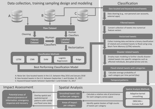
4.1. Data collection, training sampling design and modeling

In this study, we used three collections of Twitter data collected by Twitter’s Streaming API. The first dataset was collected using 11 hurricane-related keywords: ‘flood’, ‘irma’, ‘hurricaneirma’, ‘irmahurricane’, ‘irma2017’, ‘hurricane’, ‘damage’, ‘storm’, ‘rain’, ‘disaster’, ‘emergency’ in order to derive any tweet related to the disaster event. Although we did not use a statistical method to identify keywords that were mentioned statistically more during the disaster (Huang et al. 2018), we continuously updated our keywords using the most frequent hashtags throughout the disaster. We collected the second dataset using a spatial bounding box that covers the impact area of Irma in order to obtain geo-located tweets before, during and aftermath of the disaster. Both the first and second dataset include tweets from the time period beginning on 1 September 2017 and ending on 15 October 2017. Finally, we used a third dataset of randomly selected geo-located tweets from the Continental United States between the dates May 2017 and January 2018. We used the third dataset to incorporate noise in the training data collection. We picked random tweets from the third dataset to introduce the classification models noise to enhance the learning and prevent overfitting caused by the tweets from the study period. Combined database of the three datasets contained 756,913,748 tweets before processing and filtering. The keyword-based collection consisted of 64,266,068 tweets, in which 99% of these tweets have geo-location at least at the state level. About 64% of these tweets were retweets.

We included randomly selected geo-located tweets from the third dataset in the training sample without any filtering. On the other hand, we applied the following procedures to the first and the second dataset prior to the classification. We removed (1) retweets; (2) duplicated tweets by their tweet ids; (3) geo-located tweets from the second dataset that do not contain the predetermined set of keywords, which we derived from the list of keywords from the first dataset (Table 2); (4) tweets from non-personal user accounts such as weather apps and bots using the tweet source metadata. Table 3 lists the top sources for tweets, and whether we filtered them or not; (5) tweets that fall outside the time interval from 29 August 2017 to 16 October 2017; (6) tweets that do not contain information on geographic location, or tweets that are located outside the impact area of Hurricane Irma’s path. After the filtering, the data were reduced to 557,541 tweets that spanned a time period of one and a half months.

Table 2. Top 26 keyword counts in the raw dataset.

Keyword	Frequency	Hashtag	Frequency
rain	20,491,588	#rain	47,235	#hurricaneharvey	7883
hurricane	19,897,133	#irma	37,918	#disaster	5458
flood	13,489,668	#flood	20,821	irmahurricane	4298
storm	11,340,708	hurricaneirma	20,149	#irmahurricane	4180
irma	10,127,435	#emergency	19,972	#irma2017	2586
disaster	5,890,874	#storm	19,289	#damage	1932
emergency	5,514,237	#hurricaneirma	15,638	harveystorm	424
damage	5,179,521	hurricaneharvey	10,718	#harveystorm	416
#hurricane	56,389	irma2017	8727

Table 3. Filtering with the most common sources from Twitter metadata.

Source	% of tweets (and number)	Included
(Empty)	79.42% (601,179,529)	Yes
Twitter Web Client	6.79% (51,435,265)	Yes
Instagram	4.14% (31,389,138)	No
TweetMyJOBS	2.79% (21,186,456)	No
iPad	1.05% (7,991,578)	Yes
Foursquare	0.54% (4,130,888)	No
Tweetbot for iΟS	0.54% (4,092,581)	Yes
SafeTweet by TweetMyJOBS	0.43% (3,312,923)	No
Sandaysoft Cumulus	0.35% (2,715,771)	No
IFTTT	0.35% (2,674,435)	No
Twitter Lite	0.33% (2,521,005)	Yes
TweetDeck	0.29% (2,223,845)	Yes
dlvr.it	0.22% (1,711,766)	No
Cities	0.16% (1,238,873)	No
Facebook	0.12% (956,507)	Yes
Tweetbot for Mac	0.11% (895,958)	Yes
Hootsuite	0.10% (820,211)	No
Untappd	0.10% (813,913)	No

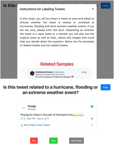
We designed a web-based interface to collect the training data for the binary classification of tweets: whether tweets are related to a hurricane, flooding or an extreme weather event (Figure 2(b)). We formed a team that consisted of the authors, undergraduate and graduate students for labeling the tweets. We trained our team based on the tasks using examples of both related and unrelated tweets. We considered any tweet whether it is informative or not, or it is about eye-witness information, or news story or warning, or critiques of the government and political discussions about the extreme weather events, flooding and the hurricanes as relevant. The web interface displays the tweet in its original form, and includes ‘Yes’ and ‘No’ buttons to answer the question. We included a ‘Not Sure’ button to let users skip the tweet if they are not sure about whether the tweet is relevant or not. The web interface starts with instructions on how to label the tweets with examples (Figure 2(a)). We specifically kept the question generic in contrast to being specific to Hurricane Irma, because the timespan of Irma overlapped with the other hurricanes such as Harvey, Maria and Jose, and some of the tweets in our dataset were related to those other hurricanes. This allowed us to generate a generic training dataset that can potentially be used for classification tasks for these multiple events. We collected approximately 20,000 labeled tweets with our team of human coders and the web-based interface.

Figure 2. (a) Instructions for the labeling task (b) Training data collection interface. ‘No’ and ‘Yes’ buttons to allow the user to label the presented tweet as ‘Related’ or ‘Unrelated’, or ‘Not Sure’ button is used to skip the tweet.

4.2. Binary classification of tweets

Using our training data, we performed classification experiments using Logistic Regression, Support Vector Machines (SVM), Convolutional Neural Networks (CNNs) and Long Short-Term Memory (LSTM) Networks. We describe each of these models and parameters in the following subsections.

4.2.1. Baseline classifier

We selected two different types of machine learning classifiers for comparison: (1) SVM with the Gaussian kernel to obtain a baseline classifier (2) a model with Principal Component Analysis (PCA) summarization step pipelined prior to the Gaussian SVM. We used the second model to evaluate the PCA’s effect on the classification task. We also evaluated results for several linear classifiers including Logistic Regression, Linear SVM and Ridge. These linear classifiers are expected to provide similar results due to the fixed linearity of the problem. The Gaussian SVMs use the radial basis function (RBF) as the similarity function while Linear SVMs use a linear similarity function. Thus, their difference in similarity functions makes them converge on different points. We evaluated alternative parameters and optimization settings for these models to improve the classification accuracy, and we report the experiment results for all five models in the Results section.

4.2.2. Convolutional Neural Networks (CNNs)

Artificial Neural Networks (ANNs) is a deep learning method that have been widely used for text classification tasks. ANNs allow learning the features of a phenomenon (e.g. words, combinations of words related to disasters) by progressively learning and evolving relevant characteristics from the learning material (training set) that they process. ANNs do not require any prior knowledge about the phenomenon. As a category of ANNs, Convolutional Neural Networks (CNNs) have been commonly used in text classification tasks. By eliminating the full connectivity of nodes in regular neural network layers, CNNs speed up the training process while sustaining the ability of creating non-linear models. Since CNNs were developed with the idea of the input as an image, CNNs utilize 3D neuron structures that have width, height and depth which commonly represent the width and height of an image as well as the color channels of the image respectively. While CNNs are mostly used in tasks that involve images, they are also capable of producing efficient and effective models in text classification (Burel, Saif, and Alani 2017).

Since our classification task is binary, we used the sigmoid (Equation (1)) function, that maps output values into [0, 1] set, as the final activation of the output layer. The output of the sigmoid function can then be converted into a class of 0 or 1 by using a threshold of 0.5. We used binary cross-entropy (Equation (2)) as the loss function in the CNN structure (Figure 1). Binary cross-entropy function measures the distance of a prediction made by the model from its actual value. The neural network is then updated in order to minimize this cost.

Sigmoid function, the activation function for neural network architectures(1) $\sigma \left(x\right)=\frac{1}{1+e^{-x}}.$(1)

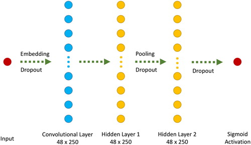
Binary cross-entropy function that is used as the loss function(2) $\mathcal{L}\left(y_i,{\hat{y}}_i\right)=-\frac{1}{N}\sum _{i=1}^N\left[y_i\log \left({\hat{y}}_i\right)+\left(1-y_i\right)\log \left(1-{\hat{y}}_i\right)\right].$(2) Figure 3 illustrates the architecture of our proposed CNN model which consists of a convolutional layer followed by two fully connected layers. Input is embedded before feeding it into the convolutional part. Dropouts and an additional pooling layer are applied to the outputs of some layers in order to prevent and control over-fitting.

Figure 3. Convolutional Neural Network Architecture.

4.2.3. Long Short-Term Memory (LSTM) Networks

Although CNNs may create robust classifiers (Burel et al. 2017; Nguyen et al. 2016), they are limited in memorizing features throughout the training process. Recurrent Neural Networks (RNNs) incorporate a pair of memory vectors that are trained at each step, which are then moved to next nodes or steps of training. For instance, in a word sequence, correlation of previous words with the intended output may affect the meaning of and possible inferences that can be made from latter words. This correlation of former words with the output should be carried on to the next nodes in order to capture the sequential nature of sentences. In a ‘vanilla’ RNN, the information that is being learned and kept in a feature vector (hidden state) changes irregularly. Due to the vanishing gradient problem, the weight of the neural network receives a vanishingly small proportion of the gradient of the loss which prohibits the learning process. As a result, the process of learning weights may be slow or even stop. Thus, a simple and modest RNN is not capable of remembering the features learned for long times. This mostly impacts the overall accuracy of text classification tasks.

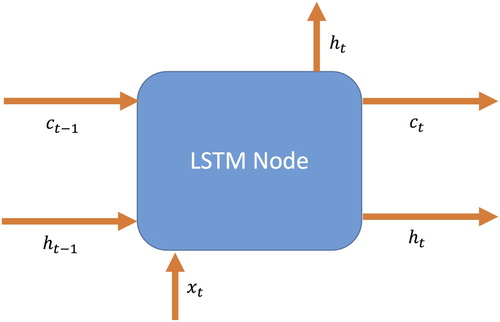
A Long Short-Term Memory Neural Network (Hochreiter and Schmidhuber 1997) extends the lifespan of the short-term memory to inherit more features into the deep neural network model. LSTMs and their variations are widely used in classification tasks that need longer memories, such as image classification (Byeon et al. 2015), text classification (Liu, Qiu, and Huang 2016) and time-series analysis (Xingjian et al. 2015). Figure 4 and the Equations (4)–(9) provide a brief summary of an LSTM node and mathematical background of an LSTM Node. The LSTM node is applied to tensors $x_t$ and $h_{t-1}$ in which $x_t$ represents the input, and $h_{t-1}$ represents the hidden state of the previous LSTM Node in the layer. Sigmoid function is represented by $\sigma (.)$ in Equation (1), and tanh(x) denotes hyperbolic tangent function (Equation (3)).

Figure 4. An LSTM Node and its connection formulations.

Hyperbolic tangent function(3) $\tanh \left(x\right)=\frac{e^x-e^{-x}}{e^x+e^{-x}}.$(3)

The weight matrices W and U transform input and hidden state vectors and forms $i_t$, $f_t$, $o_t$ and ${\tilde{c}}_t$ values, namely input gate (Equation (4)), forget gate (Equation (5)), output gate (Equation (6)) and cell update gate (Equation (7)) respectively. By virtue of these gates, LSTMs provide a forgetting mechanism to remove the features that are learned in previous nodes but are now obsolete. The ° operator represents an element-wise product, and the output of an LSTM Node is calculated by using these gates. While keeping the information in cell state (Equation (8)), LSTM nodes remember the information that will be used immediately in the hidden state (Equation (9)) which is similar to the hidden layer in RNNs. Finally, the hidden state and cell state are conveyed to the next LSTM Node, and the hidden state is conveyed to the next layer in the neural network architecture (Figure 5).

Figure 5. An LSTM layer and connections between LSTM nodes.

Input gate of an LSTM Node(4) $i_t=\sigma \left(W^{\left(i\right)}{x}_t+U^{\left(i\right)}{h}_{t-1}\right).$(4)

Forget gate of an LSTM Node(5) $f_t=\sigma \left(W^{\left(f\right)}{x}_t+U^{\left(f\right)}{h}_{t-1}\right).$(5)

Output gate of an LSTM Node(6) $o_t=\sigma \left(W^{\left(o\right)}{x}_t+U^{\left(o\right)}{h}_{t-1}\right).$(6) Cell update gate of an LSTM Node(7) ${\tilde{c}}_t=\tanh \left(W^{\left(c\right)}{x}_t+U^{\left(c\right)}{h}_{t-1}\right).$(7)

Cell state of an LSTM Node(8) $c_t=f_t\circ c_{t-1}+i_t\circ {\tilde{c}}_{t-1}.$(8)

Hidden state of an LSTM Node(9) $h_t=o_t\circ \tanh \left(c_t\right).$(9)

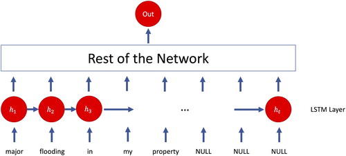
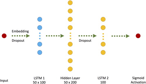
The deep neural network proposed here depends on LSTM networks along with other layers such as Embedding and Dropout layers (Figure 6). Similar to the proposed CNN model, we employed the sigmoid (Equation (1)) and binary cross-entropy (Equation (2)) functions in LSTM. We also evaluated the categorical cross-entropy function which did produce a better performance than the binary cross-entropy function. Thus, we do not report the results of the categorical cross-entropy function.

Figure 6. Proposed Long Short-term Memory (LSTM) Architecture.

4.2.4. Vectorization of the dataset

We vectorized the tweets to create an array that contains the tweet text, date and time stamp, and the binary label assigned by human classifiers during training dataset collection. An example tweet entry is illustrated below.$D_x=\left[\mathrm{T}\mathrm{w}\mathrm{e}\mathrm{e}\mathrm{t}\mathrm{T}\mathrm{e}\mathrm{x}\mathrm{t},\mathrm{D}\mathrm{a}\mathrm{t}\mathrm{e}\mathrm{a}\mathrm{n}\mathrm{d}\mathrm{T}\mathrm{i}\mathrm{m}\mathrm{e},\mathrm{L}\mathrm{a}\mathrm{b}\mathrm{e}\mathrm{l}\right],$ $D_x=["\mathrm{M}\mathrm{a}\mathrm{j}\mathrm{o}\mathrm{r}\mathrm{f}\mathrm{l}\mathrm{o}\mathrm{o}\mathrm{d}\mathrm{i}\mathrm{n}\mathrm{g}\mathrm{a}\mathrm{t}\mathrm{m}\mathrm{y}\mathrm{b}\mathrm{a}\mathrm{c}\mathrm{k}\mathrm{y}\mathrm{a}\mathrm{r}\mathrm{d}.\mathrm{h}\mathrm{t}\mathrm{t}\mathrm{p}\mathrm{s}://\mathrm{t}.\mathrm{c}\mathrm{o}/\mathrm{U}\mathrm{J}\mathrm{n}3\mathrm{s}","\mathrm{S}\mathrm{e}\mathrm{p}12,2017,22.13\mathrm{E}\mathrm{T}",1].$

To feed the information within the dataset into any kind of probabilistic classifier, the dataset needs to be represented by vectors. We performed pre-processing to filtering-out noisy tweets prior to converting the data into vectors. We first cleaned any kind of punctuation and URLs and transformed all characters to lower-case. We then split the text into a sequence of words in which sequences will be restructured as vectors. At the end of the pre-processing step, we derived a triple (tweet content, date and time stamp, and the label) of each tweet for the next step of tokenization.$D_x=\left[\left["\mathrm{m}\mathrm{a}\mathrm{j}\mathrm{o}\mathrm{r}","\mathrm{f}\mathrm{l}\mathrm{o}\mathrm{o}\mathrm{d}\mathrm{i}\mathrm{n}\mathrm{g}","\mathrm{a}\mathrm{t}","\mathrm{m}\mathrm{y}","\mathrm{b}\mathrm{a}\mathrm{c}\mathrm{k}\mathrm{y}\mathrm{a}\mathrm{r}\mathrm{d}"\right],"\mathrm{S}\mathrm{e}\mathrm{p}12,2017,22.13\mathrm{E}\mathrm{T}",1\right].$

After the sequencing step, we transformed each tweet to a vector using a tokenization centric approach, which is based on each word’s number of occurrences in the whole dataset. The more a word occurs in the dataset, the less it has an effect as a feature in the initialization of the network. We sorted the words in the dataset by their occurrence, and assigned indices starting from 1 to replace each word with an index. For instance, the word ‘flood’ has the highest frequency in the whole dataset, and therefore its index (replacement) is 1. Below is the transformed triple in which words were replaced by their integer indices.$D_x=\left[\left[515,252,34,17,4200\right],"\mathrm{S}\mathrm{e}\mathrm{p}12,2017,22.13ET",1\right].$

Since each tweet has different length, it’s crucial to pad the tweets to construct vectors with the same length and feed them into the neural network. We empirically tested different sizes for the vectorization process: 25, 30, 35, 40, 45, 50, 55 and 60. Classification test accuracy for the vectorized dataset with the length of 50 performed the best among all vector length options on the proposed LSTM architecture. While one column was used for the tweet post-date, the rest of the columns were used for the tweet tokens. Therefore, we chose 50 as the optimum number of vector size (49 word tokens + 1 date column) to derive semantics from a tweet. Following this assumption, we padded all vectors to generate a vector of zeros with a length of 49 words for each tweet.$D_x=\left[\left[0,\dots 0,515,252,34,17,4200\right],"\mathrm{S}\mathrm{e}\mathrm{p}12,2017,22.13\mathrm{E}\mathrm{T}",1\right].$

We incorporated the tweet post-date in tweet vectors in order to reveal the relationship between a tweet’s post-date and its relevancy with flooding and extreme weather events. Date-time tagging could be done for different temporal granularities such as by minute, hour, day or week. Although floods may occur suddenly, their impact, i.e. flood inundation often lasts days, weeks and in some instances longer time periods. Because our purpose was to capture the progression of the disaster over an extended period of time that include during and aftermath of Hurricane Irma, we chose day as the temporal resolution considering the occurrence and duration of the flood event and its impact in the aftermath of the hurricane. As a result, we mapped the dates between 29 August 2017 and 17 October 2017 on to an integer scale between 1 and 50, and we appended the integers into the feature vector. Finally, we derived a vector of length 50 for each tweet in the dataset, and the final vector of the example tweet is shown below:$D_x=\left[\left[0,\dots 0,515,252,34,17,4200\right],15,1\right].$

4.3. Thematic classification of disaster-relevant information

After classifying tweets related to flooding, hurricanes and extreme weather events, we employed an unsupervised topic modeling approach, Latent Dirichlet Allocation (LDA), to extract detailed information such as affected individuals, donations and support, caution and advice from tweet content. LDA is a Bayesian probabilistic model of documents that allows discovering a collection of latent topics defined as a multinomial distribution over words (Blei, Ng, and Jordan 2003). LDA assigns each document a mixture of topics.$P\left(Z|W,D\right)=\frac{W_{Z+\text{β}w}}{\mathrm{t}\mathrm{o}\mathrm{t}\mathrm{a}\mathrm{l}\mathrm{t}\mathrm{o}\mathrm{k}\mathrm{e}\mathrm{n}\mathrm{s}\mathrm{i}\mathrm{n}Z+\text{β}}\ast D_{Z+\propto }.$

For each topic Z, P (Z│W, D), the probability that word W came from topic Z, is calculated by multiplying the normalized frequency of W in Z with the number of other words in document D that already belong to Z. Hyper parameters such as β and βw are used to incorporate the probability that word W belongs to topic Z even if it is nowhere else associated with Z (Blei, Ng, and Jordan 2003). LDA iteratively goes through the collection of documents word by word and reassigns each word to a topic. After each iteration, the model becomes more consistent as topics with specific words and documents and reaches an equilibrium that is as consistent as the collection allows (Goldstone and Underwood 2012). The words become more common in topics when their frequencies are higher, and topics become more common in documents where they occur more often in documents. We used each tweet as a document to train the topic model. We first tokenized the tweets and converted them into lower case, and used stop words (e.g. commonly used words such as ‘the’, ‘of’, ‘am’) from 28 languages prior to training the model using the Mallet Toolkit (McCallum 2002). We did not use stemming, because stemming introduces noise to the results, and does not improve the interpretation of topic models (Schofield and Mimno 2016).

4.4. Spatially-adaptive kernel smoothing

Once each tweet is classified into a set of topics, one can calculate the average topical probabilities per unit area. For example, among 1000 disaster-related tweets in Sarasota County in Florida, one can calculate the average probability of a topic such as affected individuals, by simply dividing the sum of the probabilities of tweets that belong to affected individuals category to the total number of disaster-related tweets generated within the county. However, such an approach may suffer from the modifiable areal unit problem (MAUP) due to the mismatch between the impact of the disaster and the arbitrarily assigned administrative boundaries. Moreover, rates calculated for different geographic areas would have unequal reliability due to different population sizes, in our case, the total number of tweets, across the spatial units. This problem is exacerbated for small areas or in other words areas with low density of observations. Therefore, rates for areas with small population values become less reliable. To address the problem, spatially-adaptive kernel smoothing (Tiwari and Rushton 2005) can be applied to estimate a reliable density value of a feature by taking into account the nearby observations. Different from fixed-distance kernel smoothing, adaptive kernel smoothing defines a threshold for the denominator of the rate using the k-nearest observations (e.g. tweets or users). Using the number of users for determining the k-nearest neighbors help remove the user contribution bias, in which a few active users produce most of the content. However, in this study, we use number of tweets to determine the k-nearest neighbors because of two reasons. First, locational information is critical for the disaster context although it may be produced by only a few number of users. Second, large portion of tweets share the exact coordinates because the significant portion of tweets is place-tagged.

Definitions, the equations and steps of the adaptive kernel smoothing are defined below. In Step 1, the area is divided into a grid of 2.5 km resolution $\left(G\right)$, which covers Florida and the nearby affected areas of Hurricane Irma. There is a substantial amount of place-tagged tweets with the same coarse coordinates at city or neighborhood level. In Step 2, we aggregate the tweets that share the exact coordinates into distinct tweet locations prior to determining the k-nearest neighbors in order to prevent the potential bias. Therefore, we obtain a list of distinct tweet locations that include information on the total tweet count, the list of tweets and their assigned topical probabilities. We define k as the minimum number of distinct tweet locations to calculate a reliable estimate of the rate for each category of tweets. In Step 3, we employ a Sort-Tile-Recursive Tree algorithm to compute an index of the k-nearest distinct tweet locations for each grid cell in order to improve the computational efficiency. Once the neighborhood reaches the defined threshold k, we determine the list of tweets, T_i, bandwidth h (G_i, k), and the weights of distinct tweet locations for each grid cell in Step 3. K is the kernel function, and h is the bandwidth for smoothing. Kernel functions determine the weight of each observation within a kernel, and the choice of function often does not have substantial impact on the result. The most commonly used kernel functions are Uniform, Epanechnikov, Triangular and Gaussian. In this study, we employ the Gaussian kernel function to determine the weight of each tweet within the kernel of each grid cell. Given the list of tweets, the spatial weights and the probability of topics for each tweet, we compute a weighted average probability of each topic for each grid cell using the formula defined in Step 4.

Definitions:

• G: The study area defined by the total set of grid cells.

• G_i: Grid cell i. G_i ∈ G.

• k: Adaptive filter (neighborhood) threshold based on the total number of tweets.

• T_i: The list of tweets within the neighborhood of G_i.

• h (G_i, k): The bandwidth of the k-size Neighborhood of the grid cell G_i is defined as the smallest KNN (G_i, k) that has a total count of distinct tweet locations that is greater than or equal to k: ${\sum }_i^t\ge k.$

• K: Kernel function. Gaussian function is used in this study.

Steps:

1. Compute G, the grid of the study area given a resolution r. In this study r = 2.5 km is used.

2. Aggregate tweet statistics such as tweet count and topic probabilities of tweets for each distinct tweet location.

3. Construct a Sort-tile-recursive (STR) tree for finding the smallest k-nearest neighboring distinct tweet locations of G_i that meets the size constraint, k.

4. Compute T_i, h (G_i, k) and the weights of observations (tweets) for each grid-cell using the adaptive kernel estimation$f_h\left(P_z\left(G_i|\theta \right)\right)=\frac{1}{nh}\sum _{j=1}^{x\in T_i}K\left(\frac{x-x_j}{h}\right)p_z\left(t_i\right),$

where $P_z\left(G_i|\theta \right)$ is the weighted average probability of topic z given all the topical probabilities within the neighborhood of $G_i$, n is the total number of points (tweets), h is the bandwidth, x₁, x₂, … , x_n ∈ $T_i$ is a set of tweet locations within the neighborhood of $G_i$ , x is the location of estimation, and $p_z\left(t_j\right)$is the probability of topic z in tweet $t_j$.

4.5. Spatial clustering

In addition to using adaptive kernel smoothing to capture the relative prominence of each category of tweets across geographic space, we employ density-based spatial clustering with noise (DBSCAN) to identify areas where there is a high density of tweets for each category. Different from the smoothed surface of probability of each category, DBSCAN allows us to identify the areas in which the absolute density of tweets is greater than a defined threshold (Ester et al. 1996). DBSCAN requires two parameters: a search radius (Eps) and the minimum number of points within the search radius (MinPts). Unlike other clustering methods such as K-Means or K-Medoids, DBSCAN does not require the number of clusters as an input, and can capture clusters with arbitrary shapes. While a larger search radius (Eps) results in larger areas of spatial clusters, a smaller search radius results in smaller areas of interest. On the other hand, a larger MinPts results in more reliable detection of clusters, whereas a smaller MinPts results in many more clusters with increased noise and outlier points that are not assigned to any clusters. Finally, we calculate the smallest convex polygon that encloses each of the spatial clusters in order to identify areas in which high counts of tweets that belong to an information category (e.g. affected individuals) is spatially clustered. Ultimately, this allows us to identify areas where tweets from a particular information category are spatially clustered.

5. Results and evaluation

5.1. Experiments on binary classification

Using the vectorized version of the manually labeled dataset, we trained a series of binary classifiers. We included both related and unrelated data manually classified by human coders in our training set in order to increase the accuracy of models for predicting unrelated tweets. The dataset before any sampling consisted of 20,413 total tweets in which 7801 of them were manually classified as related and 12,612 of them were classified as unrelated.

We sub-sampled the labeled dataset to feed the model with the same amount of sequences for the binary classification, which consisted of 7801 related and 7801 unrelated tweets. Sub-sampled data were then split into the training and test sets in which the training set consisted 80% and the test set was 20%. After that, 12,481 training sequences and 3121 test sequences were used. Using the training set, we trained each disjoint model that include Logistic regression, SVM, CNN and LSTM models described in the methodology section with various parameter settings independently using the training set. Using the test set, we carried out a validation task for each model run. We optimized the model parameters to prevent overfitting and provide the best validation accuracy.

Table 4 illustrates the evaluation results of the models, which reveals that the LSTM networks and CNN-based models were significantly better than other conventional machine learning algorithms. Accuracy is measured as the fraction of true positive and true negatives over all of the classified tweets. While precision is the fraction of relevant tweets among all relevant tweets (i.e. true positives/(true positives + false positives)), recall is the fraction of relevant tweets over the total amount of tweets (true positives/(true positives + false negatives)). Finally, F1 score considers both the precision and recall given the formula:$\mathrm{F}1\mathrm{s}\mathrm{c}\mathrm{o}\mathrm{r}\mathrm{e}=2\ast \frac{\mathrm{p}\mathrm{r}\mathrm{e}\mathrm{c}\mathrm{i}\mathrm{s}\mathrm{i}\mathrm{o}\mathrm{n}\ast \mathrm{r}\mathrm{e}\mathrm{c}\mathrm{a}\mathrm{l}\mathrm{l}}{\mathrm{p}\mathrm{r}\mathrm{e}\mathrm{c}\mathrm{i}\mathrm{s}\mathrm{i}\mathrm{o}\mathrm{n}+\mathrm{r}\mathrm{e}\mathrm{c}\mathrm{a}\mathrm{l}\mathrm{l}}.$

Table 4. Accuracy, precision, recall and F1 scores for proposed classifier models.

	LSTM	CNN	CNN Kim (2014)	Logistic Regression	Gaussian SVM	Linear SVM	Gaussian SVM & PCA	Ridge
Accuracy	0.7478	0.7391	0.7250	0.5434	0.4985	0.4982	0.4915	0.5456
Precision	0.7541	0.7602	0.6999	0.5516	0.7608	0.5097	0.6250	0.5473
Recall	0.7488	0.7123	0.7826	0.5512	0.0220	0.3782	0.0031	0.6224
F1 Score	0.7514	0.7355	0.7389	0.5514	0.0428	0.4342	0.0062	0.5824

Overall, linear models produced better performance (F1 score) than the Gaussian RBF-based models. Although its difference from a random classifier is insignificant, Linear SVM produced an F1 Score of 0.4342, Gaussian SVMs produced high precision and low recall scores, which indicates a large number of false negative predictions. This inclination is reflected on the F1 Scores, as well. The Gaussian models can be chosen over the non-Gaussian SVM if high precision and low recall values are desired. By having an accuracy of approximately 55%, non-SVM Linear models revealed slightly better performance than a random classifier, however, these models were outperformed by the deep neural network classifiers.

We employed a variety of architectures utilizing both LSTM and CNN-based approaches in terms of the number of nodes and layers trained. We systematically evaluated the number of nodes in the input layer, which resulted in changes in padding values of the vectorization process for the training and test data. Additionally, we incorporated auxiliary neural network layers, such as pooling, dropout et cetera layers, into the proposed architectures in order to further optimize the model. In the training of the models that involved CNNs and LSTM networks, we obtained the best accuracy scores within the first few epochs by using the same batch size of 128 for both networks. To decrease the computation time, we accelerated the training processes of detailed neural networks by utilizing NVidia Tesla K80 GPUs. In addition to the models presented in the methodology section, we also report the results for the CNN model proposed by Kim (2014) that is trained on our training data and tested on our test set for further evaluation.

While both neural network architectures we proposed and the one we adopted from Kim (2014) performed similar, our LSTM-based network produced slightly a better performance than any of the CNN-based architectures in terms of both accuracy and F1 score. This uplift of the performance can be related to LSTMs’ ability in conveying previous information to the next nodes of the network. Although LSTMs take more time to train, time elapsed while predicting the class of a tweet did not change significantly. We should note that since our CNN model provided a better precision score of 0.7602 in return of lower recall score, one can choose the CNN over the LSTM network if the correctness of positive predictions has crucial importance. Similarly, the CNN architecture proposed by Kim (2014) resulted in a better recall score of 0.7826. Therefore, if the rate of actual positives is more important, model selection can be made in favor of this CNN model. We continued the rest of our analysis based on the outcome prediction of the LSTM model. We made this choice based on the overall performance of the model as well as the model’s ability to consider the sequential nature of text constructs. The LSTM based classifier predicted 378,474 related tweets (positives) and 179,050 unrelated tweets (negatives). We used this predicted set for thematic classification, and identifying temporal, spatio-temporal patterns of the thematic categories of disaster-related tweets.

5.2. Experiments and results of topic modeling

In this section, we present the experiments for selecting and interpreting the topic model parameters and results. In order to determine the optimum number of topics, we performed LDA using different number of topics such as 10, 20, 30, 40 and 50 topics with 2000 iterations. We evaluated the model outcomes to minimize the overlap of topics within each model, and the number of unique topics between topic models with the consecutive number of topics. In general, a topic model with a fewer number of topics generates combined topics, whereas a model with a larger number of topics results in less overlapping content (Newman et al. 2010). We used cosine similarity to measure the similarity of the models with different number of topics, and employed the following criteria to determine unique topics between two model outputs (Koylu 2018a): (1) The topic must have a probability threshold above 50% in order to eliminate noisy topics that only exist in a small number of documents. (2) The topic in the model with a larger number of topics should have a cosine similarity less than 20% with any of the topics of the model with a smaller number of k topics. Following these criteria, we compared the topic models with consecutive numbers such as 50–40, 40–30, 30–20 and 20–10 topics. The systematic evaluation of cosine similarity values both within and between models did not yield a clear result to justify the number of topics chosen for the model. However, the topic model with 30 topics produced much less within overlap than the 20-topic model, and this rate was smaller than the comparison of the 30-topic model to the 40-topic model. We manually observed the topics and individual tweets that were predominantly classified by each topic to determine the optimum number of topics. This evaluation also led us to the same number of topics, 30, as the optimum number that helped us determine the number of topics with minimal overlapping.

In order to diagnose the results of the topic model, we computed the measures of probability (P), document entropy (E) and corpus distance (CD) (Koylu 2018b). The probability of a topic represents how common a topic is across all tweets and is calculated by dividing the number of word tokens assigned to the topic by the sum of the token counts for all topics. If a topic has small probability, it means it exists only on a small number of tweets, and oftentimes there are not enough observations to examine the topic’s word distribution. On the other hand, if a topic has large probability, the topic is extremely frequent across many tweets. Topics with large probability of occurrence across documents are often considered as a collection of corpus specific stop-words. Besides the low and high probability topics, more interesting topics reside within the non-extreme values. We approximately set this range to be between 0.005 and 0.5. In addition to topic probability, document entropy represents the distribution characteristics of a topic across documents. For example, if entropy is high the topic is distributed evenly over documents (tweets), whereas if entropy is low the topic is concentrated on a smaller number of tweets. Finally, we use corpus distance which is calculated by Kullback–Leibler divergence. Corpus distance represents how far a topic is from the overall distribution of words in the corpus. A greater corpus distance means that the topic is more distinct as compared to the overall distribution of words, whereas a smaller distance means that the topic is more similar to the corpus distribution.

Table 5 illustrates the top 10 coherent topics, and the 2 outlier topics at the end of the table. The table includes both the words and metrics of each topic, and the words are ranked by their probability of occurrence from the highest to the lowest. One can infer the latent topic using the combination of the words that commonly co-occur. The first and the foremost important topic represents tweets about affected individuals and infrastructure that include personal updates, injuries, deaths, missing, found, or displaced people; and buildings, roads, utilities/services that are damaged, interrupted, restored or operational. The second topic represents the caution, warning and advice category, which includes guidance, tips, warnings issued or lifted, forecasting, and alerts about emergency response situations. The third topic represents donations and support which include needs, requests, or efforts for help, offers of money blood, shelter, supplies, and/or services by volunteers or professionals. The fourth topic represents the sympathy and emotional support category which includes thoughts, prayers, gratitude and sadness. The rest of the topics illustrates news, official reports, government response, critiques, and political discussions, missing pets, disrupted services, and self-reporting of hurricane preparedness of individuals. The last two topics, Topic 11 and Topic 12, in Table 5 are outlier topics. The eleventh topic is the topic with the highest probability that includes live-tweeting about the hurricane. These tweets are often not informative, and do not contain information about eye-witness accounts, or site-specific situations. The last topic in this table represents Spanish tweets about the hurricane.

Table 5. Twelve latent topics with words and diagnostics measures.

Topic	Words	P	E	CD
Affected individuals and infrastructure damage	hurricane, power, damage, storm, rain, house, wind, trees, water, winds, tree, flood, lost, lot, safe, update, flooding, Florida, hope, area	0.021	10.11	1.33
Caution, advice and warnings	Storm, rain, flood, surge, warning, tropical, hurricane, winds, wind, heavy, flooding, flash, Florida, area, watch, country, south, issued, tornado, water	0.015	9.72	1.68
Donations and volunteers	hurricane, relief, victims, donate, flood, Houston, money fund, disaster, support, Texas, efforts, donated, donations, benefit, hand, helping, Red, Cross, donating	0.019	10.04	1.73
Sympathy and emotional support	hurricane, safe, Florida, stay, storm, hope, prayers, family praying, path, friends, thoughts, coming, hoping, safety, irmahurricane, damage, south, heart	0.030	10.45	1.30
News and official reports	hurricane, Florida, shoot, police, looters, Miami, guns, Richard, island, Branson, storm, news, video, looting, caught, warn, sign, private, foot, rescue	0.050	8.76	2.40
Government response, critiques and political discussions	hurricane, relief, disaster, victims, aid, Trump, tax, FEMA, Florida, Texas, house, recovery, voted, emergency, efforts, response, funding, money, flood, cuts	0.011	9.46	1.85
Government response, critiques and political discussions	hurricane, disaster, natural, damage, Trump, storm, flood, victims, disasters, lives, relief, country, Texas, North, Korea, America, Houston, worst, season, president	0.021	10.12	1.31
Affected individuals and missing pets	hurricane, flood, victims, pets, animals, dogs, left, dog, rescue, Houston, abandoned, cats, Texas, key, owners, storm, west, Florida, family, shelter	0.009	9.25	2.07
Disrupted service and tips for recovery	hurricane, power, storm, service, phone, internet, free, Florida, app, wifi, data, lost, work, cell, watch, lose, emergency, week, working, wait	0.010	9.40	1.80
Preparedness	hurricane, water, food, snacks, eat, gas, easting, supplies, prep, ready, storm, house, buy, power, coming, store, party, beer, open, bought	0.019	10.01	1.60
Chatting about the hurricane	hurricane, coming, Florida, y’all, storm, house, season, hope, scared, leave, category, party, bout, mom, jose, hits, making, work, Miami, cat	0.065	11.23	0.94
Spanish tweets	huracan, Florida, Cuba, paso, vea, Miami, categoria, caribe, video, vivo, fotos, llegada, isla, minute, mertos, danos, mar, imagenes, vientos, cayos	0.008	9.29	2.99

Notes: P: Probability, E: Entropy, CD: Corpus Distance.

5.3. Temporal, spatial and spatio-temporal patterns

Figure 7 illustrates the temporal probability distribution of the 10 coherent topics shown in Table 5. The probability of donations and support, and sympathy and prayers categories increased prior to the disaster, decreased during the disaster, and increased after Hurricane Irma dissipated. As an exception, both of these two categories were high on September 3, which coincided with the immediate aftermath of Hurricane Harvey that hit Texas and the surrounding areas prior to Hurricane Irma. Similarly, sympathy and prayers increased prior to the disaster, decreased during the disaster, and started to increase after Hurricane Irma dissipated. Advice, warning and alerts also had a similar increasing trend before the disaster, and in the aftermath of the disaster’s impact in Florida. Government critiques also had an increasing trend after the hurricane dissipated. Another notably interesting pattern is that tweets about affected individuals started to increase right after September 6 when Irma reached its peak with wind speed and made the first landfall in Florida on September 10. We provide a random sample of original tweet content with their assigned topics for affected individuals and infrastructure category in Table 6, and for all other categories in Table 7 in the Appendix section.

Figure 7. Temporal distribution of top 10 coherent categories of disaster-related tweets.

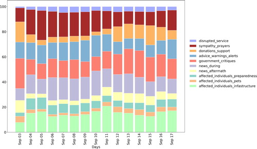
Table 6. Sample of tweets for each category of information.

C	EST 2017	Tweet	P
Affected individuals and preparedness	Tue Sep 05 19:21	Everybody stocking up for the hurricane	0.83
	Wed Sep 06 10:35	Prepping for Hurricane Irma but I’m never too busy to get down on some delicious.	0.68
	Wed Sep 06 11:18	It’s hard to prepare for a storm when there are no supplies to buy and no gas to leave I’m all good but friends not so much!!	0.60
	Wed Sep 06 21:18	Im gonna eat all the hurricane food before the actual hurricane	0.92
	Thu Sep 07 20:00	Super disappointed to see my local gas station in Clermont; Florida selling water for $22 per case during hurricane prep.	0.97
	Sat Sep 09 18:56	I’d try to be a bit more helpful; but still in the middle of hurricane prep atm	0.31
	Sat Sep 09 20:28	Just spent over $40 on gas; thanks Irma	0.83
	Sun Sep 10 14:50	Well I Just Ate My Last Bag Of Hot Cheetos And Them Was My Hurricane Snacks	0.94
	Sun Sep 10 19:33	I know for a fact everyone is bored out of their mind and has eaten a good 50% of their hurricane food	0.92
	Mon Sep 25 21:33	Why are people so dumb. Why does nobody keep a 3 month emergency kit? 3 months food and emergency supplies; put it in a big bin. Done.	0.83
Affected individuals and infrastructure	Thu Sep 07 12:40	I just realized I might not have power for the comeback because of Hurricane Irma!!	0.19
	Sun Sep 10 10:45	Hunkered down in a block house w/hurricane shutters. 4 people; 2 dogs; 2 cats; and 4 fish. Come at us	0.48
	Mon Sep 11 15:56	I ain’t think irma hit this bad but there’s trees in the streets and all	0.83
	Mon Sep 11 17:51	Hurricane Irma left a mark on my yard in Grayson …	0.92
	Tue Sep 12 11:56	Savannah may have some cleaning up to do. Lots of folks in S. Georgia are out of power due to Irma	0.94
	Tue Sep 12 12:23	Too bad Irma took my power	0.42
	Wed Sep 13 21:32	People driving ruthlessly during Irma power outage. Crossing over double line; not looking before turning; speeding in parking lots.	0.96
	Fri Sep 15 15:35	I’m very sorry we are still recuperating from hurricane Irma and we still have no power. Very sorry that we will not be opened this weekend.	0.74
	Fri Sep 15 17:27	From inside the gazebo! Hurricane Irma took out the garden … we need chainsaws and bucket trucks!!!	0.62
	Mon Oct 09 17:36	I live in FL I lost power in Irma don’t recall relying on fed’s to get our power. PR needs to do something	0.48

Notes: C (Category), P (Probability).

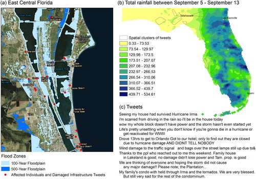
In this article, we only report the semantic, spatial and spatio-temporal characteristics of affected individuals and damaged infrastructure category, which we will refer to this category as affected individuals in the rest of the article. In order to calculate the smoothed ratio of affected individual tweets, we used k = 10 as the minimum number of distinct tweet locations. In addition to the smoothed rate that illustrates the prominence of each category relative to all categories, we also extracted areas where there is a high density of tweets that belong to each category using the DBSCAN algorithm. We experimented with a range of Eps values: 10, 20, 30, 40, and 50 km; and a range of MinPts such as 5, 10, 15 and 20 distinct tweet locations. Higher Eps and lower MinPts values resulted in clusters that are quite large, while lower Eps and higher MinPts values resulted in many clusters, and outlier tweet locations that were not classified part of the cluster. Values of 30 km for Eps and 10 distinct tweet locations for MinPts produced 32 clusters which were consistent with the impacted areas of the hurricane. Also, this combination minimized the number of outliers in the clustering process. Figure 8 illustrates the ratio of affected individual tweets to tweets from all categories (i.e. the results of Section 4.4), the areas where there is a high density of tweets for affected individual tweets (i.e. the results of Section 4.5) as well as the temporal histogram of frequency for this category. There were a total of 14,724 tweets that had at least 50% probability for belonging to the affected individuals and infrastructure category. Because of the high presence of place-tagged tweets, the number of distinct tweet locations was 7709, which corresponds to approximately 2% of all tweets in the study area. Among these tweets, 501 tweets were place-tagged at the state level (Florida), therefore, these tweets were excluded prior to computing the smoothed rate.

Figure 8. Spatial and temporal distribution of tweets about affected individuals and infrastructure.

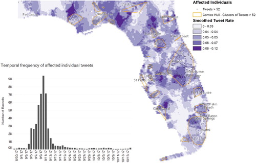
In Figure 8, the temporal frequency of tweets about affected individuals was higher between September 5 and September 13, when the storm made the landfall, and areas in Florida were inundated. The smoothed rate surface illustrates the relative prominence of affected individual and infrastructure tweets, while the convex hulls of tweet clusters helps distinguish the areas where there are higher count of tweets from the selected category. This figure confirms some of the highly damaged areas and areas with disrupted services such as the urban areas of Tallahassee, Jacksonville, Orlando and Tampa, Florida Keys, and the coastal areas in the east such as Palm Bay and Rockledge.

In order to better assess the potential damage and affected individuals, we overlayed the tweets and potential impact areas with flood zone (Figure 9(a)) and rainfall data (Figure 9(b)). The total rainfall is spatially correlated with clusters of affected individual tweets in some impact areas such as the north-east of Cape Coral, the impact zones around Jacksonville, Orland and Port St. Lucie, while spatial clusters of affected individual tweets do not correlate with rainfall in most other areas (Figure 9(b)). This could potentially be explained by the damage from other weather events such as high winds and tornadoes. In Figure 9(a), we illustrate the area of East Central Florida, in which five tornadoes caused significant damage during the hurricane.

Figure 9. Overlaying of tweets with total rain in inches and flood zones between September 5 and September 12.

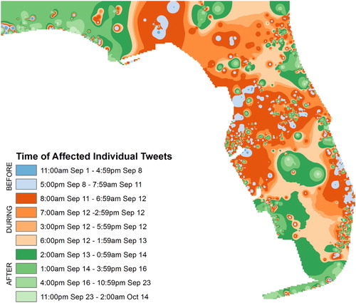
In order to reveal the temporal progression of the affected individual tweets, we interpolated the date and time of tweets using inverse-distance weighting (IDW) interpolation (Figure 10). Three color hues are used to illustrate the temporal progression of affected individual tweets for the study area before (blue), during (orange) and after (green) Irma. An interesting finding of this map is that there are a large number of areas with large variation (small patches of different color hues) in terms of the time of tweets, as people continued to tweet before, during and after the hurricane. On the other hand, green areas illustrate highly impacted zones which required greater intensity of response and recovery efforts in the aftermath of the hurricane. People in these areas did not tweet as much before or during the storm, which could be attributed to the potential loss of power and phone services.

Figure 10. Temporal progression of affected individuals and infrastructure tweets by area. On average, Blue areas tweeted before, orange areas tweeted during, and green areas tweeted after Hurricane Irma.

6. Discussion and conclusion

Knowing what information is available through social media helps emergency responders, humanitarian organizations, governments and utility companies prepare and respond to disasters by effective allocation of their limited resources. Identifying disaster-related social media posts have recently been the focus of many studies that aim to understand the extent and magnitude of damage, and improve the ways we identify affected individuals, develop situational awareness and coordinate recovery efforts. Our study contributes to these studies by introducing a methodology that integrates deep learning, natural language processing and spatio-temporal analysis to identify content, whereabouts and temporal context of disaster-related social media posts.

In order to define our specific contributions to the studies that focus on the classification of crisis-related information from social media data, here we compare and contrast our methodology and results with the previous work done by Burel, Saif, and Alani (2017), Nguyen et al. (2016), Olteanu, Vieweg, and Castillo (2015) and others. First, unlike the previous work which focuses on identifying events and targeting immediate response to disasters, our overall objective is rather holistic to capture any useful information that may be related to the progression of a hurricane including the preparedness, response and recovery stages. Using a two-step classification approach, we identified relevant tweets to a hurricane with specific categories of information which have different target audience such as emergency responders, rescue missions and utility companies, animal control and shelters; government organizations and non-profit institutions that organize recovery and relief efforts; and local governments and FEMA for building and enhancing situational awareness. Second, we collapsed the three categories: related and informative, related but not informative, and not related introduced by Olteanu, Vieweg, and Castillo (2015) into a binary category of related and not related. We used the binary classification for two reasons. Human classifiers have shown significant variation in the labeling task especially when the task is complex and ambiguous (Nguyen et al. 2016). Moreover, we argue that labeling tweets as informative and not informative by simply evaluating the text of the tweet may often be inadequate without examining the content, time and location of tweets.

Burel et al. (2017) employed a three-tiered classification system for extracting (1) Crisis vs non-crisis (2) Type of crisis (flood, fire, etc.) (3) Type of information (affected individuals, donations, etc.). There are many differences between our study and Burel and colleagues. Data used by Burel and colleagues consist of 28,000 tweets. In our study, our training data consist of approximately 20,000 labeled data, and we classified 557,524 tweets using our training set and the classification methods. We chose the LSTM model for the binary classification task because (1) LSTMs are conceptually a better fit for the text classification task, since LSTMs consider the ordering of words and the whole text structure by using long-term semantic word and feature dependencies. (2) While both neural network architectures performed similarly, LSTMs produced slightly a better performance than CNN-based architecture in terms of both accuracy and F1 score. While Burel achieves high performance (F1 scores) for detecting crisis and non-crisis situations and event types, the performance of their model for identifying fine-grained event information such as affected individuals, damaged infrastructure is low (60%). Also, their classification model cannot handle multiple labels where a tweet can belong to two categories such as affected individual and advice and caution. Similarly, Nguyen and colleagues reported lower classification performance for information types, and they attributed the lower performance to the conflicting annotation done by online workers and volunteers. In contrast to these studies, we employed LDA as an unsupervised approach to extract the fine-grained details of information about the crisis situation, which also allowed us to classify each tweet with multiple labels such as affected individual and caution and advice.

Another unique aspect of our study is that we obtained information before, during and aftermath of the disaster as compared to retrospective studies which often lack the data during the first few hours of the event. Since the hazard type is a hurricane we were able to start collecting the data using a set of keywords related to the forecasted hurricane as well as geo-located tweets using the study area. We continued to collect the data a month after Hurricane Irma was formed, and we continuously updated the keywords based on the most common hashtags used throughout the hurricane. For future studies, we would like to compare the impact of the hurricanes Harvey, Irma and Maria.

The methodology introduced in this article has great potential to be used during a disaster for real-time identification of damage and emergency information, and making informed decisions by assessing the situation in impacted areas. Due to the limited space, we did not provide an in-depth analysis of the site-specific information we gained through analysis, however, we plan to conduct future work to evaluate damage, extract site and individual-specific information from various categories of disaster-relevant tweets.

Disclosure statement

No potential conflict of interest was reported by the authors.

ORCID

Muhammed Ali Sit http://orcid.org/0000-0002-2707-6692

Caglar Koylu http://orcid.org/0000-0001-6619-6366

Ibrahim Demir http://orcid.org/0000-0002-0461-1242

References

- Acar, A., and Y. Muraki. 2011. “Twitter for Crisis Communication: Lessons Learned from Japan’s Tsunami Disaster.” International Journal of Web Based Communities 7 (3): 392–402. doi: 10.1504/IJWBC.2011.041206
- Blei, D. M., A. Y. Ng, and M. I. Jordan. 2003. “Latent Dirichlet Allocation.” The Journal of Machine Learning Research 3: 993–1022.
- Burel, G., H. Saif, and H. Alani. 2017. “Semantic Wide and Deep Learning for Detecting Crisis-information Categories on Social Media.” Paper presented at the International Semantic Web Conference.
- Burel, G., H. Saif, M. Fernandez, and H. Alani. 2017. “On Semantics and Deep Learning for Event Detection in Crisis Situations.” In Workshop on Semantic Deep Learning (SemDeep), at ESWC 2017, 29 May 2017, Portoroz, Slovenia.
- Byeon, W., T. M. Breuel, F. Raue, and M. Liwicki. 2015. “Scene Labeling with Lstm Recurrent Neural Networks.” Paper presented at the Proceedings of the IEEE Conference on Computer Vision and Pattern Recognition.
- Caragea, C., N. McNeese, A. Jaiswal, G. Traylor, H.-W. Kim, P. Mitra, and B. J. Jansen. 2011. “Classifying Text Messages for the Haiti Earthquake.” Paper presented at the Proceedings of the 8th International Conference on Information Systems for Crisis Response and Management (ISCRAM2011).
- Caragea, C., A. Silvescu, and A. H. Tapia. 2016. “Identifying Informative Messages in Disaster Events Using Convolutional Neural Networks.” Paper presented at the International Conference on Information Systems for Crisis Response and Management.
- Cervone, G., E. Sava, Q. Huang, E. Schnebele, J. Harrison, and N. Waters. 2016. “Using Twitter for Tasking Remote-sensing Data Collection and Damage Assessment: 2013 Boulder Flood Case Study.” International Journal of Remote Sensing 37 (1): 100–124. doi: 10.1080/01431161.2015.1117684
- De Albuquerque, J. P., B. Herfort, A. Brenning, and A. Zipf. 2015. “A Geographic Approach for Combining Social Media and Authoritative Data Towards Identifying Useful Information for Disaster Management.” International Journal of Geographical Information Science 29 (4): 667–689. doi: 10.1080/13658816.2014.996567
- De Choudhury, M., N. Diakopoulos, and M. Naaman. 2012. “Unfolding the Event Landscape on Twitter: Classification and Exploration of User Categories.” Paper presented at the Proceedings of the ACM 2012 conference on Computer Supported Cooperative Work.
- Demir, I., H. Conover, W. F. Krajewski, B.-C. Seo, R. Goska, Y. He, and W. Petersen. 2015. “Data-enabled Field Experiment Planning, Management, and Research Using Cyberinfrastructure.” Journal of Hydrometeorology 16 (3): 1155–1170. doi: 10.1175/JHM-D-14-0163.1
- Doggett, E. V., and A. Cantarero. 2016. “Identifying Eyewitness News-worthy Events on Twitter.” Paper presented at the Conference on Empirical Methods in Natural Language Processing.
- Ester, M., H.-P. Kriegel, J. Sander, and X. Xu. 1996. “A Density-based Algorithm for Discovering Clusters in Large Spatial Databases with Noise.” Paper presented at the Knowledge Discovery and Data Mining (KDD), Portland, OR.
- Fang, R., A. Nourbakhsh, X. Liu, S. Shah, and Q. Li. 2016. “Witness Identification in Twitter.” Paper presented at the Proceedings of the Fourth International Workshop on Natural Language Processing for Social Media, Austin, TX, USA.
- Feng, Y., and M. Sester. 2018. “Extraction of Pluvial Flood Relevant Volunteered Geographic Information (VGI) by Deep Learning from User Generated Texts and Photos.” ISPRS International Journal of Geo-Information 7 (2): 39. doi: 10.3390/ijgi7020039
- Goldstone, A., and T. Underwood. 2012. “What Can Topic Models of PMLA Teach us about the History of Literary Scholarship.” Journal of Digital Humanities 2 (1): 39–48.
- Hagen, L., T. Keller, S. Neely, N. DePaula, and C. Robert-Cooperman. 2017. “Crisis Communications in the Age of Social Media: A Network Analysis of Zika-related Tweets.” Social Science Computer Review 36 (5): 523–541. doi: 10.1177/0894439317721985
- Herfort, B., J. P. de Albuquerque, S.-J. Schelhorn, and A. Zipf. 2014. “Exploring the Geographical Relations Between Social Media and Flood Phenomena to Improve Situational Awareness.” In Connecting a Digital Europe Through Location and Place, edited by Joaquin Huerta, Sven Schade, and Carlos Granell, 55–71. Heidelberg: Springer.
- Hochreiter, S., and J. Schmidhuber. 1997. “Long Short-term Memory.” Neural Computation 9 (8): 1735–1780. doi: 10.1162/neco.1997.9.8.1735
- Huang, Q., G. Cervone, and G. Zhang. 2017. “A Cloud-enabled Automatic Disaster Analysis System of Multi-sourced Data Streams: An Example Synthesizing Social Media, Remote Sensing and Wikipedia Data.” Computers, Environment and Urban Systems 66: 23–37. doi: 10.1016/j.compenvurbsys.2017.06.004
- Huang, X., C. Wang, Z. Li, and H. Ning. 2018. “A Visual–Textual Fused Approach to Automated Tagging of Flood-related Tweets During a Flood Event.” International Journal of Digital Earth, 1–17. doi:10.1080/17538947.2018.1523956.
- Imran, M., S. Elbassuoni, C. Castillo, F. Diaz, and P. Meier. 2013. “Extracting Information Nuggets from Disaster-related Messages in Social Media.” Paper presented at the ISCRAM.
- Kanhabua, N., and W. Nejdl. 2013. “Understanding the Diversity of Tweets in the Time of Outbreaks.” Paper presented at the Proceedings of the 22nd International Conference on World Wide Web.
- Kim, Y. 2014. “Convolutional Neural Networks for Sentence Classification.” arXiv preprint arXiv:1408.5882.
- Kongthon, A., C. Haruechaiyasak, J. Pailai, and S. Kongyoung. 2012. “The Role of Twitter During a Natural Disaster: Case Study of 2011 Thai Flood.” Paper presented at the Technology Management for Emerging Technologies (PICMET), 2012 Proceedings of PICMET’12.
- Koylu, C. 2018a. “Modeling and Visualizing Semantic and Spatio-temporal Evolution of Topics in Interpersonal Communication on Twitter.” International Journal of Geographical Information Science: 1–28. doi:10.1080/13658816.2018.1458987.
- Koylu, C. 2018b. “Uncovering Geo-social Semantics from the Twitter Mention Network: An Integrated Approach Using Spatial Network Smoothing and Topic Modeling.” In Human Dynamics Research in Smart and Connected Communities, edited by S.-L. Shaw, and D. Sui, 163–179. Cham: Springer International.
- Krajewski, W. F., D. Ceynar, I. Demir, R. Goska, A. Kruger, C. Langel, and B.-C. Seo. 2017. “Real-time Flood Forecasting and Information System for the State of Iowa.” Bulletin of the American Meteorological Society 98 (3): 539–554. doi: 10.1175/BAMS-D-15-00243.1
- Kryvasheyeu, Y., H. Chen, N. Obradovich, E. Moro, P. Van Hentenryck, J. Fowler, and M. Cebrian. 2016. “Rapid Assessment of Disaster Damage Using Social Media Activity.” Science Advances 2 (3): e1500779. doi: 10.1126/sciadv.1500779
- Kumar, S., F. Morstatter, R. Zafarani, and H. Liu. 2013. “Whom Should I Follow?: Identifying Relevant Users During Crises.” Paper presented at the Proceedings of the 24th ACM Conference on Hypertext and Social Media.
- Kwon, H. Y., and Y. O. Kang. 2016. “Risk Analysis and Visualization for Detecting Signs of Flood Disaster in Twitter.” Spatial Information Research 24 (2): 127–139. doi:10.1007/s41324-016-0014-1.
- Lachlan, K. A., P. R. Spence, X. Lin, K. Najarian, and M. Del Greco. 2016. “Social Media and Crisis Management: CERC, Search Strategies, and Twitter Content.” Computers in Human Behavior 54: 647–652. doi: 10.1016/j.chb.2015.05.027
- Li, Z., C. Wang, C. T. Emrich, and D. Guo. 2018. “A Novel Approach to Leveraging Social Media for Rapid Flood Mapping: A Case Study of the 2015 South Carolina Floods.” Cartography and Geographic Information Science 45 (2): 97–110. doi:10.1080/15230406.2016.1271356.
- Liu, S. B., L. Palen, J. Sutton, A. Hughes, and S. Vieweg. 2008. “In Search of the Bigger Picture: The Emergent Role of On-line Photo Sharing in Times of Disaster.” Paper presented at the Proceedings of the Information Systems for Crisis Response and Management Conference (ISCRAM).
- Liu, P., X. Qiu, and X. Huang. 2016. “Recurrent Neural Network for Text Classification with Multi-task Learning.” arXiv preprint arXiv:1605.05101.
- Maantay, J., A. Maroko, and G. Culp. 2010. “Using Geographic Information Science to Estimate Vulnerable Urban Populations for Flood Hazard and Risk Assessment in New York City.” In Geospatial Techniques in Urban Hazard and Disaster Analysis. Vol. 2., edited by P. S. Showalter and Y. Lu, 71–97. Dordrecht: Springer.
- McCallum, A. K. 2002. MALLET: A Machine Learning for Language Toolkit [online]. Available from: http://mallet.cs.umass.edu [Accessed 28 Dec 2018]
- Monroy-Hernández, A., E. Kiciman, M. De Choudhury, and S. Counts. 2013. “The New War Correspondents: The Rise of Civic Media Curation in Urban Warfare.” Paper presented at the Proceedings of the 2013 Conference on Computer Supported Cooperative Work.
- Munro, R., and C. D. Manning. 2012. “Short Message Communications: Users, Topics, and In-language Processing.” Paper presented at the Proceedings of the 2nd ACM Symposium on Computing for Development.
- Nelson, L. D., P. R. Spence, and K. A. Lachlan. 2009. “Learning from the Media in the Aftermath of a Crisis: Findings from the Minneapolis Bridge Collapse.” Electronic News 3 (4): 176–192. doi: 10.1080/19312430903300046
- Newman, D., J. H. Lau, K. Grieser, and T. Baldwin. 2010. “Automatic Evaluation of Topic Coherence.” Paper presented at the Human Language Technologies: The 2010 Annual Conference of the North American Chapter of the Association for Computational Linguistics.
- Nguyen, D. T., S. Joty, M. Imran, H. Sajjad, and P. Mitra. 2016. “Applications of Online Deep Learning for Crisis Response Using Social Media Information.” arXiv preprint arXiv:1610.01030.
- Olteanu, A., C. Castillo, F. Diaz, and S. Vieweg. 2014. “CrisisLex: A Lexicon for Collecting and Filtering Microblogged Communications in Crises.” Paper presented at the ICWSM.
- Olteanu, A., S. Vieweg, and C. Castillo. 2015. “What to Expect When the Unexpected Happens: Social Media Communications Across Crises.” Paper presented at the Proceedings of the 18th ACM Conference on Computer Supported Cooperative Work & Social Computing.
- Pekar, V., J. Binner, H. Najafi, and C. Hale. 2016. “Selecting Classification Features for Detection of Mass Emergency Events on Social Media.” Paper presented at the Proceedings of the International Conference on Security and Management (SAM).
- Restrepo-Estrada, C., S. C. de Andrade, N. Abe, M. C. Fava, E. M. Mendiondo, and J. P. de Albuquerque. 2018. “Geo-social Media as a Proxy for Hydrometeorological Data for Streamflow Estimation and to Improve Flood Monitoring.” Computers & Geosciences 111: 148–158. doi: 10.1016/j.cageo.2017.10.010
- Schnebele, E. 2013. “Improving Remote Sensing Flood Assessment Using Volunteered Geographical Data.” Natural Hazards and Earth System Sciences 13 (3): 669. doi: 10.5194/nhess-13-669-2013
- Schofield, A., and D. Mimno. 2016. “Comparing Apples to Apple: The Effects of Stemmers on Topic Models.” Transactions of the Association for Computational Linguistics 4: 287–300. doi: 10.1162/tacl_a_00099
- Smith, L., Q. Liang, P. James, and W. Lin. 2015. “Assessing the Utility of Social Media as a Data Source for Flood Risk Management Using a Real-time Modelling Framework.” Journal of Flood Risk Management 10 (3): 370–380. doi: 10.1111/jfr3.12154
- Spielhofer, T., R. Greenlaw, D. Markham, and A. Hahne. 2016. “Data Mining Twitter During the UK Floods: Investigating the Potential Use of Social Media in Emergency Management.” Paper presented at the Information and Communication Technologies for Disaster Management (ICT-DM), 2016 3rd International Conference on.
- Stefanidis, A., A. Cotnoir, A. Croitoru, A. Crooks, M. Rice, and J. Radzikowski. 2013. “Demarcating New Boundaries: Mapping Virtual Polycentric Communities Through Social Media Content.” Cartography and Geographic Information Science 40 (2): 116–129. doi:10.1080/15230406.2013.776211.
- Tiwari, C., and G. Rushton. 2005. “Using Spatially Adaptive Filters to Map Late Stage Colorectal Cancer Incidence in Iowa.” In Developments in Spatial Data Handling, edited by F. Peter Fisher, 665–676. Berlin: Springer.
- Vieweg, S., A. L. Hughes, K. Starbird, and L. Palen. 2010. “Microblogging During Two Natural Hazards Events: What Twitter May Contribute to Situational Awareness.” Paper presented at the Proceedings of the SIGCHI Conference on Human Factors in Computing Systems.
- Xingjian, S., Z. Chen, H. Wang, D.-Y. Yeung, W.-K. Wong, and W.-C. Woo. 2015. “Convolutional LSTM Network: A Machine Learning Approach for Precipitation Nowcasting.” Paper presented at the Advances in Neural Information Processing Systems.
- Zhang, Y., C. Szabo, and Q. Z. Sheng. 2016. “Improving Object and Event Monitoring on Twitter Through Lexical Analysis and User Profiling.” Paper presented at the International Conference on Web Information Systems Engineering.