Defining hydroclimatic regions using daily rainfall characteristics in the southern Appalachian Mountains

ABSTRACT

This paper addresses warm season hydroclimatic variability in the southern Appalachian region of the southeastern U.S., where precipitation can vary as much as 127 mm or more, with maximum seasonal totals exceeding 736 mm in extreme cases. Despite the occurrence of droughts, floods, and their socioecological impacts, hydroclimate variability is still poorly understood. This study characterizes the regional scale variations in the hydroclimate by examining the daily distribution of precipitation patterns in different topographic environments. Parameter-elevation relationships on independent slopes model (PRISM) gridded precipitation estimates are used to identify the location and frequency of different types of rainfall events. Several types of clustering algorithms are used as a regionalization approach to define areas where the precipitation regime exhibits similarities in its frequency of occurrence. The results are compared with internal validation statistics and a visualization is used to assess how well the resulting hydroclimatic regions align with different topographic environments. This study reveals the intricate spatial footprint of dry and wet regimes and demonstrates how clustering applications can be used with gridded climate data to determine where extremes are most likely to develop across mountain catchments.

KEYWORDS:

• Hydroclimatology
• precipitation
• cluster analysis
• data mining
• visualization

1. Introduction

The hydroclimatology of mountain regions influences the quality and quantity of regional water resources yet is poorly understood in the context of climate variability and change. General circulation models project an increase in hydroclimatic variability during the next century throughout many mid-latitude regions (Christensen et al. 2013), but the degree of change with regard to the timing and pattern of precipitation in mountain regions is complex to model and therefore difficult to predict. An improved knowledge of the hydroclimatology of mountain regions is needed to understand how the existing precipitation patterns may be changing in a changing climate.

The hydroclimatology of mountain regions is complex for several reasons. First, the spatial patterns of precipitation in mountains are not well documented or understood, primarily because they are difficult to observe (Barry 2008). Weather stations are typically confined to valley locations, which limits observations from higher terrain or in remote areas. Second, precipitation patterns exhibit enormous complexity across mountain catchments due to orographic enhancement (Barros and Lettenmaier 1993; Sinclair et al. 1997; Nykanen and Harris 2003; Frame and Markowski 2006). For example, prominent ridgelines, concave areas, and broad, high plateaus increase the frequency of precipitation events, while decreased precipitation is observed in leeward areas (Lin et al. 2001). Finally, atmospheric circulation, including the phase of various teleconnections (Kahya and Dracup 1993; Katz, Parlange, and Tebaldi 2003), as well as the direction of low-level flow and positioning of features in the middle troposphere, dictate the extent and intensity of rainfall over an area.

The purpose of this paper is to unravel the complexity of the hydroclimate by examining the spatial characteristics of different types of precipitation events in the southern Appalachian Mountains (SAM). The SAM provides water resources to the broader southeastern United States, an area that is characterized by rapid population growth, land cover change, and increasing interstate water conflicts (Kramer and Eisen-Hecht 2002; Ruhl 2005; Wear and Greis 2011). Hydroclimatic extremes – ranging from droughts to floods – have become a relatively common occurrence (Sun et al. 2013; Park Williams et al. 2017). Despite the findings of increased hydroclimatic variability (Engström and Waylen 2017), knowledge of precipitation patterns within the region remains limited, especially at daily time scales. Filling this research gap is important to identify the areas across mountain catchments where the development of hydroclimate extremes is most likely to occur and would be useful for a variety of audiences, including conservation managers, water resource planners, and forecasters.

This paper addresses the following research questions: (1) What is the spatial variability of different types of daily precipitation events? (2) Among the different events, in which areas across the various mountain catchments are hydroclimatic extremes most likely to be observed? In the initial step, the spatial pattern of different types of precipitation events is explored using a 3D virtual globe. The daily precipitation fields are then used as inputs to several clustering algorithms in order to identify hydroclimatic regions based on commonalities and differences in the precipitation regime. Finally, a visualization of these clusters is used to interpret the distribution and climatic significance of the different hydroclimatic regions. This paper provides an important contribution to Digital Earth because it demonstrates how data mining techniques, like cluster analysis, can be used to create descriptive models of precipitation. It also demonstrates how a 3D virtual globe can be used for exploratory visualization and hypothesis testing of precipitation-related hazards in climate research.

2. Data and methods

2.1. Study area

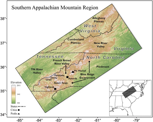
This research focuses on the SAM, a mid-latitude mountain region that exhibits much hydroclimatic variability, including the driest and wettest locations in the interior southeastern U.S. (SCO-NC 2015). Figure 1 shows the complex topographic distribution of ridges, valleys, and plateaus that stretch from northern Georgia to southern West Virginia in the SAM region. The general southwest to northeast orientation of ridges influences the distribution and intensity of precipitation across the region (Konrad 1996). Mean annual precipitation ranges from roughly 900 mm in various rain-shadowed valleys to nearly 2500 mm (Kelly et al. 2012) on prominent ridgelines, which are directly exposed to moisture advection from the Atlantic Ocean and Gulf of Mexico. Although the SAM is generally considered a water-rich environment due to its location in a humid subtropical climate, the occurrence of drought over the last several decades in addition to the unprecedented population growth across the southeastern U.S. has increased the demand for water resources across many sectors (Sun et al. 2013). When coupled with the occurrence of inter-basin hydroclimatic variability in the different topographic regions shown in Figure 1 and the concern for future stress on the water supply, the SAM is an ideal location for conducting a detailed spatial analysis of daily precipitation patterns.

Figure 1. Elevation and distribution of topographic regions across the southern Appalachian Mountains.

2.2. Precipitation data

Many studies have used regression-based analysis to examine the spatial pattern of precipitation with various topographic attributes as a predictor (Hevesi, Istok, and Flint 1992; Basist, Bell, and Meentemeyer 1994; Konrad 1996; Perry and Konrad 2006). However, they are subject to the limitation of station locations. Modeling approaches have improved in recent decades, such that spatially gridded and continuous precipitation estimates with improved accuracies are readily available. Specifically, multi-sensor precipitation estimation and the parameter-elevation relationships on independent slopes model (PRISM) estimates capture the current state of spatial climate patterns in the United States and offer physiographically sensitive estimates of precipitation (Daly et al. 2008; Zhang et al. 2011).

This study utilizes gridded daily precipitation estimates from PRISM (Prism Climate Group 2015). They are provided at a 4 × 4 km resolution over the U.S. PRISM estimates are particularly suited to studies in mountainous terrain because a climatically aided interpolation is used to generate them. Observations from 13,000 surface stations are incorporated into a regression model and then weighted according to physiographic characteristics that influence precipitation development. Multi-sensor precipitation estimates (MPE) are also utilized since 2002 in order to refine the precipitation estimates according to gauge-corrected radar observations. Daly et al. (2008) provide more details on the PRISM model and others have independently evaluated its performance in estimating precipitation (Currier, Thorson, and Lundquist 2017).

While the PRISM estimates have many advantages for modeling precipitation in mountainous terrain, there are several limitations and uncertainties that should be acknowledged when using any gridded precipitation product. Gridded rainfall products frequently underestimate heavy precipitation events and overestimate light precipitation (Chen and Knutson 2008; King, Alexander, and Donat 2013). Consequently, rainfall extremes in the gridded product tend to provide a smoothed characterization of the magnitude of the actual event (Tozer, Kiem, and Verdon-Kidd 2012). This effect can be amplified in areas of mountainous terrain (Chubb et al. 2016). Grid cell values represent an average aerial estimate of the raw values at a given scale and do not adequately reflect the sub-grid scale rainfall response to topographic complexity (Wootten and Boyles 2014). Some caution is therefore warranted in the interpretation of research results that are derived from gridded precipitation estimates.

Daily PRISM estimates were collected for this study from 2002 to 2014 for the months of June, July, and August. This daily time series identifies spatial patterns of precipitation that characterize the recent warm season hydroclimatology of the region. There is considerable seasonal variability in precipitation totals, so it provides a short term, 12-year climatology. The insight gained from this study characterizes the most recent period of hydroclimate extremes and does not reflect multidecadal variability.

2.3. Precipitation classification and visualization

Hydroclimate patterns are commonly conveyed in the form of means and ranges over a time period. However, the impacts of hydroclimate variability are tied to the nature of precipitation events on a daily scale, and how frequently different types of events are observed. One task that may help to unravel the complexity of the hydroclimate is to disaggregate the average precipitation over a given period (e.g. season) into the frequencies of different types or classes of daily precipitation events, from days with no precipitation to days with heavy precipitation. It is the occurrence or frequency of these events on a daily basis that will aid the identification of areas across mountain catchments where hydroclimatic extremes such as drought or heavy rainfall are likely to develop.

In order to show these precipitation metrics visually across the landscape, two attributes of the precipitation regime are calculated using a local operation over each grid cell in the SAM. First, the average summer season precipitation is determined through a summation of the daily precipitation totals across a season. Second, frequencies in the occurrence of different intensities of precipitation events are calculated for each grid cell and then divided by the number of seasons to estimate the seasonal return period (i.e. how frequently each precipitation type typically occurs during the summer).

Precipitation events are separated into four different event types: very light (0.25–2.54 mm), light (2.55–12.7 mm), moderate (12.8–38.1 mm), and heavy (≥38.1 mm). We used a series of sensitivity tests in combination with the suggested intensity thresholds from other hydroclimate research (Wootten and Boyles 2014) in the southeastern U.S. to derive these classes. The event type thresholds provide a specific focus on the light precipitation regime, which plays an important role in freshwater supply across many mountain regions. The thresholds were also chosen in order to isolate the most extreme precipitation events in the heaviest category.

A visualization is used to explore and interpret the spatial patterns for each precipitation event type. First, each raster surface of the return period for the precipitation event types is overlain on the 3D terrain model in Google Earth (Google Inc. 2016). Google Earth provides a web-based virtual globe for simple visualizations of raster data, and scientists have increasingly used its capability to communicate research findings (Goodchild 2008; Yu and Gong 2012). Its interface offers the user an opportunity to engage and interact with the precipitation surface by manually panning and zooming over the virtual globe at a fine spatial resolution. The user can explore precipitation patterns across different topographic settings from any height or perspective, and can utilize this capability as a mechanism for hypothesis generation (Butler 2006). For example, users can hypothesize how the distribution of precipitation events over different topographic regions is likely to influence the spatial pattern and composition of the resulting hydroclimatic regions in a statistical cluster analysis.

There are cognitive limitations to the visualization of geospatial data in a 3D environment (Slocum et al. 2001). For example, much research has identified the use of oblique 3D views with overlaid raster data as problematic for map interpretation and reading (Elmqvist and Tsigas 2008). Occlusion limits the perspective of the user and is particularly challenging when the objective is to discern regional scale patterns. However, this application is interactive, and it is used for exploratory visualization of precipitation patterns at local scales.

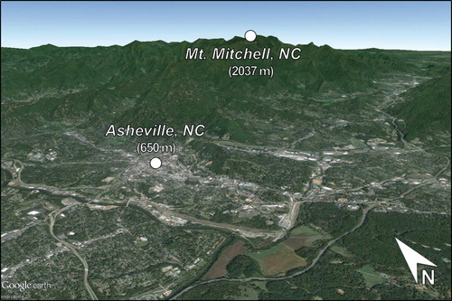
In this study, we present multiple visualizations of the precipitation pattern across the region using the 3D perspective in Figure 2. The perspective is an example of an east facing topographic transect from Asheville to Mt. Mitchell in western NC. This transect is marked by much topographic and climatic variability. Elevation increases more than 1300 m in the 38 km straight-line distance from the French Broad Valley in the foreground to the summits of the Black Mountain range in the background. Much of the ridgeline along the Black Mountain range is also exposed to moisture advection from the southeast. As a result of this exposure, average summer precipitation at Mt. Mitchell is greater than 450 mm. Asheville is situated in the rain-shadowed French Broad River valley located further west and has an average summer precipitation of 254 mm (Arguez et al. 2010).

Figure 2. Google Earth scene across a topographic transect from Asheville, NC, in the valley bottom, to Mt. Mitchell, across the ridgeline in the background. Photographic imagery Copyright 2016. Image: Landsat. Data: SIO, NOAA, U.S. Navy, NGA, GEBCO.

2.4. Cluster analysis and validation

In this study, cluster analysis is used to recast the complex spatial structure of hydroclimatic patterns into readily identifiable and interpretable regions that exhibit similarities in precipitation. Although there are other examples of similar grouping applications to identify hydroclimate subregions (Zambreski et al. 2018), cluster analysis is a very common technique in climate research to arrange data into homogenous groups around a centroid or spatial measure of central tendency (Fovell 1997; Carvalho et al. 2016). It maximizes the difference between clusters and minimizes the difference within clusters by calculating a minimum distance measurement between the centroid and each observation in the data space (Kalkstein, Tan, and Skindlov 1987; Konrad 1997). Depending on the type of algorithm that is chosen, each grid cell is examined to determine its Euclidean distance from other cells. As grid cells are continually assigned to centroids that share the most similar characteristics, this process is repeated until the finalized clusters are achieved (Wilks 2011). At this stage, its output is rendered as a static plot in two dimensions and traditionally serves as a useful tool for both exploration and interpretation of the resulting regions (Stooksbury and Michaels 1991).

There are several clustering algorithms suitable for determining groups in climate data. We compare three standard partitioning algorithms using programs for K-means, K-medoids (PAM), and clustering large applications (CLARA). The specific parameters of each algorithm are discussed in detail in Maechler et al. (2013) and based on the work of Kaufman and Rousseeuw (1990). We chose these algorithms due to their simplicity; they require that each precipitation variable is examined over each grid cell and compared with the centroid of a predetermined number of clusters (Hartigan and Wong 1979).

Partitioning approaches, like k-means or k-medoids, are computationally efficient (Wilks 2011). The grid cells are iteratively relocated to different clusters, so they provide a flexible way to show the most similar groupings as the algorithm compares each observation’s similarity in the data space. As opposed to hierarchical clustering algorithms, partitioning methods produce hard cluster boundaries that are easier to interpret. They are not nested within larger hierarchical structures of the data space and thus avoid some of the interpretation problems associated with fuzzy cluster boundaries (Fovell and Fovell 1993). Since the algorithm for k-means uses the mean value to determine the centroid locations for each cluster, it is sensitive to outliers within the data space. We also compare the performance of a k-medoids (e.g. PAM, CLARA) approach, which uses the median value to determine the centroid locations, and is thus not sensitive to the outliers.

There are several limitations to the clustering techniques that are described above. First, the requirement to choose the k amount of clusters is a challenging part in the initialization of these algorithms. Although hierarchical algorithms will automatically converge on the best number of clusters (Kalkstein, Tan, and Skindlov 1987; Shinker 2010), interpretation can be difficult due to the complexity and number of geographic regions that are identified (Fovell and Fovell 1993). In this study, sample routines for each application are implemented with k = 5, 6, and 7 clusters to assess the sensitivity of the resulting hydroclimatic regions to variations in each algorithm. We also examined the performance of k = 3 and 4 cluster groupings, though the results are omitted from the discussion because the generality of the regions did not reflect the hydroclimatic and topographic complexity of the study area. Second, the resulting regions, or cluster boundaries, are sensitive to the spatial domain that is used to derive them and may deviate a bit from the patterns that are exhibited in the broad-scale regional hydroclimate of the southeast. The spatial patterns should be interpreted with caution.

In order to carry out the analysis, the frequency of precipitation event types is standardized so that each exhibits an equal weighting as input variables in the cluster analysis (Wilks 2011). Standardized frequencies are calculated based on the daily occurrence of each precipitation event type observed over all grid cells. For each grid cell, the mean frequency of the precipitation event types is subtracted from the observed frequency and then divided by the standard deviation. The standardized frequency of different precipitation events thus provides a dimensionless measure of their occurrence across the region relative to the mean.

3. Results

3.1. Precipitation climatology

A comparison of summer season precipitation variables is presented in Figure 3. There is much variability in the spatial pattern of average summer precipitation. On a local scale, rain-shadowed valleys receive less precipitation than the adjacent ridges. Figure 1 provides the associated topographic references. The larger valleys (e.g. the French Broad, New, and TN river valleys) are the driest, receiving less than 254 mm of precipitation in places. These valleys are shielded from moisture advection in nearly every direction, making them the driest locations in the interior southeastern US. Higher precipitation amounts (>381 mm (15 in)) are found along the western slopes of the Allegheny Plateau, Cumberland Plateau, and Great Smoky Mountains, as these areas are exposed to moisture advection from the west and northwest. However, the most precipitation (>508 mm (20 in)) occurs in the Blue Ridge region, which is directly exposed to moisture advection from the south and southeast. This is especially the case along the southern Blue Ridge Escarpment in western NC, which is the wettest region in the interior southeastern US. The town of Highlands, located at the top of the escarpment, in fact, holds a record for the greatest one-day precipitation event (537.21 mm (21.15 in)) in NC (SCO-NC 2015). These patterns line up well with previously documented orographic precipitation patterns (Konrad 1996; Kelly et al. 2012; Papalexiou, AghaKouchak, and Foufoula-Georgiou 2018).

Figure 3. (a) Average summer precipitation derived from daily, gridded PRISM precipitation estimates. (b) Average daily intensity of precipitation is calculated using all non-zero precipitation days. (c) Average summer maximum precipitation. (d) Frequency of days per season with precipitation in each grid cell.

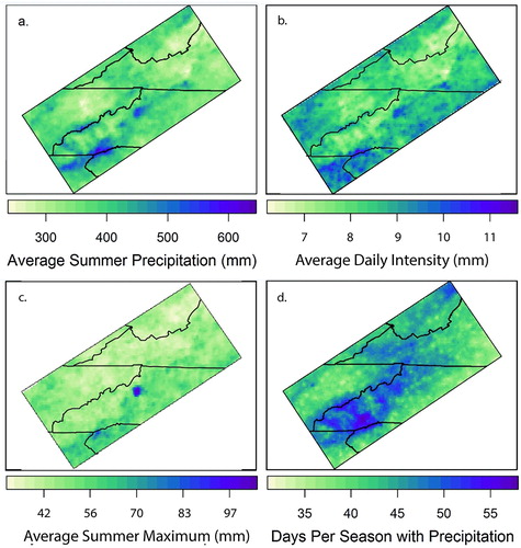
The frequencies of seasonal precipitation also exhibit much spatial variability, yet the spatial pattern is a bit different from the seasonal averages. Precipitation is least frequent in the TN Valley and the NC-VA Piedmont, occurring less than 35 days per season. Increased frequencies of precipitation (40 days per season) are found in the French Broad and New River valleys. Both of these valleys are situated in the interior of the SAM and display a higher elevation. Precipitation occurs frequently at 45–50 days per season across areas of higher elevation (>1000 m) in southwestern NC, northwestern NC, the Cumberland Plateau in far southwestern VA, and the Allegheny Plateau in WV. Precipitation is most frequent across the exposed ridgelines in western NC, which includes the Great Smoky Mountains, Balsam and Black Mountain ranges, and the southern Blue Ridge Escarpment. There are more than 55 days with precipitation in these areas, which is more than half of the days during the summer season. This pattern also includes several of the narrow interior river valleys in southwestern NC and indicates that portions of the SAM, including some areas with lower average summer precipitation, are frequently wetted over the course of the summer.

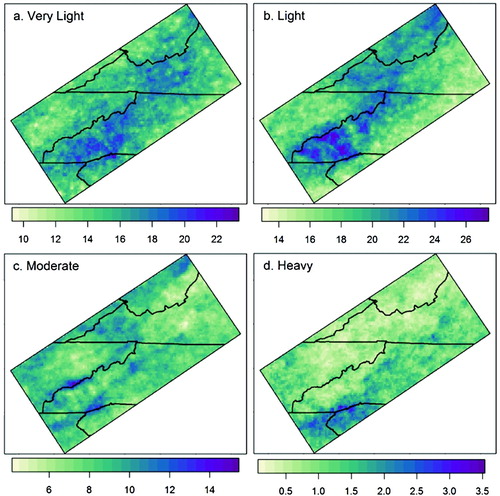
The spatial patterns of the return period for each precipitation event type are presented in Figure 4. Many of these patterns have a connection with the terrain in Figure 1. They also exhibit the expected j-shaped or bell shaped characteristics of the distribution of daily precipitation occurrence (Papalexiou and Koutsoyiannis 2016). For example, very light and light precipitation events occur most frequently, and they are widespread among many of the topographic regions. Days with very light precipitation (18–20 days per season) are most frequent in high elevation regions, which includes the Blue Ridge Escarpment and the Balsam and Black Mountain ranges. However, they are also frequent in various valleys, including the New River and French Broad valleys. This pattern shares much in common to the days with light precipitation, which occurs even more frequently across these regions. Combined, very light and light precipitation characterize nearly 50% of the total precipitation events across the high elevations in the SAM during the summer season. Days with very light and light precipitation events are least frequent in the Piedmont and TN river valley (<15 days per season). We expect that a cluster analysis will identify ridgelines and higher elevation valleys within the interior of the SAM as a distinct hydroclimatic zone, which features higher frequencies of the lighter events.

Figure 4. Comparison of the average number of days per season with (a) very light, (b) light, (c) moderate, and (d) heavy precipitation events.

Moderate and heavy precipitation events occur least frequently across the SAM. Moderate events are most common (12–14 days per season) along the northwestern boundary of the SAM and the southeastern slopes of the Blue Ridge Escarpment. Exposed ridgelines along interior portions of the SAM, including the Great Smoky Mountains, also exhibit relatively high occurrences of moderate precipitation. They are the least likely to occur throughout the intervening valleys and the adjacent Piedmont. Heavy precipitation events are the least commonly occurring across the SAM. The highest frequencies (2–4 days per season) are located along the Blue Ridge Escarpment and the adjacent Piedmont. A cluster analysis will therefore likely identify the Blue Ridge Escarpment and sections of the Piedmont as a distinct hydroclimatic zone, which features higher frequencies of both moderate and heavy precipitation events. It will also likely identify northwestern areas as a distinct hydroclimatic zone that features high frequencies of light and moderate precipitation and low frequencies of heavy events.

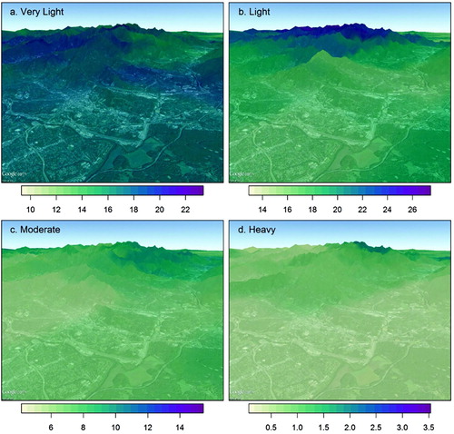
A visualization of the spatial pattern of the return period for each precipitation event type is presented in Figure 5 in order to further hypothesize which topographic regions will share similar precipitation characteristics. Precipitation events occur most frequently for all event types along the exposed ridgeline and higher elevations in the background. There are, however, some variations in the altitudinal changes across each type. There is only a slight decrease in the frequencies of very light precipitation from the ridge top (18 events per season) down to the valley bottom (16 events per season). Light, moderate, and heavy precipitation events show much greater changes in frequency across the altitudinal gradient. Light precipitation events are most frequent across the ridge tops (>26 days per season) and decrease to 15 days per season in the valley bottom. Moderate precipitation events occur 10 days per season across the exposed southeastern ridge tops and less than 6 days per season in the river valley. Heavy precipitation events occur 2 days per season across the highest ridge tops and occur less than 1 day per season in the valley bottom. The visualization emphasizes the dry summer season conditions that are typically found in the valley and the relative high frequency of precipitation events along the ridgelines. Panning and zooming across the terrain of the entire study area confirmed a similar pattern, to varying degrees. A cluster analysis of precipitation event types should therefore delineate hydroclimatic regions that highlight the separate precipitation regimes between the valleys and ridge tops in the SAM.

Figure 5. Visualization depicting the average number of days per season with (a) very light, (b) light, (c) moderate, and (d) heavy precipitation events across the topographic transect. Photographic imagery Copyright 2016. Image: Landsat. Data: SIO, NOAA, U.S. Navy, NGA, GEBCO.

3.2. Cluster results and performance

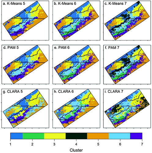
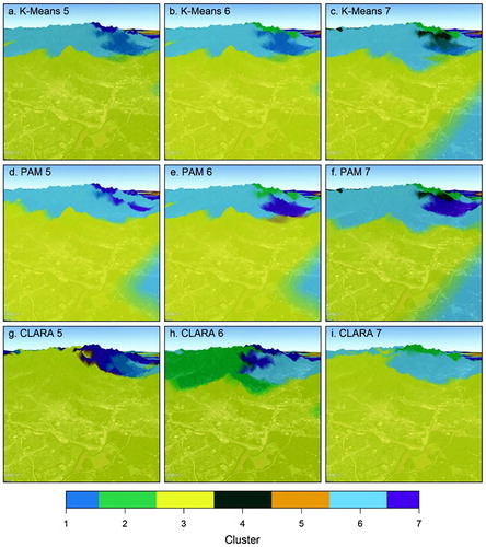
The results from K-Means, PAM, and CLARA clustering algorithms are presented in Figure 6. Increasing the amount of clusters in each type adds spatial complexity to the resulting regions. Each of the clustering procedures with seven regions introduces unnecessary interdigitation between grid cells with opposing cluster membership, increases noise or patchiness, and simultaneously reduces the overall interpretability of the hydroclimatic regions. For example, cluster four in CLARA 7 is not a contiguous geographic region with uniform topography, although its precipitation characteristics are similar. It instead interrupts the contiguity of cluster two which would otherwise span the entirety of the Piedmont. The interdigitation between the two clusters is unnecessary because the hydroclimatic regimes between the two clusters are likely similar in such close geographic proximity. Interdigitation and cluster noise are also noticeable across the SAM in K-means 6, PAM 6, and CLARA 6. In our visual assessment, cluster results with five regions are more cohesive and the regional patterns are easier to interpret geographically. For example, cluster five generally extends over the entire Piedmont, while cluster three is located across the French Broad, New, and TN River Valleys.

Figure 6. Performance comparison of clustering results with five (left column), six (center column), and seven (right column) clusters. Clustering results from K-means (upper row), PAM (center row), and CLARA (lower row) clustering algorithms are compared. A single legend is used for all combinations; however, certain cluster numbers (e.g. 3, 5) will not be used in each column.

Interior cluster validation statistics are used in order to determine which algorithms perform the best (Brock et al. 2008). Three statistical indices are used to examine spatial characteristics of the clusters (Table 1). First, a connectivity index, ranging from zero to ∞, is used to measure the extent to which the grid cells are placed in the same cluster as the nearest neighbor grid cells. Connectivity is a characteristic that can improve the interpretability of the resulting regions as long as the intra-cluster precipitation characteristics remain homogenous as the regions are delineated (Arguez et al. 2016). Lower values indicate a higher degree of connectivity for large groups of grid cells that are located in similar topographic environments. Clustering algorithms for K-Means 5 and PAM 5 exhibit the highest regional connectivity, while PAM 7 and CLARA 7 exhibit the least connectivity.

Table 1. Internal validation statistics comparing five, six, and seven clusters for K-Means, PAM, and CLARA clustering algorithms.

No. of clusters	5	6	7
K-Means
Connectivity	1410	1729	1863
Dunn	0 . 0121	0.0092	0.0103
Silhouette	0 . 2507	0.2358	0.2249
PAM
Connectivity	1598	1838	2054
Dunn	0.0065	0.0103	0.0048
Silhouette	0 . 2406	0.2280	0.2078
CLARA
Connectivity	1804	1896	2249
Dunn	0 . 0122	0.0066	0.0092
Silhouette	0.2012	0.2008	0.1693

Notes: Validation statistics include the connectivity index, Dunn index, and silhouette width of each cluster. The highest ranking statistics are bolded to show the best clustering performance.

Second, the Dunn index, described in detail in Dunn (1974), and the silhouette width (Rousseeuw 1987) are used to combine statistical measures of cluster compactness and separation into a single index. Compactness is a characteristic of cluster homogeneity and it is calculated based on the intra-cluster variance of grid cell values. Separation is determined by measuring the distance between cluster centroids. Compactness increases along with the amount of clusters while separation decreases as the regions become interdigitated (Brock et al. 2008). The Dunn index measures this relationship as a ratio between zero and ∞, with maximum values indicating good cluster performance.

In Table 1, PAM 5 and PAM 7 exhibit the lowest Dunn index value, indicating an uneven relationship between the degree of regional compactness and separation. Both clustering algorithms result in hydroclimatic regions with elongated and sinuous spatial patterns, which are difficult to interpret in Figure 6. CLARA 5 and K-Means 5 exhibit the greatest Dunn index values, indicating that hydroclimatic regions have compact cluster shapes and relatively even distances between cluster members and cluster centroids.

Silhouette widths range from −1, which are poorly clustered, to 1, which indicates good clustering performance. In Table 1, all clustering algorithms have positive silhouette widths. K-Means 5 and PAM 5, however, exhibit the greatest silhouette widths, indicating a higher degree of confidence in the cluster assignment for each grid cell (Brock et al. 2008). Results from the interior cluster validation demonstrate that K-Means 5 and PAM 5 provide the most ideal representation of hydroclimatic regions across the SAM.

3.3. Identification of hydroclimatic regions

A visualization is used to subjectively assess and inform the choice of the best cluster analysis from the internal cluster validation (Figure 7). This is a common technique to determine the appropriate amount of clusters and confirm whether they align with the validation statistics described above (Zhang, Moges, and Block 2016). 3D perspectives were examined along several topographic transects in the region where there is much change in precipitation, including the transect in Figure 2. The K-Means 7, PAM 7, and CLARA 7 patterns are difficult to interpret because of the unrealistic amount of clusters. It is unlikely that three or more hydroclimatic regions are present over the short transect distance from the valley bottom up to the ridge tops. The clusters are also highly interdigitated and patchy across the steeper slopes in the background, insinuating that multiple hydroclimatic regimes are present in similar topographic environments. K-Means 6, PAM 6, and CLARA 6 present a similar pattern. Therefore, a reduced amount of clusters is desired to simplify the spatial complexity of the hydroclimatic regions. Patterns in K-Means 5 and PAM 5 are more readily perceived due to their higher connectivity. Although K-Means is ranked the best according to its validation statistics, panning and zooming across the region reveals that PAM 5 exhibits the most coherency and organization across the landscape.

Figure 7. Visualizations of the nine clustering results are subjectively compared across the transect. The visualization allows the user to pan, zoom, and tilt across different topographic regions of the SAM. Photographic imagery Copyright 2016. Image: Landsat. Data: SIO, NOAA, U.S. Navy, NGA, GEBCO.

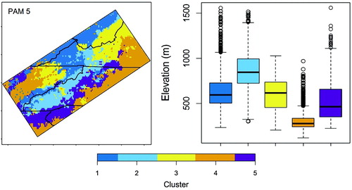
The regions (i.e. clusters) in PAM 5 align well with the topographic environments across the SAM (Figure 8). First, zone one spans across the Allegheny Plateau, Cumberland Plateau, and portions of the Great Smoky Mountains (compare with Figure 1). Region two contains much of the interior high elevations, including the Great Smoky Mountains, Balsam and Black Mountain ranges. Region three is located across portions of the low-lying French Broad, TN, and New River valleys. Further southeast, region four contains the Blue Ridge Escarpment and extends a short distance into the NC-VA Piedmont. The Piedmont is denoted as region five because it spans across portions of central NC, VA, and TN. Region five also contains a disjoined area, which is separately located in the TN valley, and shares similar precipitation characteristics to the Piedmont. Given its superior performance in our visual assessment and alignment of regions with topographic features, PAM 5 best characterizes the regional patterns of precipitation.

Figure 8. PAM 5 clustering results with 5 clusters or hydroclimatic regions and their elevation descriptive statistics.

4. Discussion

Figure 9 summarizes the differences in the hydroclimatic regimes across the SAM using the clusters in PAM 5. The average occurrence of the precipitation events is computed as a standardized frequency for each zone to reveal its hydroclimatic character. Each zone is also given a descriptive regional name that characterizes the underlying topographic environment. They are described in order of their geographic location from northwest to southeast. First, the NW Slopes and Plateau region is located along the northwestern boundary of the SAM and encompasses the Allegheny Plateau, Cumberland Plateau, and the Great Smoky Mountains. It exhibits relatively high standardized frequencies of light and moderate precipitation and low standardized frequencies of very light and heavy precipitation. It is also the second wettest region of the study area, with 386 mm average rainfall during the warm season.

Figure 9. Composite bar plots are used to determine the precipitation characteristics for each hydroclimatic region. Average standardized frequencies for very light (VL), light (L), moderate (M), and heavy (H) precipitation are computed to reveal cross-regional differences in hydroclimatic character.

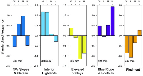
The adjacent Interior Highlands region displays the highest elevations and includes portions of the Balsam and Black Mountain ranges and the Great Smoky Mountains. Relative to the other regions, very light and light precipitation occur more frequently there compared to the moderate or heavy events. This finding is supported by Konrad (1996), who found a strong correlation between elevation and light precipitation, and weaker relationships between elevation and moderate or heavy precipitation. In a more recent study, however, Papalexiou, AghaKouchak, and Foufoula-Georgiou (2018) identified a clear relationship between elevation and heavy precipitation. The Interior Highlands is the third wettest region overall (378 mm). Evidence suggests that the persistent light rainfall regime that occurs on a near-daily basis serves as a hydroclimatic lifeline during the warm season (Wilson and Barros 2014), buffering the highest elevations from the threat of meteorological drought during periods when the lower regions suffer from extended dry spells (Sugg and Konrad 2017).

The Elevated Valleys region identifies three broad valleys in the interior of the SAM: the French Broad, New, and TN River valleys. Precipitation is less frequent in the Elevated Valleys compared to the adjacent surrounding regions. However, it is more frequent than in the Piedmont. Days with moderate or heavy precipitation are the least frequent overall. The Elevated Valleys are nested within surrounding regions and are thereby sheltered in many directions by mountain slopes, making this the driest region (305 mm).

The remaining two hydroclimatic regions are situated along the southeastern side of the SAM. The Blue Ridge and Foothills is the wettest region overall (424 mm). It is marked by contiguous and steep, southeastern facing slopes of the Blue Ridge Escarpment, which extend into the adjacent Piedmont region. With the exception of light rainfall, all precipitation event types are frequent in the Blue Ridge and Foothills region. Heavy precipitation occurs most frequently in this region compared to the others. In the Piedmont region, very light and light precipitation events are the least frequent compared to the other hydroclimatic regions. Moderate precipitation is more frequent than in the Elevated Valleys. The Piedmont region has the second highest occurrence of heavy precipitation events. It is the second driest region overall (347 mm).

5. Conclusion

Descriptive models that reduce the complexity of mountain hydroclimate are easily visualized over a 3D virtual globe. This analysis of hydroclimatic patterns provided new information about the frequency and location of daily precipitation during the warm season in the SAM region. Unique hydroclimatic regions that exhibit commonalities in the precipitation regime were identified by using gridded climate data as an input to a K-medoids cluster analysis.

Although the average seasonal rainfall was similar (305–424 mm) between the hydroclimatic regions, the delivery of rainfall varied according to the frequency of different daily precipitation events. This finding explains the difference in hydroclimatic character between geographic regions of the SAM, and can be used to understand where extremes are likely to occur across the landscape. As the climate continues to warm, the Elevated Valleys and Piedmont regions are likely to be the most vulnerable to drought when compared with other regions due to the low frequencies of all precipitation types there. On the other hand, some high elevation regions may exhibit resilience to drought due to the higher frequencies of precipitation. Research is needed to compare the observed occurrence of precipitation-related hazards, such as drought and flash flooding, in context with the precipitation frequencies identified in this study and to reduce the uncertainties that are tied to spatial modeling of precipitation in mountainous terrain.

There are several practical applications of this research for different user groups, like water resource planners, forecasters, and researchers. First, the southeastern U.S. is generally a water-rich environment. Yet the occurrence of drought (Maxwell and Soulé 2009; Ortegren et al. 2011) in addition to the unprecedented population growth across the region has increased the demand for water resources across many sectors (Manuel 2008; Sun et al. 2013). This creates a need for stakeholders to better understand how the existing spatial footprint of precipitation might lead to future hazards. Second, atmospheric circulation patterns and teleconnections are tied to the development of wet and dry regimes (Sugg and Konrad 2017; Engström and Waylen 2018), yet there are many uncertainties in the future predictions that are derived from downscaled climate models (Wootten et al. 2014). Specifically, there is a need to better understand circulation-precipitation relationships at the daily scale in global mountain regions in order to better inform the predictions. Finally, the SAM region is part of the warming hole, a broader region across the U.S. that has not followed global or national level climate predictions (Pan et al. 2004; Meehl, Arblaster, and Branstator 2012; Ellenburg et al. 2016). This research provides a useful example of examining wide-ranging regional hydroclimatic variability in the context of global climate trends. The new map of hydroclimatic regions that was developed in this study provides a descriptive model of recent hydroclimatic variability in the SAM and provides a baseline for understanding how precipitation-related hazards may be changing in this mid-latitude mountain region.

Acknowledgements

The data that support the findings of this study are openly available from the PRISM Climate Group at Oregon State University at [http://www.prism.oregonstate.edu/], AN81d.

Disclosure statement

No potential conflict of interest was reported by the authors.

References

- Arguez, Anthony, Imke Durre, Scott Applequist, Mike Squires, Russell Vose, Xungang Yin, and Rocky Bilotta. 2010. “NOAA’s U.S. Climate Normals (1981-2010).” NOAA National Centers for Environmental Information. doi:10.7289/V5PN93JP.
- Barros, Ana P., and Dennis P. Lettenmaier. 1993. “Dynamic Modeling of the Spatial Distribution of Precipitation in Remote Mountainous Areas.” Monthly Weather Review. doi:10.1175/1520-0493(1993)121<1195:DMOTSD>2.0.CO;2.
- Barry, Roger G. 2008. Mountain Weather and Climate. 3rd ed. Cambridge: Cambridge University Press.
- Basist, Alan, Gerald D. Bell, and Vernon Meentemeyer. 1994. “Statistical Relationships Between Topography and Precipitation Patterns.” Journal of Climate 7: 1305–1315. doi:10.1175/1520-0442(1994)007<1305:SRBTAP>2.0.CO;2.
- Brock, Guy, Vasyl Pihur, Susmita Datta, and Somnath Datta. 2008. “ClValid, an R Package for Cluster Validation.” Journal of Statistical Software 25 (4). http://cran.us.r-project.org/web/packages/clValid/vignettes/clValid.pdf VN-readcube.com. doi: 10.18637/jss.v025.i04
- Butler, Declan. 2006. “The Web-wide World.” Nature 439 (16): 776–778. doi: 10.1038/439776a
- Carvalho, M. J., P. Melo-Gonçalves, J. C. Teixeira, and A. Rocha. 2016. “Regionalization of Europe Based on a K-Means Cluster Analysis of the Climate Change of Temperatures and Precipitation.” Physics and Chemistry of the Earth 94: 22–28. doi:10.1016/j.pce.2016.05.001.
- Chen, Cheng T., and Thomas Knutson. 2008. “On the Verification and Comparison of Extreme Rainfall Indices from Climate Models.” Journal of Climate 21 (7): 1605–1621. doi:10.1175/2007JCLI1494.1.
- Christensen, J. H., K. Krishna Kumar, E. Aldrian, S.-I. An, I. F. A. Cavalcanti, M. de Castro, W. Dong, et al. 2013. “Climate Phenomena and Their Relevance for Future Regional Climate Change.” Climate Change 2013: The Physical Science Basis. Contribution of Working Group I to the Fifth Assessment Report of the Intergovernmental Panel on Climate Change. doi:10.1017/CBO9781107415324.028.
- Chubb, Thomas H., Michael J. Manton, Steven T. Siems, and Andrew D. Peace. 2016. “Evaluation of the AWAP Daily Precipitation Spatial Analysis with an Independent Gauge Network in the Snowy Mountains.” Journal of Southern Hemisphere Earth Systems Science 66: 55–67. doi: 10.22499/3.6601.006
- Currier, William Ryan, Theodore Thorson, and Jessica D. Lundquist. 2017. “Independent Evaluation of Frozen Precipitation from WRF and PRISM in the Olympic Mountains.” Journal of Hydrometeorology 18 (10): 2681–2703. doi:10.1175/JHM-D-17-0026.1.
- Daly, Christopher, Michael Halbleib, Joseph I. Smith, Wayne P. Gibson, Matthew K. Doggett, George H. Taylor, and Phillip P. Pasteris. 2008. “Physiographically Sensitive Mapping of Climatological Temperature and Precipitation Across the Conterminous United States.” International Journal of Climatology 28 (15): 2031–2064. doi:10.1002/joc.1688.
- Dunn, J. C. 1974. “Well-separated Clusters and Optimal Fuzzy Partitions.” Journal of Cybernetics 4 (1): 95–104. doi: 10.1080/01969727408546059
- Ellenburg, W. L., R. T. McNider, J. F. Cruise, and John R. Christy. 2016. “Towards an Understanding of the Twentieth-century Cooling Trend in the Southeastern United States: Biogeophysical Impacts of Land-use Change.” Earth Interactions 20 (18). doi:10.1175/EI-D-15-0038.1.
- Elmqvist, Niklas, and Philippas Tsigas. 2008. “A Taxonomy of 3D Occlusion Management for Visualization.” IEEE Transactions on Visualization and Computer Graphics 14 (5): 1095–1109. doi: 10.1109/TVCG.2008.59
- Engström, Johanna, and Peter Waylen. 2017. “The Changing Hydroclimatology of Southeastern U.S.” Journal of Hydrology 548: 16–23. doi:10.1016/j.jhydrol.2017.02.039.
- Engström, Johanna, and Peter Waylen. 2018. “Drivers of Long-Term Precipitation and Runoff Variability in the Southeastern USA.” Theoretical and Applied Climatology, 1133–1146. doi:10.1007/s00704-016-2030-4.
- Fovell, Robert G. 1997. “Consensus Clustering of U.S. Temperature and Precipitation Data.” Journal of Climate 10 (6): 1405–1427. doi: 10.1175/1520-0442(1997)010<1405:CCOUST>2.0.CO;2
- Fovell, Robert G., and Mei-Ying C. Fovell. 1993. “Climate Zones of the Coterminous United States Defined Using Clutser Analysis.” Journal of Climate 6: 2103–2135. doi: 10.1175/1520-0442(1993)006<2103:CZOTCU>2.0.CO;2
- Frame, Jeffrey, and Paul Markowski. 2006. “The Interaction of Simulated Squall Lines with Idealized Mountain Ridges.” Monthly Weather Review 134 (7): 1919–1941. doi:10.1175/MWR3157.1.
- Goodchild, M. F. 2008. “The Use Cases of Digital Earth.” International Journal of Digital Earth 1 (1): 31–42. doi:10.1080/17538940701782528.
- Hartigan, J. A., and M. A. Wong. 1979. “Algorithm AS 136 : A K-Means Clustering Algorithm.” Journal of the Royal Statistical Society. Series C (Applied Statistics) 28 (1): 100–108.
- Hevesi, Joseph A., Jonathan D. Istok, and Alan L. Flint. 1992. “Precipitation Estimation in Mountainous Terrain Using Multivariate Geostatistics. Part I: Structural Analysis.” Journal of Applied Meteorology 31 (7): 661–676. doi: 10.1175/1520-0450(1992)031<0661:PEIMTU>2.0.CO;2
- Kahya, E., and J. Dracup. 1993. “US Streamflow Patterns in Relation to the El Nino/Southern Oscillation.” Water Resources Research. http://www.akademi.itu.edu.tr/kahyae/DosyaGetir/57273/WRR94.pdf%5Cnpapers2://publication/uuid/57F00DC9-AAB0-4EEB-B5CD-C768637D0755.
- Kalkstein, Laurence S., Guanri Tan, and Jon A. Skindlov. 1987. “An Evaluation of Three Clustering Procedures for Use in Synoptic Climatological Classification.” Journal of Climate and Applied Meteorology 26 (6): 717–730. doi: 10.1175/1520-0450(1987)026<0717:AEOTCP>2.0.CO;2
- Katz, Richard W., Marc B. Parlange, and Claudia Tebaldi. 2003. “Stochastic Modeling of the Effects of Large-scale Circulation on Daily Weather in the Southeastern U.S.” Climatic Change 60 (1–2): 189–216. doi:10.1023/A:1026054330406.
- Kaufman, L., and P. J. Rousseeuw. 1990. Finding Groups in Data: An Introduction to Cluster Analysis. New York: John Wiley & Sons, Inc.
- Kelly, Ginger M., L. Baker Perry, Brett F. Taubman, and Peter T. Soulé. 2012. “Synoptic Classification of 2009–2010 Precipitation Events in the Southern Appalachian Mountains, USA.” Climate Research 55 (1): 1–15. doi:10.3354/cr01116.
- King, Andrew D, Lisa V Alexander, and Markus G Donat. 2013. “The Efficacy of Using Gridded Data to Examine Extreme Rainfall Characteristics : A Case Study for Australia.” International Journal of Climatology 33: 2376–2387. doi:10.1002/joc.3588.
- Konrad, Charles E. 1996. “Relationships Between Precipitation Event Types and Topography in the Southern Blue Ridge Mountains of the Southeastern USA.” International Journal of Climatology 16 (January): 49–62. doi:10.1002/(SICI)1097-0088(199601)16:1<49::AID-JOC993>3.0.CO;2-D.
- Konrad, Charles E. 1997. “Synoptic-scale Features Associated with Warm Season Heavy Rainfall Over the Interior Southeastern United States.” Weather and Forecasting 12 (3): 557–571. doi: 10.1175/1520-0434(1997)012<0557:SSFAWW>2.0.CO;2
- Kramer, Randall A., and Jonathan I. Eisen-Hecht. 2002. “Estimating the Economic Value of Water Quality Protection in the Catawba River Basin.” Water Resources Research 38 (9): 21-1–21-10. doi:10.1029/2001WR000755.
- Lin, Yuh-Lang, Sen Chiao, Ting-An Wang, Michael L. Kaplan, and Ronald P. Weglarz. 2001. “Some Common Ingredients for Heavy Orographic Rainfall.” Weather and Forecasting 16 (6): 633–661. doi: 10.1175/1520-0434(2001)016<0633:SCIFHO>2.0.CO;2
- Maechler, M., P. Rousseeuw, A. Struyf, M. Hubert, and K. Hornik. 2013. “Package ‘Cluster’”.
- Manuel, John. 2008. “Drought in the Southeast: Lessons for Water Management.” Environmental Health Perspectives 116 (4): 168–171. doi: 10.1289/ehp.116-a168
- Maxwell, Justin T., and Peter T. Soulé. 2009. “United States Drought of 2007: Historical Perspectives.” Climate Research 38 (2): 95–104. doi:10.3354/cr00772.
- Meehl, Gerald A., Julie M. Arblaster, and Grant Branstator. 2012. “Mechanisms Contributing to the Warming Hole and the Consequent U.S. East-West Differential of Heat Extremes.” Journal of Climate 25 (18): 6394–6408. doi:10.1175/JCLI-D-11-00655.1.
- Nykanen, Deborah K., and Daniel Harris. 2003. “Orographic Influences on the Multiscale Statistical Properties of Precipitation.” Journal of Geophysical Research 108 (D8), doi:10.1029/2001JD001518.
- Ortegren, Jason T., Paul A. Knapp, Justin T. Maxwell, William P. Tyminski, and Peter T. Soulé. 2011. “Ocean–Atmosphere Influences on Low-frequency Warm-season Drought Variability in the Gulf Coast and Southeastern United States.” Journal of Applied Meteorology and Climatology 50 (6): 1177–1186. doi:10.1175/2010JAMC2566.1.
- Pan, Zaitao, Raymond W. Arritt, Eugene S. Takle, William J. Gutowski, Christopher J. Anderson, and Moti Segal. 2004. “Altered Hydrologic Feedback in a Warming Climate Introduces a ‘Warming Hole’.” Geophysical Research Letters 31 (17): 2–5. doi:10.1029/2004GL020528.
- Papalexiou, Simon Michael, Amir AghaKouchak, and Efi Foufoula-Georgiou. 2018. “A Diagnostic Framework for Understanding Climatology of Tails of Hourly Precipitation Extremes in the United States.” Water Resources Research, 6725–6738. doi:10.1029/2018WR022732.
- Papalexiou, Simon Michael, and Demetris Koutsoyiannis. 2016. “A Global Survey on the Seasonal Variation of the Marginal Distribution of Daily Precipitation.” Advances in Water Resources 94: 131–145. doi:10.1016/j.advwatres.2016.05.005.
- Perry, L. Baker, and Charles E. Konrad. 2006. “Relationships Between NW Flow Snowfall and Topography in the Southern Appalachians, USA.” Climate Research 32: 35–47. doi: 10.3354/cr032035
- Prism Climate Group. 2015. “Prism Gridded Climate Data.” Terms of Use. http://prism.oregonstate.edu.
- Rousseeuw, Peter J. 1987. “Silhouettes: A Graphical Aid to the Interpretation and Validation of Cluster Analysis.” Journal of Computational and Applied Mathematics 20: 53–65. doi:10.1016/0377-0427(87)90125-7.
- Ruhl, J. B. 2005. “Water Wars, Eastern Style: Divvying Up the Apalachicola-Chattahoochee-Flint River Basin.” Journal of Contemporary Water Research & Education 131 (May): 47–54. doi:10.1111/j.1936-704X.2005.mp131001008.x.
- SCO-NC. 2015. “Overview.” State Climate Office of North Carolina. http://www.nc-climate.ncsu.edu/climate/ncclimate.html.
- Shinker, Jacqueline J. 2010. “Visualizing Spatial Heterogeneity of Western U.S. Climate Variability.” Earth Interactions 14 (10): 1–15. doi:10.1175/2010EI323.1.
- Sinclair, Mark R., David S. Wratt, Roddy D. Henderson, and Warren R. Gray. 1997. “Factors Affecting the Distribution and Spillover of Precipitation in the Southern Alps of New Zealand – A Case Study.” Journal of Applied Meteorology 36 (5): 428–442. doi: 10.1175/1520-0450(1997)036<0428:FATDAS>2.0.CO;2
- Slocum, Terry A, Connie Blok, Bin Jiang, Alexandra Koussoulakou, Daniel R Montello, Sven Fuhrmann, and Nicholas R Hedley. 2001. “Cognitive and Usability Issues in Geovisualization.” Cartography and Geographic Information Science 28: 61–76. doi: 10.1559/152304001782173998
- Stooksbury, D. E., and P. J. Michaels. 1991. “Cluster Analysis of Southeastern U.S. Climate Stations.” Theoretical and Applied Climatology 44 (3–4): 143–150. doi: 10.1007/BF00868169
- Sugg, Johnathan W., and Charles E. Konrad. 2017. “Relating Warm Season Hydroclimatic Variability in the Southern Appalachians to Synoptic Weather Patterns Using Self-organizing Maps.” Climate Research 74: 145–160. doi: 10.3354/cr01493
- Sun, Ge, Peter V. Caldwell, Steven G. Mcnulty, Aris P. Georgakakos, Sankar Arumugam, James Cruise, Richard T. McNider, et al. 2013. Impacts of Climate Change and Variability on Water Resources in the Southeast USA.
- Tozer, C. R., A. S. Kiem, and D. C. Verdon-Kidd. 2012. “On the Uncertainties Associated with Using Gridded Rainfall Data as a Proxy for Observed.” Hydrology and Earth System Sciences 16: 1481–1499. doi:10.5194/hess-16-1481-2012.
- Wear, David, and John Greis. 2011. “The Southern Forest Resource Assessment: Summary Report. Gen. Tech. Rep. SRS-54.” 1–79.
- Wilks, Daniel S. 2011. Statistical Methods in the Atmospheric Sciences. 3rd ed. Academic Press. https://books.google.com/books?id=IJuCVtQ0ySIC&lr=&source=gbs_navlinks_s.
- Williams, Park, Benjamin Cook, Jason E. Smerdon, Daniel A. Bishop, Richard Seager, and Justin S. Mankin. 2017. “The 2016 Southeastern U.S. Drought: An Extreme Departure From Centennial Wetting and Cooling.” Journal of Geophysical Research: Atmospheres 122 (20): 10888–10905. doi:10.1002/2017JD027523.
- Wilson, Anna M., and Ana P. Barros. 2014. “An Investigation of Warm Rainfall Microphysics in the Southern Appalachians: Orographic Enhancement via Low-level Seeder–Feeder Interactions.” Journal of the Atmospheric Sciences, 1783–1805. doi:10.1175/JAS-D-13-0228.1.
- Wootten, Adrienne, and Ryan P. Boyles. 2014. “Comparison of NCEP Multisensor Precipitation Estimates with Independent Gauge Data Over the Eastern United States.” Journal of Applied Meteorology and Climatology 53: 2848–2862. doi:10.1175/JAMC-D-14-0034.1.
- Wootten, Adrienne, Kara Smith, Ryan Boyles, Adam Terando, Lydia Stefanova, Vasu Misra, Tom Smith, David Blodgett, and Fredrick Semazzi. 2014. Downscaled Climate Projections for the Southeast United States : Evaluation and Use for Ecological Applications: U.S. Geological Survey Open-File Report 2014-1190, 54 p., doi:10.3133/ofr20141190
- Yu, Le, and Peng Gong. 2012. “Google Earth as a Virtual Globe Tool for Earth Science Applications at the Global Scale: Progress and Perspectives.” International Journal of Remote Sensing 33 (12): 3966–3986. doi:10.1080/01431161.2011.636081.
- Zambreski, Zachary T., Xiaomao Lin, Robert M. Aiken, Gerard J. Kluitenberg, and Roger A. Pielke. 2018. “Identification of Hydroclimate Subregions for Seasonal Drought Monitoring in the U.S. Great Plains.” Journal of Hydrology 567 (April): 370–381. doi:10.1016/j.jhydrol.2018.10.013.
- Zhang, Jian, Kenneth Howard, Carrie Langston, Steve Vasiloff, Brian Kaney, Ami Arthur, Suzanne Van Cooten, et al. 2011. “National Mosaic and Multi-sensor QPE (NMQ) System: Description, Results, and Future Plans.” Bulletin of the American Meteorological Society 92 (10): 1321–1338. doi:10.1175/2011BAMS-D-11-00047.1.
- Zhang, Ying, Semu Moges, and Paul Block. 2016. “Optimal Cluster Analysis for Objective Regionalization of Seasonal Precipitation in Regions of High Spatial–Temporal Variability: Application to Western Ethiopia.” Journal of Climate 29 (10): 3697–3717. doi:10.1175/JCLI-D-15-0582.1.