Optimal orientations of discrete global grids and the Poles of Inaccessibility

ABSTRACT

Spatial analyses involving binning often require that every bin have the same area, but this is impossible using a rectangular grid laid over the Earth or over any projection of the Earth. Discrete global grids use hexagons, triangles, and diamonds to overcome this issue, overlaying the Earth with equally-sized bins. Such discrete global grids are formed by tiling the faces of a polyhedron. Previously, the orientations of these polyhedra have been chosen to satisfy only simple criteria such as equatorial symmetry or minimizing the number of vertices intersecting landmasses. However, projection distortion and singularities in discrete global grids mean that such simple orientations may not be sufficient for all use cases. Here, I present an algorithm for finding suitable orientations; this involves solving a nonconvex optimization problem. As a side-effect of this study I show that Fuller's Dymaxion map corresponds closely to one of the optimal orientations I find. I also give new high-accuracy calculations of the Poles of Inaccessibility, which show that Point Nemo, the Oceanic Pole of Inaccessibility, is 15 km farther from land than previously recognized.

KEYWORDS:

• Discrete grid
• geographic information system (GIS)
• geoinformatics
• supercomputer
• projections
• spatial statistics

1. Introduction

1.1. Discrete global grids

A discrete global grid (DGG) is a set of cells which partition a planet's surface; that is, every point on the planet's surface is uniquely associated with a cell. A common example of discrete grid is the set of $1^{\circ }\times 1^{\circ }$ latitude-longitude graticules. A discrete global grid system (DGGS) is a series of discrete global grids consisting of grids of greater or lesser resolution (more or fewer cells). An example of such a system could be the combination of the $1^{\circ }\times 1^{\circ }$ and $1/2^{\circ }\times 1/2^{\circ }$ latitude-longitude graticules. However, it is common to use the term DGGS more narrowly to refer to systems consisting of polyhedra whose faces are divided into hexagons, triangles, or diamonds all of which have the same dimensions, with convenient relationships between higher and lower resolution grids (Sahr, White, and Kimerling 2003).

A discrete global grid is specified by a number of design choices including: (1) A base polyhedron; (2) A fixed orientation of this polyhedron relative to the planet; (3) A method for hierarchically partitioning the faces of the polyhedron; (4) A method for transforming this planar partitioning onto the planet's spherical/ellipsoidal surface. These choices, and other properties of discrete global grid systems are reviewed by Sahr, White, and Kimerling (2003), while the projection distortion induced by using discrete global grids is reviewed by White et al. (1998) and Kimerling et al. (1999). This paper explores how the second design choice – orientation – can be optimized once a polyhedron is chosen.

Spatial analyses involving binning often require that every bin have the same area, but this is impossible using a rectangular grid laid over the Earth or over any projection of the Earth. Discrete global grids overcome this issue by projecting the Earth onto various polyhedra. Some commonly-used polyhedra, which are explored here, include the cuboctahedron, regular dodecahedron, regular icosahedron, regular octahedron, and regular tetrahedron; these are shown in Figure 1. To form a discrete global grid the polyhedra are overlaid with hexagonal, triangular, or diamond cells of equal size (Figure 2).

Figure 1. The Earth projected onto various polyhedra. Cuboctahedron drawn from Wikipedia, others drawn from van Wijk (2008) with permission of the publisher.

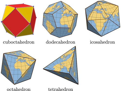
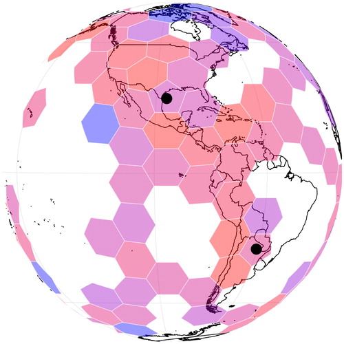
Figure 2. A hexagonal tiling of the Earth based on an icosahedron. Pentagons are marked with black dots. Image produced with dggridR (Barnes 2017), an R package for manipulating discrete global grids.

Hexagonal cells in particular have several convenient properties. All hexagonal cells on a face share a common orientation (as opposed to triangles) and always meet neighbouring cells across edges rather than points (as opposed to both triangles and diamonds), which is convenient for modeling. Hexagonal cells require 13.4% fewer samples to reconstruct certain classes of signals (Mersereau 1979). While a number of other advantages of hexagonal cells are reviewed in He and Jia (2005), the utility of hexagons can be intuited from the fact that they are the basis of the human visual system (Sawides, Castro, and Burns 2017) and the brain's navigation system (Hafting et al. 2005).

Discrete global grids are useful for spatial statistics and have exceptionally low areal and angular distortion as compared to other projections (Snyder 1992; Kimerling et al. 1999; White et al. 1998; Sahr, White, and Kimerling 2003; Gregory et al. 2008). In practice, they have been used for discretizing atmospheric dynamics (Thuburn 1997), ecological observation (Birch, Oom, and Beecham 2007), studying long-range animal migration (Kranstauber et al. 2015), modeling tidal waves (Lin et al. 2018), solving the shallow-water equation (Heikes and Randall 1995a, 1995b), analyzing remote sensing data (Romanov and Khvostov 2018), and for spatial binning by the Uber ridesharing company (Uber Technologies Inc 2018). They have also been proposed as a basis for global digital elevation models (Schumann and Bates 2018).

The mathematical transforms from latitude-longitude to discrete global grid cell indices involve numerous trigonometric calculations and may include iterative methods (Gray 1995; Crider 2008). In the past, such calculations were prohibitively slow; however, recent increases in CPU speed as well as the ability to offload repetitive calculations on large datasets to GPUs has largely overcome this hurdle. Additionally, algorithmic developments such as improved indexing schemes mean that for basic operations such as finding parent, child, and neighbour cells it is now possible to avoid many of these calculations altogether (Lee and Samet 1998; Sahr 2008; Ben et al. 2018; Mocnik 2018; Zhou et al. 2018). Collectively, this is leading to wider usage and standardization efforts (Open Geospatial Consortium 2017).

Unfortunately, discrete global grids are not with issues. For instance, at any resolution a hexagonally-tiled icosahedron will have exactly twelve pentagons, each of which is $5/6$ the size of the hexagons (Kimerling et al. 1999). These sorts of singularities appear at the vertices of all polyhedra and may break important geometric or topologic assumptions made in code or statistical analyses. Figure 2 demonstrates this with a toy example in which the number of earthquakes over a time period are binned and polygonal cells are indicated. Notice that these cells overlap landmasses; this may be undesirable depending on the analysis being performed. Additionally, for any cell geometry, the areal or angular distortion of the cells comprising a grid, though lower than traditional projections, is still a function of their location on a polyhedron's face (White et al. 1998; Kimerling et al. 1999; Gregory et al. 2008).

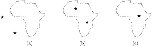
Choosing an orientation which minimizes such effects is a nonconvex optimization problem. Here, I solve this problem for several common polyhedra for several common scenarios depicted in Figure 3 by finding orientations which: (a) Maximize the average distance of all vertices from land; this is useful for applications considering only landmasses. (b) Maximize the average distance of all vertices from water; this is useful for applications considering only oceans. (c) Maximize a single vertex's distance from a coastline; this yields the Poles of Inaccessibility (see below) and is useful for ensuring that a single landmass or ocean of interest has a single singularity near its center; this can be used in place of a polar projection. I also identify orientations which minimize and maximize the overlap of the polyhedron's edges with landmasses; this configuration is useful for minimizing distortion within landmasses or oceans. In addition, I find the orientations which maximize and minimize the number of vertices intersecting landmasses.

Figure 3. Conceptual diagram of some quantities being optimized. See text for further details.

The orientations in the foregoing list will not be suitable for all studies using discrete global grids; however, the source code associated with this paper can be used to generate customized configurations.

1.2. Cartography

In addition to their general applicability to any study using discrete global grids, finding these orientations makes a contribution to cartography. Buckminster Fuller's Dymaxion map is based on an unfolding of the triangular faces of an icosahedron. I have found no evidence that the orientation of Fuller's icosahedron is known to optimize any particular quantity, though Fuller's orientation is claimed to be the only one known for which no vertices fall on land (Sahr 2015). Several tables of coordinates for the vertices of Fuller's orientation exist, but there are differences between the tables as well as internal inconsistencies within some of the tables themselves (Gray 2015).

van Wijk (2008) presents an optimized orientation of an unfolded icosahedron. However, the optimization only minimizes the length of land cut by an unfolded edge of the icosahedron, rather than the total length of land intersecting the icosahedron's edges. That is, it is only suitable for flat maps meant for visual display.

This study finds self-consistent coordinates for Fuller's orientation, as optimized for a known quantity. It also provides an edge-overlap minimizing orientation.

1.3. Poles of Inaccessibility

Finding orientations which maximize the distance of a single vertex from a coastline corresponds to the problem of finding the Poles of Inaccessibility. If the point of a polyhedron is located at such a pole, then the distance of one of its vertices from a coastline is at an extrema and any rotation about this vertex will have this same property. Poles of Inaccessibility, especially the Arctic, Antarctic, Eurasian, and Oceanic poles, have long drawn explorers, often at great personal expense and risk. For this reason, determining their locations accurately is important, though there has been limited work on this.

Garcia-Castellanos and Lombardo (2007) present a method of finding poles by adaptively refining a rectangular grid of test points to zoom in on a pole; however, they perform their calculations assuming a spherical Earth and so generate incorrect values for all poles, though their values are often close to the ones I find and usually within uncertainties induced by coastline data. Martinez (2012) refined the Garcia-Castellanos and Lombardo (2007) method, but did not calculate the locations of Poles. Rees et al. (2014) utilized the Garcia-Castellanos and Lombardo (2007) method, though with ellipsoidal calculations, to find the Arctic Pole. Frączek and Kneller (2015) used converging isolines on a planar projection of the areas in question to find Poles; however, the choice of a planar projection was a poor one and leads to differences of many kilometers versus all other studies. A list of the Poles of Inaccessibility as found here is given in Table 3.

2. Methods

2.1. Outline

Finding suitable orientations of polyhedra for discrete global grids is an optimization problem whose objective is a function of the distance of coastlines to the polyhedras' vertices and edges. The shape of Earth's coastlines implies that this problem is nonconvex (Figure 5). To solve the problem, I use a hillclimbing algorithm with simulated annealing, as detailed below.

The methods described below will exhaustively generate all the possible orientations for each of several polyhedra. This is done at a coarse resolution using elliptical calculations. Duplicate orientations will be searched for and removed. Each remaining member of this sparsely-sampled orientation space will then used as a starting point for a hillclimbing algorithm which finds optimal orientations given some criteria of interest. Several polyhedra are considered here (Figure 1): the cuboctahedron, the regular dodecahedron, the regular icosahedron, the regular octahedron, and the regular tetrahedron. Since textual descriptions may be insufficient to recreate the algorithm, I provide source code on Github at https://github.com/r-barnes/Barnes2017-DggBestOrientations. Various software packages were used in the analysis (Barnes 2017; Becker et al. 2018; McIlroy et al. 2018; Wickham 2016; Wickham et al. 2018).

2.2. Orientating polyhedra

The first step is to develop a method for orientating polyhedra. The orientation of a polyhedron can be described by three parameters: the latitude λ and longitude φ of one of its vertices (henceforth, the ‘primary vertex’) with respect to a fixed coordinate system along with the rotation θ of the other vertices about a vector from the origin to the primary vertex, where latitude $\lambda \in [-{90}^{\circ },{90}^{\circ }]$, longitude $\phi \in [-{180}^{\circ },{180}^{\circ })$, and rotation $\theta =[0^{\circ },{360}^{\circ })$.

Table 1 lists the nominal vertex coordinates of the polyhedra. Each polyhedron was rotated from this default orientation to one in which its primary vertex was aligned with $\lambda ={90}^{\circ },\phi =0$. To do this, the 3-space coordinates of the polyhedra were normalized. The vector $\overrightarrow{P}$ connecting the origin to the primary vertex was then crossed with the $(0,0,1)$ polar vector ($\overrightarrow{P}\times (0,0,1)$) to generate a vector $\overrightarrow{r}$ about which the polyhedra needed to be rotated to obtain a polar configuration. Following Glassner (1990, p. 466), the quantities $c=\overrightarrow{P}\cdot (0,0,1)$, $s=\sqrt{1-c^2}$, t = 1−c were defined and the rotation matrix:(1) $\mathbf{R}=\left[\begin{array}{ccc}t{x}^2+c& txy+sz& txz-sy\\ txy-sz& t{y}^2+c& tyz+sx\\ txz+sy& tyz-sx& t{z}^2+c\end{array}\right]$(1) generated, where x,y,z were drawn from $\overrightarrow{r}$. An arbitrary vector $\overrightarrow{v}$'s coordinates in the polar configuration were then ${\overrightarrow{v}}^{\prime }=\mathbf{R}\overrightarrow{v}$.

Table 1. Nominal vertex coordinates of the polyhedra considered in this paper.

Polyhedron	Primary Vertex	Vertices
Regular Icosahedron	$(0,{90}^{\circ })$	$(0,\pm {90}^{\circ }),(36n^{\circ },-1^n\arctan (\frac{1}{2}\left)\right)\mathrm{\forall }n$
Regular Dodecahedron	$(1,1,1)$	$(\pm 1,\pm 1,\pm 1)$, $(0,\pm \phi ,\pm {\phi }^{-1})$, $(\pm {\phi }^{-1},0,\pm \phi )$, $(\pm \phi ,\pm {\phi }^{-1},0)$
Regular Tetrahedron	$(1,0,-1/\sqrt{2})$	$(\pm 1,0,-1/\sqrt{2})$, $(0,\pm 1,1/\sqrt{2})$
Regular Octahedron	$(1,0,0)$	$(\pm 1,0,0)$, $(0,\pm 1,0)$, $(0,0,\pm 1)$
Cuboctahedron	$(1,1,0)$	$(\pm 1,\pm 1,0)$, $(\pm 1,0,\pm 1)$, $(0,\pm 1,\pm 1)$

Notes: Vertices are generated by taking all permutations of the ± signs and all unique values of n. The symbol φ denotes the golden ratio: $\frac{1+\sqrt{5}}{2}$.

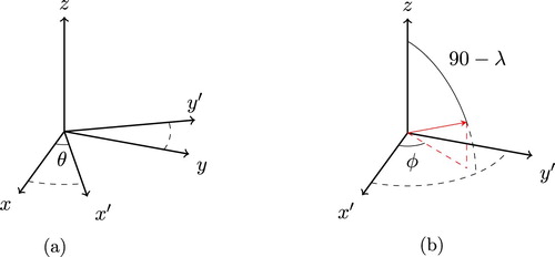
Once the polyhedra were in the normalized polar configuration described above, they could be rotated to any orientation $(\lambda ,\phi ,\theta )$ by first rotating all points by an angle θ about the z-axis (Figure 4(a)). A unit vector to $(\lambda ,\phi )$ could then be calculated and the matrix from Equation 1(1) $\mathbf{R}=\left[\begin{array}{ccc}t{x}^2+c& txy+sz& txz-sy\\ txy-sz& t{y}^2+c& tyz+sx\\ txz+sy& tyz-sx& t{z}^2+c\end{array}\right]$(1) generated (Figure 4(b)). The polyhedra could then be rotated so that their polar vertex was coincident with the point described by $(\lambda ,\phi )$. Note that θ and φ are not redundant: the former changes the locations of all a polyhedron's vertices only about the z axis while the latter changes their location with respect to an arbitrary rotation vector.

Figure 4. Polyhedral rotations. Note that θ and φ are not redundant. (a) Rotation about the polar vector (b) Rotation to a new polar vector.

2.3. Enumerating polyhedral orientations

The second step was to generate a list of initial orientations. To do so, the polar vertex was rotated to a series of positions generated by a Fibonacci spiral wrapped about a sphere (Marques, Bouville, and Bouatouch 2013, Equation 4). This construction produces a set of orientations which are distributed more or less evenly across the Earth with a separation of approximately 100 km. As detailed below, as orientations were generated, those with either no vertices intersecting a landmass or with many vertices intersecting landmasses were retained. Orientations which were close to each other were discarded.

2.4. Finding landmass intersections

To determine how many vertices of an orientation intersected a landmass, Web-Mercator projected landmass polygons were acquired from OpenStreetMap (OpenStreetMap contributors 2017; Topf and Hormann 2017a). Conveniently, in this dataset large landmasses were subdivided into smaller polygons. The polygons' bounding boxes were pack-loaded into a Boost R-Tree (Wulkiewicz 2017) and those which were perfect rectangles were noted as such. This enabled quick point-in-box checks for the projected vertices. When these checks indicated the possibility of landmass intersection for a non-rectangular region, a more expensive point-in-polygon check was performed using a method elaborated by Franklin (1970). Orientations with either zero or many landmass intersections were retained.

2.5. Search space pruning

Detecting nearby orientations was necessary to reduce the search space and the number of results found by the optimization procedure. To do so, orientations' vertices were projected into Cartesian 3-space and placed into a nanoflann (Blanco 2014) kd-tree. For a given orientation O, neighbouring orientations could be found by querying the kd-tree for a list of vertices nearby to each vertex of O. If another orientation $O^{\prime }$ appeared in each list, then each of its vertices was nearby to one of O's vertices, implying that $O^{\prime }$ was nearby to O and allowing one of the two to be discarded.

2.6. Finding optimal orientations

The third step was to optimize the orientations. To do so, for a given polyhedron and orientation, the distances of the polyhedrons vertices to the nearest coastline were determined, as described below. If a vertex fell within a landmass its distance to a coastline was taken as negative; otherwise, the distance was taken as positive.

Orientations were optimized for several quantities. (a) Orientations which maximize some vertex's distance from a coastline (the Poles of Inaccessibility); these could be found efficiently by optimizing for a single vertec and ignore the rest. (b) Orientations which minimize and maximize the average distance across all vertices from coastlines; orientations where vertices are far from the ocean or far from land, respectively. (c) Orientations which minimize and maximize the overlap of the polyhedron's edges with landmasses.

To determine the vertices' distance from land, WGS84 landmass polygons were acquired from OpenStreetMap (OpenStreetMap contributors 2017; Topf and Hormann 2017b). Since calculating the distance between vertices and landmass line segments would have been prohibitively slow, interpolation was performed to ensure that no segment of coastline exceeded 500 m in length. Segments exceeding this threshold were subdivided by inserting points at 500 m intervals along a great circle arc connecting the segment's endpoints. Using the great circle approximation for interpolation is permissible because the distances involved were small: no segment of coastline exceeded more than a few tens of kilometres in length.

All the interpolated points and the endpoints of the original segments were then projected into Cartesian 3-space using geographiclib (Karney 2017) for ellipsoidal calculations and indexed using a nanoflann (Blanco 2014) kd-tree for quick nearest-neighbour lookups. Once a vertex's nearest neighbour was identified, great ellipse distances were calculated using geographiclib's distance routines. For each orientation, the minimum, maximum, and average distances of its vertices from coastlines were retained.

2.7. Hillclimbing

To find optimal orientations, each of the orientations generated by the Fibonacci spiral (§2.3) was used as the initial value of a simulated annealing hillclimbing algorithm (Russell and Norvig 2002, §4.3; Skiena 2012, §7.5.2). For a given orientation, the hillclimbing algorithm chose at random one of $\lambda ,\phi ,\theta$ and added to it a value δ drawn from a normal distribution with zero mean and and some standard deviation on the order of a half-degree. If the modified orientation was better than the original, it was retained and modified itself; otherwise, another attempt at improvement was made using a different modification. After a threshold number of failures, the algorithm terminated. To obtain high-precision estimates of the optimal orientations the standard deviation of δ was annealed; that is, its value was reduced in several stages. Simultaneously, the number of failed attempts at improvement was increased.

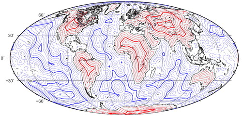
For each initial value, the hillclimbing algorithm was run several times. Using several initial values, repeated runs, and annealing all help hillclimbing algorithms to avoid local optima and find global optima (Russell and Norvig 2002, §4.3; Skiena 2012, §7.5.2). In addition, as shown in Figure 5, the search space was characterized by smooth isolines and broad basins of attraction, which meant the hillclimber had a favourable working environment.

Figure 5. Isolines of distance from shorelines. Note the smoothness of the isolines and the broad basins of attraction: this is a good environment for hillclimbing algorithms. Image adapted from Gaianauta and Wikipedia Contributors (2017) and generated using the method described by Garcia-Castellanos and Lombardo (2007).

2.8. Poles of Inaccessibility

The location of the Poles of Inaccessibility is a function of the data used to constrain them; therefore, for finding the Poles of Inaccessibility several datasets were used: the OpenStreetMap data described above as well as the full-resolution versions of the L1 (land-ocean divide), L5 (Antarctic ice), and L6 (Antarctic grounding line) subsets of the Global Self-consistent, Hierarchical, High-resolution Geography (GSHHG)'s coastline data (Wessel and Smith 2016).

For each dataset and pole, a similar optimization process to that described above was repeated. Hillclimbing was begun at the Fibonacci spiral points discussed earlier, as well as at all Poles identified by previous authors.

The extent of the polyhedron's edges which overlap landmasses is also of interest. This value was estimated by generating sample points every 1 km along great circles connecting a polyhedron's vertices. The point-in-landmass check described above was then applied to each point and the number of points within a landmass taken as an estimate of the overlap.

2.9. Precision

The algorithm's precision is acceptable. Separate runs of the hillclimbing procedure usually resulted in values within less than 10 m of each other. For points within 5000 km of the Earth's surface, geographiclib's error is bounded by 7 nm for the WGS84 ellipsoid (Karney 2017). The data sources are also fairly accurate. 90% of identifiable coastal features in the GSHHG data are stated to be within 500 m of their true locations (Wessel and Smith 2016). An analysis of OpenStreetMap's coastline data shows that many of the line segments forming the coasts have characteristics suggesting accuracy (Hormann 2013).

2.10. Compute requirements

Computation and data utilized single nodes on XSEDE's Comet supercomputer (Towns et al. 2014) with 128 GB RAM and Intel Xeon E5-2680v3 CPUs. Running the algorithm consumed about 3.2 GB of RAM, most of which was needed to store coastline data and spatial indices. Using less detailed datasets or reducing the number of interpolated coastline points could reduce this value significantly. Finding all the Poles of Inaccessibility took about 30 s, finding extreme values for orientations without considering edge overlaps took about 270–390 s depending on the polyhedron. Minimizing and maximizing edge overlaps took about 10.5 hrs; this time could be reduced by using greater parallelism to perform point-in-landmass checks or fewer great arc points to estimate edge overlap. However, in most applications, a discrete global grid will be generated and orientated only once, so these time costs are likely acceptable.

3. Results & discussion

While the tables included here specify only the orientation of each polyhedron for each objective, the full vertex coordinates of the top one hundred orientations for each objective are available in a dataset on Zenodo (Barnes 2019).

3.1. Polyhedral orientations

The optimal orientations found by the methods described above are listed in Table 2 and shown in Figure 6. These orientations offer advantages over those previously known by allowing a practitioner to selectively minimize the effects of distortion in modeling and statistical calculations. Where these orientations are not suitable, the provided code can be used to generate new ones.

Figure 6. Vertices of the Optimal Icosahedral Orientations. Purple squares represent the orientation which minimizes edge overlap with landmasses; green triangles maximize edge overlap. Blue diamonds stars represent the orientation in which vertices are, on average, farthest from water; red circles represent the orientation in which vertices are, on average, farthest from land.

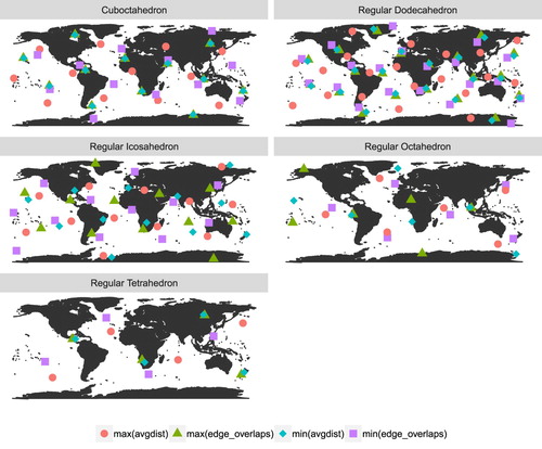
Table 2. Optimal orientations for various quantities.

Polyhedron	∩	Objective	Value (km)	λ	φ	θ
Cuboctahedron	0	max(avg dist)	735.01	38.9689	138.8750	10.6348
Cuboctahedron	9	max(avg dist)	−4.04	51.3955	119.7020	38.4839
Cuboctahedron	0	min(avg dist)	205.55	39.6608	−123.7870	36.8049
Cuboctahedron	9	min(avg dist)	−26.79	52.0223	121.4800	38.9133
Cuboctahedron	0	max(edge)	2460.00	18.8825	105.7470	118.3770
Cuboctahedron	9	max(edge)	2800.00	51.5696	120.4260	38.7461
Cuboctahedron	0	min(edge)	1368.00	72.9324	123.2670	157.9570
Cuboctahedron	9	min(edge)	2632.00	51.5923	119.8290	37.6189
Regular Dodecahedron	12	max(avg dist)	298.92	72.2229	−79.1023	31.0049
Regular Dodecahedron	12	min(avg dist)	−37.91	61.9328	121.9160	65.9673
Regular Dodecahedron	12	max(edge)	2438.00	16.7750	36.9887	33.0034
Regular Dodecahedron	12	min(edge)	2025.00	14.1091	34.6717	19.9835
Regular Icosahedron	0	max(avg dist)	717.62	25.4981	−139.4880	58.2846
Regular Icosahedron	8	max(avg dist)	407.80	21.8598	−14.1591	47.9955
Regular Icosahedron	0	min(avg dist)	223.73	24.9672	67.4845	57.7353
Regular Icosahedron	8	min(avg dist)	44.18	34.5965	−85.5585	34.8110
Regular Icosahedron	0	max(edge)	3147.00	55.0965	140.7330	15.5157
Regular Icosahedron	8	max(edge)	3576.00	79.1494	−54.0237	49.0449
Regular Icosahedron	0	min(edge)	2456.00	18.9602	−61.1569	21.7798
Regular Icosahedron	8	min(edge)	3007.00	37.3477	−85.0918	33.5892
Regular Octahedron	0	max(avg dist)	603.07	54.6526	−37.6691	61.7792
Regular Octahedron	0	min(avg dist)	18.11	6.5108	99.6481	27.2856
Regular Octahedron	0	max(edge)	2115.00	5.4642	−140.9980	2.2740
Regular Octahedron	6	max(edge)	2364.00	70.1654	−152.9320	11.0783
Regular Octahedron	0	min(edge)	631.00	43.7180	154.1320	72.1882
Regular Octahedron	6	min(edge)	2225.00	70.4859	−158.0970	10.7513
Regular Tetrahedron	0	max(avg dist)	500.94	−20.1978	71.8464	79.3600
Regular Tetrahedron	0	min(avg dist)	3.30	64.3874	−64.6626	97.0248
Regular Tetrahedron	4	min(avg dist)	−193.32	14.4545	−84.0842	104.7930
Regular Tetrahedron	4	min(avg dist)	−9.80	55.8814	−88.5392	44.2746
Regular Tetrahedron	0	max(edge)	1654.00	36.7333	52.4700	26.8652
Regular Tetrahedron	4	max(edge)	1662.00	−44.7858	167.9140	18.9960
Regular Tetrahedron	0	min(edge)	408.00	49.8592	−37.3255	5.9246
Regular Tetrahedron	4	min(edge)	1088.00	−15.4571	47.9196	87.5066

Notes: Orientations are given in degrees by the latitude λ and longitude φ of a polar vertex along with the rotation θ of the other vertices about a vector connecting the origin to the polar vertex, as described in the text. The ∩ number indicates the number of the orientation's vertices which intersected land. Objective is the value which was optimized: either the ‘edge’, the kilometres of edges overlapping land, or ‘avg dist’, the average distance of all the polyhedron's points to a coastline. Distances from vertices intersecting a landmass to its coastline are measured in negative kilometres, so ‘min(avg dist)’ places points within landmasses and ‘max(avg dist)’ places points in oceans. All values were calculated using the OpenStreetMap WGS84 data (Topf and Hormann 2017b).

Table 3. Poles of Inaccesibility.

Region	Dataset	Longitude	Latitude	Distance	Stated
		(deg. E)	(deg. N)	(km)	(km)
Africa	Garcia-Castellanos and Lombardo (2007)	26.17	5.65	1812.4620	1814
Africa	GSHHG	26.1533	5.6413	1814.5158
Africa	OpenStreetMap	26.1295	5.6589	1815.4150
Antarctica	Soviet Station Loc	54.9666	−82.1	721.7009
Antarctica	GSHHG L1+L5	103.6340	−78.2633	1273.2928
Antarctica	GSHHG L1+L6	105.3855	−77.3963	1136.2129
Antarctica	OpenStreetMap	104.1178	−78.2582	1271.1539
Arctic Pole	Rees et al. (2014)	176.149	85.802	1007.6039	1008
Arctic Pole	GSHHG	176.1423	85.8015	1007.6777
Arctic Pole	OpenStreetMap	176.2386	85.7911	1008.9112
Atlantic Ocean	GSHHG	−43.3728	24.1923	2033.5187
Atlantic Ocean	OpenStreetMap	−43.3704	24.1851	2033.8849
Australia	Garcia-Castellanos and Lombardo (2007)	132.27	−23.17	915.6601	928
Australia	GSHHG	132.2759	−23.1732	925.4459
Australia	OpenStreetMap	132.1727	−23.1948	921.9290
Eurasia 1	Garcia-Castellanos and Lombardo (2007)	88.14	45.28	2508.0536	2514
Eurasia 2	Garcia-Castellanos and Lombardo (2007)	82.19	44.29	2505.4197	2510
Eurasia 1	GSHHG	88.2483	45.3413	2513.9415
Eurasia 2	GSHHG	82.1144	44.3184	2509.9685
Eurasia 1	OpenStreetMap	88.3172	45.4435	2509.9536
Eurasia 2	OpenStreetMap	83.9694	44.6740	2505.2134
Great Britain	Garcia-Castellanos and Lombardo (2007)	−1.56	52.65	107.7333	108
Great Britain	OpenStreetMap	−0.9640	52.0141	114.4462
Great Britain	GSHHG	−1.5641	52.6552	108.0925
Greenland	Garcia-Castellanos and Lombardo (2007)	−41.0	76.50	471.2712	469
Greenland	GSHHG	−40.4239	75.9660	471.9905
Greenland	OpenStreetMap	−40.3902	76.0305	474.2257
Indian Ocean	GSHHG L1	100.0547	−47.7347	1943.3848
Indian Ocean	OpenStreetMap	99.9677	−47.6319	1940.8913
Madagascar	Garcia-Castellanos and Lombardo (2007)	46.67	−18.33	258.7060	260
Madagascar	OpenStreetMap	46.7003	−18.2645	264.0657
Madagascar	GSHHG	46.6663	−18.3382	259.5957
North America	Garcia-Castellanos and Lombardo (2007)	−101.97	43.46	1629.7740	1639
North America	GSHHG	−102.0111	43.3764	1639.6549
North America	OpenStreetMap	−102.0101	43.4370	1643.7562
Pacific Ocean (Point Nemo)	GSHHG	−123.4345	−49.0273	2704.7991
Pacific Ocean (Point Nemo)	OpenStreetMap	−123.3920	−49.0031	2701.1721
Pacific Ocean (Point Nemo)	Garcia-Castellanos and Lombardo (2007)	−123.45	−48.89	2689.4857	2690
South America	Garcia-Castellanos and Lombardo (2007)	−56.85	−14.05	1449.9471	1517
South America 1	GSHHG	−56.9922	−14.3902	1490.5321
South America 2	GSHHG	−65.5487	−5.0537	1476.4901
South America 1	OpenStreetMap	−63.1885	−6.3248	1511.6636
South America 2	OpenStreetMap	−59.2126	−10.7342	1467.2206

Notes: If Dataset lists GSHHG or OpenStreetMap, then the calculation was performed in this study; otherwise, the value is drawn from the source provided. All locations are listed for WGS84. Distance is distance with respect to the GSHHG or OpenStreetMap coastline. For values drawn from other studies, the distance has been recalculated for the GSHHG coastline (Wessel and Smith 2016) used in this study. Stated is the distance as stated in the original study. The difference between Distance and Stated is due to this study's improved techniques and, possibly, updated coastline data. Results from Frączek and Kneller (2015) are omitted due to their low accuracy.

For each polyhedron, the orientations which maximized and minimized the number of vertices intersecting landmasses also turned out to maximize or minimize other quantities of interest. Thus, if this is the only value that needs to be optimized for an application, one of several entries can be chosen from Table 2.

Until now, Fuller's was the only known icosahedral orientation with no vertices intersecting land. In contrast, four such distinct optimal orientations are listed in Table 2. Many others which were suboptimal are included in the Zenodo dataset. Of the optimal icosahedral orientations, Fuller's most closely resembles my orientation which places no vertices on land while minimizing edge overlap with landmasses. This makes a certain sense, as such an orientation would be one of the easiest to find without the computational techniques used here.

3.2. Poles of Inaccessibility

In some cases, my results for the Poles of Inaccessibility agree with previous authors' to within a half-kilometre, lending credence to both methods. In other cases, I am able to improve on previous results by several kilometres due to the use of ellipsoidal calculations, improved optimization techniques, and better coastline data. The results are shown in Table 3.

The difference between older values and those calculated in this study is most dramatic for Point Nemo, the Oceanic Pole of Inaccessibility, which I find to be 15 km from the site originally calculated by Lukatela (2004). Measuring the distance of the coordinates specified by Lukatela (2004) to the coastlines used in this study gives a distance within 0.5 km of Lukatela (2004)'s. This strongly suggests that the improvement is due not to differences in data, but to improved optimization techniques. The new location of Point Nemo is similar across the datasets used, including the GSHHG L1, L1+L5, and L1+L6 data; that is, the location is not a function of the grounding line of the Antarctic ice cap.

The data sources used suggest two Eurasian Poles, in agreement with Garcia-Castellanos and Lombardo (2007). South America is found to have one pole, but, 1400 km away, there is a second contender whose distance from the sea is within 14 km of the first. The location of the Arctic Pole agrees with a recent calculation (Rees et al. 2014).

The Antarctic Pole's location is much debated, due primarily to whether or not coastal ice shelves are included and where grounding lines are believed to lie. I use several coastlines (see Table 3) and find locations that differ from others previously generated. However, given the up-to-date data used and the accuracy of the method, these are likely the most accurate locations yet calculated.

4. Conclusions

The foregoing describes a method for optimally orientating the polyhedra which underlie discrete global grids. This will allow researchers to minimize distortion and nonconformities within areas of interest. The method was applied to find several optimal orientations for several polyhedra. The orientations found are superior to those used as defaults in existing software in that they minimize or maximize quantities which may affect the statistical accuracy of calculations.

More concretely, the method provides a disciplined way of orientating polyhedra so that their singularities (such as the twelve pentagons in the icosahedral hexagonal discrete global grid) are located away from study areas. This can eliminate special cases in GIS and modeling software, leading to reduced run-times. Though discrete global grids already have low distortion, the method provides a way to reduce this further by locating vertices and edges nearer or farther from study regions (depending on the use case). Pre-calculated values for some common scenarios are provided.

This paper makes a contribution to cartography by providing a set of self-consistent coordinates for Buckminster Fuller's Dymaxion map and identifying Fuller's orientation as an approximation of the optimal orientation found here which places no vertices on land while minimizing edge overlap with landmasses.

Several of the orientations correspond to improved values for the Poles of Inaccessibility, mostly notably for the Oceanic Pole of Inaccessibility (Point Nemo), which is found to be 15 km farther from land than previously known.

Acknowledgments

Kelly Kochasnski, Yakov Berchenko Kogan, and Allison Jonjak provided useful discussion. Coastline data is copyrighted to ‘OpenStreetMap contributors’ and available from https://www.openstreetmap.org. Adam Clark furnished the laptop on which development work was done. I have no conflicts of interest to declare with regards to this work.

Disclosure statement

No potential conflict of interest was reported by the author.

Correction Statement

This article has been republished with minor changes. These changes do not impact the academic content of the article.

Additional information

Funding

This work was supported by the Department of Energy Computational Science Graduate Fellowship (Krell Institute) under grant DE-FG02-97ER25308, the Gordon and Betty Moore Foundation through Grant GBMF3834, and by the Alfred P. Sloan Foundation through Grant 2013-10-27 to the University of California, Berkeley. Computation and data utilized XSEDE’s Comet supercomputer (Towns et al. 2014), which is supported by the National Science Foundation (Grant No. ACI-1053575). In-kind support was provided by the Carnes and Ormac families, as well as Michelle Oliver and the Los Alamos Public Library.

References

- Barnes, Richard. 2017. “dggridR: Discrete Global Grids for R.” R package version 1.0.1. Available from: https://CRAN.R-project.org/package=dggridR.
- Barnes, Richard. 2019. “Source Code: Optimal Orientations of Discrete Global Grids.” Zenodo. doi:10.5281/zenodo.2551665.
- Becker, Richard, Allan Wilks, Ray Brownrigg, Thomas Nika, and Alex Deckmyn. 2018. “Maps: Draw Geographical Maps.” R package version 3.3.0, https://CRAN.R-project.org/package=maps.
- Ben, Jin, Ya Lu Li, Cheng Hu Zhou, Rui Wang, and Ling Yu Du. 2018. “Algebraic Encoding Scheme for Aperture 3 Hexagonal Discrete Global Grid System.” Science China Earth Sciences 61 (2): 215–227. doi: 10.1007/s11430-017-9111-y
- Birch, Colin, Sander P. Oom, and Jonathan Beecham. 2007. “Rectangular and Hexagonal Grids Used for Observation, Experiment and Simulation in Ecology.” Ecological Modelling 206 (3–4): 347–359. doi:10.1016/j.ecolmodel.2007.03.041.
- Blanco, Jose Luis. 2014. “nanoflann: A C++ Header-Only Fork of FLANN, A Library for Nearest Neighbor (NN) With KD-trees.” Version 1.2.3, https://github.com/jlblancoc/nanoflann.
- Crider, John. 2008. “Exact Equations for Fuller's Map Projection and Inverse.” Cartographica: The International Journal for Geographic Information and Geovisualization 43 (1): 67–72. doi:10.3138/carto.43.1.67.
- Open Geospatial Consortium. 2017. “Discrete Global Grid Systems Abstract Specification.” http://www.opengis.net/doc/AS/dggs/1.0.
- Gaianauta and Wikipedia Contributors. 2017. “Distancia a la costa.” Accessed on 31 July 2017. https://commons.wikimedia.org/wiki/File:Distancia_a_la_costa.png.
- Franklin, W. Randolph. 1970. “PNPOLY – Point Inclusion in Polygon Test.” Accessed on 4 May 2017. https://wrf.ecse.rpi.edu//Research/Short_Notes/pnpoly.html.
- Frączek, Witold, and Lenny Kneller. 2015. “Poles of Inaccessibility – The Remotest Places on Earth.” Accessed on 29 March 2018. https://apl.maps.arcgis.com/apps/MapJournal/index.html?appid=ce19bec7a3c541d0b95c449df9bb8eb5.
- Garcia-Castellanos, Daniel, and Umberto Lombardo. 2007. “Poles of Inaccessibility: A Calculation Algorithm for the Remotest Places on Earth.” Scottish Geographical Journal 123 (3): 227–233. doi:10.1080/14702540801897809.
- Glassner, Andrew S., ed. 1990. Graphics Gems. San Diego, CA: Academic Press Professional.
- Gray, Robert. 1995. “Exact Transformation Equations for Fuller's World Map.” Cartographica: The International Journal for Geographic Information and Geovisualization 32 (3): 17–25. doi:10.3138/1677-3273-Q862-1885.
- Gray, Robert. 2015. “Fuller's World Map: Coordinates.” Accessed on 27 March 2018. http://www.rwgrayprojects.com/rbfnotes/maps/graymap4.html.
- Gregory, Matthew, A. Jon Kimerling, Denis White, and Kevin Sahr. 2008. “A Comparison of Intercell Metrics on Discrete Global Grid Systems.” Computers, Environment and Urban Systems 32 (3): 188–203. doi:10.1016/j.compenvurbsys.2007.11.003.
- Uber Technologies Inc. 2018. “H3: A Hexagonal Hierarchical Geospatial Indexing System.” Accessed on 29 March 2018. https://github.com/uber/h3.
- Hafting, Torkel, Marianne Fyhn, Sturla Molden, May-Britt Moser, and Edvard I. Moser. 2005. “Microstructure of a Spatial Map in the Entorhinal Cortex.” Nature 436 (7052): 801. doi:10.1038/nature03721.
- He, Xiangjian, and Wenjing Jia. 2005. “Hexagonal Structure for Intelligent Vision.” In 2005 International Conference on Information and Communication Technologies, Aug., 52–64. doi:10.1109/ICICT.2005.1598543.
- Heikes, Ross, and David Randall. 1995a. “Numerical Integration of the Shallow-Water Equations on a Twisted Icosahedral Grid. Part II: A Detailed Description of the Grid and an Analysis of Numerical Accuracy.” Monthly Weather Review 123: 1881–1887. doi: 10.1175/1520-0493(1995)123<1881:NIOTSW>2.0.CO;2
- Heikes, Ross, and David A. Randall. 1995b. “Numerical Integration of the Shallow-water Equations on a Twisted Icosahedral Grid. Part I: Basic Design and Results of Tests.” Monthly Weather Review 123 (6): 1862–1880. doi: 10.1175/1520-0493(1995)123<1862:NIOTSW>2.0.CO;2
- Hormann, Christoph. 2013. “Assessing the OpenStreetMap Coastline Data Quality.” Accessed on 29 March 2018, 4, http://www.imagico.de/map/coastline_quality_en.php.
- Karney, C. F. F. 2017. “GeographicLib, Version 1.48 (April, 2017).” https://geographiclib.sourceforge.io/1.48.
- Kimerling, Jon A., Kevin Sahr, Denis White, and Lian Song. 1999. “Comparing Geometrical Properties of Global Grids.” Cartography and Geographic Information Science 26 (4): 271–288. doi:10.1559/152304099782294186.
- Kranstauber, B., R. Weinzierl, M. Wikelski, and K. Safi. 2015. “Global Aerial Flyways Allow Efficient Travelling.” Ecology Letters 18 (12): 1338–1345. doi:10.1111/ele.12528.
- Lee, Michael, and Hanan Samet. 1998. “Traversing the Triangle Elements of an Icosahedral Spherical Representation in Constant-Time.” In Proc. 8th Intl. Symp. on Spatial Data Handling, Vancouver, Canada, Jul., 22–33. Accessed 23 July 2017. https://www.cs.umd.edu/hjs/pubs/leesdh98short.pdf.
- Lin, Bingxian, Liangchen Zhou, Depeng Xu, A-Xing Zhu, and Guonian Lu. 2018. “A Discrete Global Grid System for Earth System Modeling.” International Journal of Geographical Information Science32 (4): 711–737. https://doi.org/10.1080/13658816.2017.1391389.
- Lukatela, Hrvoje. 2004. “Point Nemo.” Accessed on 29 March 2018. http://www.geocuriosa.com/pointnemo/index.html.
- Marques, Ricardo, Christian Bouville, and Kadi Bouatouch. 2013. “Spherical Fibonacci Point Sets for Illumination Integrals.” In Computer Graphics Forum, Vol. 32, 134–143. Wiley Online Library. doi:10.1111/cgf.12190.
- Martinez, Oscar. 2012. “An Efficient Algorithm to Calculate the Center of the Biggest Inscribed Circle in an Irregular Polygon.” preprint arXiv:1212.3193.
- McIlroy, Doug, Ray Brownrigg, Thomas P. Minka, and Roger Bivand. 2018. “mapproj: Map Projections.” R package version 1.2.6, https://CRAN.R-project.org/package=mapproj.
- Mersereau, R. M. 1979. “The Processing of Hexagonally Sampled Two-dimensional Signals.” Proceedings of the IEEE 67 (6): 930–949. doi:10.1109/PROC.1979.11356.
- Mocnik, Franz-Benjamin. 2018. “A Novel Identifier Scheme for the ISEA Aperture 3 Hexagon Discrete Global Grid System.” Cartography and Geographic Information Science 1–15. doi:10.1080/15230406.2018.1455157.
- OpenStreetMap contributors. 2017. “Planet Dump Retrieved From https://planet.osm.org.” https://www.openstreetmap.org.
- Rees, Gareth, Robert Headland, Ted Scambos, and Terry Haran. 2014. “Finding the Arctic Pole of Inaccessibility.” Polar Record 50 (01): 86–91. doi:10.1017/S003224741300051X.
- Romanov, Andrey, and Ilya Khvostov. 2018. “Emissivity Peculiarities of the Inland Salt Marshes in the South of Western Siberia.” International Journal of Remote Sensing 39 (2): 418–431. doi:10.1080/01431161.2017.1385105.
- Russell, Stuart, and Peter Norvig. 2002. Artificial Intelligence: A Modern Approach. 2nd ed. Upper Saddle River, N.J.: Prentice Hall.
- Sahr, Kevin. 2008. “Location Coding on Icosahedral Aperture 3 Hexagon Discrete Global Grids.” Computers, Environment and Urban Systems 32 (3): 174–187. Accessed 11 July 2016. http://linkinghub.elsevier.com/retrieve/pii/S0198971507000889 doi: 10.1016/j.compenvurbsys.2007.11.005
- Sahr, Kevin. 2015. “R. Buckminster Fuller's Dymaxion Orientation.” Accessed on 27 March 2018. http://webpages.sou.edu/sahrk/dgg/orientation/dymorient.html.
- Sahr, Kevin, Denis White, and A. Jon Kimerling. 2003. “Geodesic Discrete Global Grid Systems.” Cartography and Geographic Information Science 30 (2): 121–134. doi:10.1559/152304003100011090.
- Sawides, Lucie, Alberto de Castro, and Stephen A. Burns. 2017. “The Organization of the Cone Photoreceptor Mosaic Measured in the Living Human Retina.” Vision research 132: 34–44. doi:10.1016/j.visres.2016.06.006.
- Schumann, Guy J.-P., and Paul D. Bates. 2018. “The Need for a High-Accuracy, Open-Access Global DEM.” Frontiers in Earth Science 6: 225. doi:10.3389/feart.2018.00225, https://www.frontiersin.org/article/10.3389/feart.2018.00225.
- Skiena, Steven. 2012. The Algorithm Design Manual. 2nd ed. London: Springer.
- Snyder, John. 1992. “An Equal-Area Map Projection for Polyhedral Globes.” Cartographica: The International Journal for Geographic Information and Geovisualization 29 (1): 10–21. doi:10.3138/27H7-8K88-4882-1752.
- Thuburn, John. 1997. “A PV-based Shallow-Water Model on a Hexagonal-Icosahedral Grid.” Monthly Weather Review 125 (9): 2328–2347. doi:10.1175/1520-0493(1997)125<2328:APBSWM>2.0.CO;2.
- Topf, Jochen, and Christoph Hormann. 2017a. “OpenStreetMap Data: Land Polygons.” Data retrieved from http://openstreetmapdata.com/data/land-polygons; exact file was http://data.openstreetmapdata.com/land-polygons-split-3857.zip entitled “Format: Shapefile, Projection: Mercator, Last update: 2017-04-26 08:54 (Large polygons are split, use for larger zoom levels)”.
- Topf, Jochen, and Christoph Hormann. 2017b. “OpenStreetMap Data: Land Polygons.” Data retrieved from http://openstreetmapdata.com/data/land-polygons; exact file was http://data.openstreetmapdata.com/land-polygons-complete-4326.zip entitled “Format: Shapefile, Projection: WGS84, Last update: 2017-04-26 08:54 (Large polygons not split)”.
- Towns, John, Timothy Cockerill, Maytal Dahan, Ian Foster, Kelly Gaither, Andrew Grimshaw, and Victor Hazlewood, et al. 2014. “XSEDE: Accelerating Scientific Discovery.” Computing in Science & Engineering 16 (5): 62–74. doi:10.1109/MCSE.2014.80.
- van Wijk, Jarke. 2008. “Unfolding the Earth: Myriahedral Projections.” The Cartographic Journal 45 (1): 32–42. doi:10.1179/000870408X276594.
- Wessel, Paul, and Walter H. F. Smith. 2016. “A Global Self-consistent, Hierarchical, High-resolution Geography Database.” v2.3.6, revision 641, released on 17 August 2016. http://www.soest.hawaii.edu/wessel/gshhg/.
- White, Denis, A. Jon Kimerling, Kevin Sahr, and Lian Song. 1998. “Comparing Area and Shape Distortion on Polyhedral-based Recursive Partitions of the Sphere.” International Journal of Geographical Information Science 12 (8): 805–827. doi:10.1080/136588198241518.
- Wickham, Hadley. 2016. ggplot2: Elegant Graphics for Data Analysis. New York: Springer-Verlag.
- Wickham, Hadley, Romain François, Lionel Henry, and Kirill Müller. 2018. “dplyr: A Grammar of Data Manipulation.” R package version 0.7.6, https://CRAN.R-project.org/package=dplyr.
- Wulkiewicz, Adam. 2017. “Boost Geometry Spatial Index.” Version 1.64. http://www.boost.org/doc/libs/1_64_0/libs/geometry/doc/html/geometry/spatial_indexes/introduction.html.
- Zhou, Liangchen, Wenjie Lian, Guonian Lv, A-Xing Zhu, and Bingxian Lin. 2018. “Efficient Encoding and Decoding Algorithm for Triangular Discrete Global Grid Based on Hybrid Transformation Strategy.” Computers, Environment and Urban Systems 68: 110–120. doi:10.1016/j.compenvurbsys.2017.11.005.