An open-source web service for creating quadrilateral grids based on the rHEALPix Discrete Global Grid System

ABSTRACT

The foundation of modern Digital Earth frameworks is the Discrete Global Grid System (DGGS). To standardize the DGGS model, the Open Geospatial Consortium (OGC) recently created the DGGS Abstract Specification, which also aims to increase usability and interoperability between DGGSs. To support these demands and aid future research, open implementations are necessary. However, several OGC conformant DGGSs are not available for researchers to use. This has motivated us to develop an open-source web service that allows users to create quadrilateral grids based on the rHEALPix DGGS. In this paper, we describe the implementation of the web service, including issues and limitations, and demonstrate how discrete global grids and regional grids can be created. Lastly, we present examples that show how vector data sets can be modeled and integrated at different levels of resolution – a key benefit of the DGGS model.

KEYWORDS:

• Quadrilateral grid
• rHEALPix
• Discrete Global Grid System
• Digital Earth
• web service

1. Introduction

The importance of discrete global grids to the Digital Earth vision has been known for almost two decades (Goodchild 2000; Goodchild et al. 2012) and in 2015, the Discrete Global Grid System (DGGS) – a hierarchy of discrete global grids at multiple resolutions (Sahr, White, and Kimerling 2003) – was identified as the foundation of modern Digital Earth frameworks (Mahdavi-Amiri, Alderson, and Samavati 2015a). A DGGS can be thought of as a discrete, digital framework for referencing geospatial information to the earth (OGC 2017a), and several recent works have made progress to the Digital Earth vision through their use. Examples include a web-based view-aware Digital Earth (Sherlock 2017), a gazetteer for integrating social and geoscience data in a Digital Earth framework (Adams 2017), earth system modeling (Lin et al. 2018), and point cloud handling (Sirdeshmukh 2018).

Currently, the Open Geospatial Consortium (OGC) – an international organization that provides standards to the geospatial community – are the main proponents of DGGSs. In October 2017, they officially created the DGGS Abstract Specification (OGC 2017a), which provides a concise definition of the DGGS conceptual model and essential characteristics of a conformant DGGS. Notably, an OGC conformant DGGS must adopt a global grid method such as the Snyder projection or rHEALPix projection, that partitions the earth’s surface into a uniform grid of equal area cells (i.e. non-equal area methods such as the latitude-longitude grid are not acceptable). With the recent explosion in volume and variety of geospatial data, DGGSs consisting of equal area uniform grids provide a way to store and manage such data while enabling efficient integration, analysis, and visualization (OGC 2017b).

Although numerous DGGS-based Digital Earth frameworks are presented in Mahdavi-Amiri, Alderson, and Samavati (2015a), there are limited resources for researchers who wish to work with OGC conformant discrete global grids. While open-source and commercial software systems are available (Vince and Zheng 2009; Sahr 2015), these options restrict users to grids based on the Icosahedral Snyder Equal Area (ISEA) projection. Moreover, research mainly focuses on triangular or hexagonal grids with less consideration given to quadrilateral grids. There are several reasons why these approaches are popular. For example, hexagonal cells exhibit uniform adjacency and have the least quantization error which makes them popular in applications involving discrete simulations and data sampling (Sahr, White, and Kimerling 2003). Triangular cells mirror the faces of the icosahedron and octahedron, can be rendered efficiently, and they are congruent which makes hierarchy-based cell indexing a trivial process (Amiri, Samavati, and Peterson 2015). That said, quadrilateral grids do offer some advantages including compatibility with existing data structures, hardware, display devices, and coordinate systems (Sahr, White, and Kimerling 2003; Amiri, Bhojani, and Samavati 2013).

To promote the use of quadrilateral grids, increase options for researchers, and assist interoperability studies, additional open software tools are needed for creating OGC conformant quadrilateral discrete global grids. This paper presents our efforts to meet this need through the development of an open-source web service (http://atlas.gge.unb.ca/rHEALPix) that allows users to create quadrilateral grids based on the rHEALPix DGGS. The rHEALPix DGGS (Gibb, Raichev, and Speth 2016) is well defined and has several properties that set it apart from other DGGSs including (i) a hierarchical and congruent cell structure, (ii) aligned cell structure for odd factors of refinement, (iii) distribution of cells along rings of constant latitude, and (iv) an OGC conformant planar projection consisting of horizontal-vertical aligned square grids with low average angular and linear distortion (Gibb 2016). However, it lacks a simple, open implementation for creating discrete global grids (Bowater and Stefanakis 2018).

In addition to describing the implementation of the web service, our contributions include an algorithm to densify ellipsoidal cell edges and a simple recursive function to generate and work with cell ID’s at any resolution. Furthermore, we extend previous work in Bowater and Stefanakis (2018) by describing the steps to create (i) global grids and (ii) north–south aligned regional grids for three distinct cases. Along with the polar region and equatorial region, we also consider a new case where a region of interest (e.g. province or country) spans both the polar and equatorial region. Examples are presented to demonstrate all three cases.

We hope this early work will highlight the potential of quadrilateral DGGSs, promote further research into the implementation and use of quadrilateral discrete global grids, and provide a better understanding of how DGGSs can advance the Digital Earth vision.

The content of this paper is organized as follows. Section 2 outlines related work. Section 3 describes the implementation of our web service including issues and limitations. Section 4 describes how to create both discrete global grids and regional grids. Section 5 presents examples that show how geospatial entities can be modeled and integrated at different levels of resolution. Section 6 concludes the discussion and highlights areas for future work.

2. Related work

As discussed earlier, research involving discrete global grids and their hierarchical multiresolution counterpart – the DGGS – is advancing the Digital Earth vision. In addition, the OGC have created the DGGS Abstract Specification that aims to standardize the DGGS model and enable interoperability between DGGS implementations. That being said, resources for creating OGC conformant quadrilateral discrete global grids are currently lacking.

Several recent examples show the value of using discrete global grids (or DGGSs) yet highlight the need for more implementations. Melo and Martins (2015) describe a method to automatically geocode text documents by combining a hierarchy of linear classifiers with quadrilateral discrete global grids based on the HEALPix DGGS. Geocoding typically reports geodetic coordinates with respect to a reference ellipsoid (such GRS80 or WGS84), yet the HEALPix DGGS (Gorski et al. 2005), which was developed for spherical rather than ellipsoidal use, was chosen because practical implementation software was freely available.

Amiri, Samavati, and Peterson (2015) address the issue of DGGS interoperability by describing common DGGS indexing methods and discussing ways of converting datasets from one DGGS to another using index conversion. In their examples, the authors use a quadrilateral DGGS based on the spherical projection by Roşca and Plonka (2011). Had implementations been available, the authors may have used a projection that is compatible with ellipsoids of revolution, such as the rHEALPix projection (Gibb, Raichev, and Speth 2016) or Parallels Plane projection (Ma et al. 2009). Interestingly, the projection by Roşca and Plonka (2011) is also used in the One-to-two Digital Earth framework (Amiri, Bhojani, and Samavati 2013). If this projection could be extended for use on the ellipsoid, it may warrant more research in the future.

Adams (2017) creates the first open-source gazetteer that maps place names to cells of a discrete global grid, in order to show how social and geoscience data can be integrated in a Digital Earth framework. The author uses the freely available DGGRID software (Sahr 2015) to create triangular and hexagonal discrete global grids based on the Snyder projection. Although the DGGRID software can create quadrilateral grids, they are not included – perhaps because they are less prevalent in current research.

Goodchild (2018) reflects on how geographic information systems (GIS) have developed over the last fifty years and discusses the advantages and disadvantages of globe-based versus map-based GIS. The author argues that discrete global grids hold the key to efficient, multiscale data integration in the world of Big Data, but few available GIS provide appropriate implementations.

In addition, there are examples related to indexing mechanisms (Mahdavi-Amiri, Harrison, and Samavati 2015b), data transmission and rendering (Sherlock 2017), and coding models to support earth system modeling (Lin et al. 2018), whereby researchers adopt triangular or hexagonal DGGSs initially but then find it beneficial to convert triangular or hexagonal cells to quadrilateral cells. For example, Sherlock (2017) presents a web-based client-server architecture for producing interactive visualizations on a DGGS-based Digital Earth. In the implementation, a hexagonal DGGS is used on the server but as the author points out, hexagons are not natively supported by graphics hardware, and quadrilateral cells are preferred for data transmission and rendering on the client. To accommodate this, hexagonal cells are converted to quadrilateral cells (using the hierarchical grid conversion method described in Mahdavi-Amiri, Harrison, and Samavati (2016)), before being transferred to the client. However, perhaps it would be simpler and more efficient to avoid the conversion by using a quadrilateral DGGS from the outset instead. Greater access to quadrilateral implementations may help to find out.

Evidently, discrete global grids (and DGGSs) are being utilized in novel research techniques and applications. The OGC DGGS Abstract Specification will also increase awareness, usability, and interoperability of DGGSs in the future. To support these demands and aid future research, it is necessary to have open implementations for researchers to use. This paper presents our efforts to develop a simple open-source web service that allows users to create quadrilateral grids based on the OGC conformant rHEALPix DGGS.

3. Web service implementation

In this section, we describe the implementation of our web service (http://atlas.gge.unb.ca/rHEALPix) that allows users to create quadrilateral grids based on the rHEALPix DGGS (Gibb, Raichev, and Speth 2016). More specifically, it is based on the rHEALPix DGGS where $N_{\mathrm{s}\mathrm{i}\mathrm{d}\mathrm{e}}=3$ which means each cell is divided into a set of 3 × 3 sub-cells at successive resolutions. Figure 1 shows the first two grids at resolution 0 and 1, and table 1 shows grid characteristics for the first 11 resolutions of the rHEALPix DGGS.

Figure 1. Discrete global grids based on the rHEALPix DGGS at resolution (a) 0 and (b) 1. (Gibb 2016).

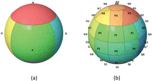
Table 1. Grid characteristics for the first 11 resolutions of the rHEALPix DGGS.

Resolution	Number of Cells	Cell Area (km^2)	√Cell Area (km)
0	6	85010936.954015	9220.138
1	54	9445659.661557	3073.379
2	486	1049517.740173	1024.460
3	4374	116613.082241	341.487
4	39366	12957.009138	113.829
5	354294	1439.667682	37.943
6	3188646	159.963076	12.648
7	28697814	17.773675	4.216
8	258280326	1.974853	1.405
9	2324522934	0.219428	0.468
10	20920706406	0.024381	0.156

Note: All measurements are based on the WGS84 authalic sphere radius of 6371.00718091848 km.

The web service is written entirely in the Python programing language (version 3.6) and makes use of simple HTML forms, Common Gateway Interface (CGI) programing standards, and HTTP protocols to get requests from the client and post results. We chose to use Python because it is simple, easy to read, and is one of the most popular open-source programing languages. Although other languages are more efficient (such as C++), Python better supports our goals of producing a web service that is easy to understand, explore, and improve upon by others.

Although the primary focus of the web service is grid generation, it can also be used to perform coordinate conversion (from geodetic coordinates to cell ID) and bounding cell determination. All three operations are based on the methods and formulas described in Gibb, Raichev, and Speth (2016). In our implementation, grid generation is split into two parts: equatorial and polar. Although the fundamental algorithm is the same for both operations, grid generation in the polar region is mathematically more complex and requires additional input parameters. Therefore, to create a global grid, both the polar and equatorial grid generation operations must be used. The bounding cell operation enables users to determine the cell ID that bounds a region, if it exists. This would be beneficial for users wanting to create a regional grid, say over a country or province (see Section 4.2). The coordinate conversion operation converts geodetic (longitude, latitude) coordinates to cell ID. This is provided to demonstrate how data can be assigned to cells – a requirement in the OGC Abstract Specification.

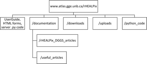
Each operation is accessed through a HTML form which allows users to input a variety of parameters. These parameters are passed to the relevant Python code residing on the server, and results are either sent back to the client or stored in the /downloads folder for users to retrieve. To support sharing of information and reproducible science, all Python code is compressed in a zip folder and can be downloaded from the /python_code folder. Figure 2 shows the web service file structure.

Figure 2. Web service file structure.

Although the rHEALPix DGGS can be defined upon any reference ellipsoid (such as GRS80 or WGS84), this web service works strictly with WGS84 geodetic (longitude, latitude) coordinates. Output files from the grid generation operation are encoded in GeoJSON format (the 2016 GeoJSON Specification (RFC 7946) can be found at http://geojson.org/). We chose GeoJSON because it is a simple, text-based format that supports several geometric objects (such as Point, Linestring, and Polygon). In addition, GeoJSON files can easily be converted to other common file formats such as ESRI Shapefile, using free and open-source GIS software (e.g. QGIS). Using this format, we represent a grid as a ‘FeatureCollection’ where each grid cell is encoded as a ‘Feature’ that comprises its unique identifier and geometry. Figure 3 shows an example GeoJSON output file consisting of nine grid cells.

Figure 3. Example GeoJSON output file consisting of nine grid cells.

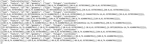
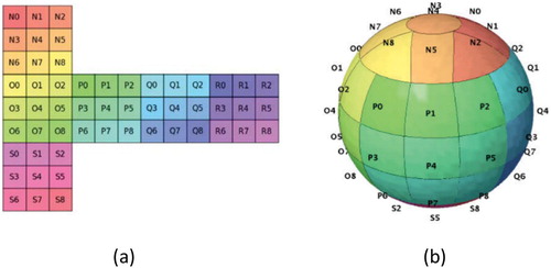
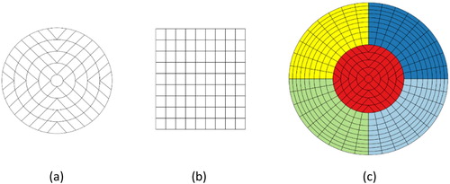
Notice in Figure 3 that the geometry of each cell is defined by four distinct points, which refer to the cell vertices (the initial longitude-latitude coordinate pair is repeated at the end to close the Polygon). The planar representation of the rHEALPix DGGS is a grid of square cells (Figure 4(a)) and square cells can be accurately defined by their vertices. However, when these cells are projected onto the curved surface of the ellipsoid (Figure 4(b)), more points are often needed to preserve boundary shape, particularly at low resolutions. To accommodate this, the web service includes a densification parameter which enables additional points to be introduced into each ellipsoidal cell edge.

Figure 4. (a) The planar grid and (b) ellipsoidal grid of the rHEALPix DGGS at resolution 1 (based on the (0, 0) rHEALPix projection). (Gibb 2016).

To densify ellipsoidal cell edges, we developed a simple algorithm that follows on from the work that determines $\left(x,y\right)$ coordinates of a planar cell’s vertices presented in Section 6 of Gibb, Raichev, and Speth (2016). Our algorithm starts at the upper left vertex and determines the $\left(x,y\right)$ coordinates of all subsequent points in counterclockwise order (to facilitate Polygon creation in GeoJSON format) until the starting point is returned to (Figure 5). To do this, two parameters are required, namely the number of line segments created per planar cell edge after introducing additional points denoted $d$, and the line segment length denoted $w$. At this point, let us denote the $\left(x,y\right)$ coordinates of the upper left vertex as $x_{\mathrm{m}\mathrm{i}\mathrm{n}}$ and $y_{\mathrm{m}\mathrm{a}\mathrm{x}}$ respectively, and the $\left(x,y\right)$ coordinates of the lower right vertex as $x_{\mathrm{m}\mathrm{a}\mathrm{x}}$ and $y_{\mathrm{m}\mathrm{i}\mathrm{n}}$ respectively. We can then determine the $x$ and $y$ coordinates of all points that define the planar cell using$\begin{array}{rl}x\mathrm{c}\mathrm{o}\mathrm{o}\mathrm{r}\mathrm{d}\mathrm{i}\mathrm{n}\mathrm{a}\mathrm{t}\mathrm{e}\mathrm{s}& =\left(\sum _{j=1}^{d+1}\left[x_{\mathrm{m}\mathrm{i}\mathrm{n}}\right]\right)+\left[x_{\mathrm{m}\mathrm{i}\mathrm{n}}+w,x_{\mathrm{m}\mathrm{i}\mathrm{n}}+2w,\dots ,x_{\mathrm{m}\mathrm{i}\mathrm{n}}+\left(d-1\right)w\right]+\left(\sum _{j=1}^{d+1}\left[x_{\mathrm{m}\mathrm{a}\mathrm{x}}\right]\right)\\ & +\left[x_{\mathrm{m}\mathrm{a}\mathrm{x}}-w,x_{\mathrm{m}\mathrm{a}\mathrm{x}}-2w,\dots ,x_{\mathrm{m}\mathrm{a}\mathrm{x}}-\left(d-1\right)w\right]+\left[x_{\mathrm{m}\mathrm{i}\mathrm{n}}\right]\end{array}$and$\begin{array}{rl}y\mathrm{c}\mathrm{o}\mathrm{o}\mathrm{r}\mathrm{d}\mathrm{i}\mathrm{n}\mathrm{a}\mathrm{t}\mathrm{e}\mathrm{s}& =\left[y_{\mathrm{m}\mathrm{a}\mathrm{x}}\right]+\left[y_{\mathrm{m}\mathrm{a}\mathrm{x}}-w,y_{\mathrm{m}\mathrm{a}\mathrm{x}}-2w,\dots ,y_{\mathrm{m}\mathrm{a}\mathrm{x}}-\left(d-1\right)w\right]+\left(\sum _{j=1}^{d+1}\left[y_{\mathrm{m}\mathrm{i}\mathrm{n}}\right]\right)\\ & +\left[y_{\mathrm{m}\mathrm{i}\mathrm{n}}+w,y_{\mathrm{m}\mathrm{i}\mathrm{n}}+2w,\dots ,y_{\mathrm{m}\mathrm{i}\mathrm{n}}+\left(d-1\right)w\right]+\left(\sum _{j=1}^{d+1}\left[y_{\mathrm{m}\mathrm{a}\mathrm{x}}\right]\right).\end{array}$

Figure 5. A schematic of our densification algorithm. The case where one additional point is introduced into each cell edge is demonstrated. Grey circles represent cell vertices, white circles represent additional points, and $w$ is the length of a line segment.

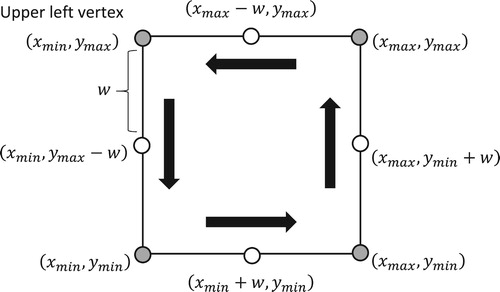
Note, in both cases multiple lists are concatenated (signified by the $+$ operator) to form the final list of coordinates. The final step involves simply projecting all points onto the surface of the ellipsoid, thereby creating an ellipsoidal cell with densified edges.

Finally, with regards to the bounding cell and coordinate conversion operations, it is important to mention that converting geodetic coordinates to cell ID relies on accurately converting a base 10 decimal number in the interval $\left[0,1\right]$ to base 3. Writing a program to perform this computation with reliable results is not simple using floating point representation, yet it is critical for determining the correct cell ID. As a result, our web service makes use of baseconvert (version 1.0.0a4) – a base conversion package from the Python Package Index (PyPI) repository (see https://pypi.org/project/baseconvert).

3.1. Issues and limitations

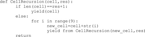
Throughout the development of the web service, we encountered several issues relating to memory usage, file size, and program run time, which we now explain. First, creating high resolution grids means handling extremely large numbers of cells. For example, a grid at resolution 8 has almost 260 million cells (see table 1). That said, the rHEALPix DGGS has a hierarchical and congruent cell structure so it is easy to determine cell ID’s at any resolution using a recursive function. However, if cell ID’s are stored in an array, the computers Random Access Memory (RAM) (typically 8 GB) is quickly used up at high resolutions which prevents the program from running. Therefore, we avoid creating arrays by using a generator function (signified by the yield keyword) as shown in Figure 6. This allows us to step through cell ID’s from the recursive function, working with one cell ID at a time before moving onto the next. Consequently, a RAM limitation is prevented.

Figure 6. Our recursive function to generate cell ID’s at a given resolution. Cell refers to cell ID and res refers to grid resolution.

Second, output file sizes increase dramatically at successive resolutions (by roughly a factor of nine) due to exponential increase in the number of grid cells. Table 2 shows approximate file sizes for various resolution grids generated over a single base cell in the equatorial region (results in the polar region are similar). For example, the output file size for a resolution 2 grid with no cell edge densification (resulting in 81 cells) is approximately 18 KB. At resolution 6 (531441 cells) the output file size is approximately 140 MB. Clearly, at resolution 10 (almost 3.5 billion cells) the output file size would exceed 500 GB. Moreover, if cell edges are densified with additional points, output file sizes are even larger (roughly a 50% increase per additional point). As a result, the condition shown in equation (1(1) $0\le \mathrm{R}\mathrm{e}\mathrm{s}\mathrm{o}\mathrm{l}\mathrm{u}\mathrm{t}\mathrm{i}\mathrm{o}\mathrm{n}-\mathrm{C}\mathrm{e}\mathrm{l}\mathrm{l}\mathrm{I}\mathrm{D}\mathrm{r}\mathrm{e}\mathrm{s}\mathrm{o}\mathrm{l}\mathrm{u}\mathrm{t}\mathrm{i}\mathrm{o}\mathrm{n}<7$(1) ) was placed on the web service to ensure the server could handle client requests.(1) $0\le \mathrm{R}\mathrm{e}\mathrm{s}\mathrm{o}\mathrm{l}\mathrm{u}\mathrm{t}\mathrm{i}\mathrm{o}\mathrm{n}-\mathrm{C}\mathrm{e}\mathrm{l}\mathrm{l}\mathrm{I}\mathrm{D}\mathrm{r}\mathrm{e}\mathrm{s}\mathrm{o}\mathrm{l}\mathrm{u}\mathrm{t}\mathrm{i}\mathrm{o}\mathrm{n}<7$(1)

Table 2. Approximate output file sizes and run times for various resolution grids generated over a single base cell in the equatorial region.

Grid resolution	Number of cells		No Densification		Densification
		File size (KB)	Run time (s)	Points per cell edge	File size (KB)	Run time (s)	Points per cell edge
1	9	2	<1	2	12	<1	10
2	81	18	<1	2	1.0E + 02	<1	10
3	729	1.8E + 02	<1	2	6.7E + 02	<1	7
4	6561	1.6E + 03	1.5	2	6.0E + 03	5	7
5	59049	1.5E + 04	11	2	3.1E + 04	21	4
6	531441	1.4E + 05	83	2	2.8E + 05	187	4

Here, ‘Resolution’ refers to the resolution of the desired grid, and ‘Cell ID resolution’ refers to the resolution of the input cell ID. For example, a grid over cell ID P (resolution 0), at resolution 6 is valid; but a grid at resolution 7 is not. This condition prevents the generation of global grids at resolutions above 6, but it does not restrict regional grids. For example, if a country is contained within cell ID P456 (resolution 3), a regional grid at resolution 9 could be created over the country. This is because the condition restricts the change in resolution, not the resolution itself. In other words, the areal coverage of the input cell ID must decrease to accommodate grid resolutions above 6.

Considering the number of cells in high resolution grids, it should be no surprise that calculating the cell vertices and writing them to an output file takes time. Table 2 shows approximate web service run times for various resolution grids generated over a single base cell in the equatorial region. Evidently, for grid resolutions less than or equal to 6 (with no cell edge densification), the web service responds in adequate time. However, for grid resolution 7 the run time would exceed 10 min, and for grid resolution 8 it would exceed 1 h. This is because run times increase by roughly a factor of eight at successive resolutions which corresponds to the increase in file size. If cell edges are densified with additional points, run times are even longer (roughly a 50% increase per additional point). Therefore, thought must be given to the run time before densifying cell edges with many points, especially as grid resolution increases. Note that in the polar region, projection equations are more complex so run times are approximately three times longer. These performance trends are problematic for high resolution grid requests placed on the web service because they lead to impractically slow response times. Obviously, such long run times are not ideal for a web service because it means maintaining an internet connection to the server for perhaps minutes or hours depending on the grid resolution. Therefore, the resolution condition imposed on our web service also serves to reduce a user’s wait time and server timeout errors.

Our web service is a basic implementation that serves as an easily accessible research tool for anyone wanting to work with equal area quadrilateral grids based on the rHEALPix DGGS. That said, we hope our efforts will promote further research to develop better and more efficient implementations that eliminate the issues we have highlighted. For example, parallel processing seems well suited to the task of creating high resolution grids because the operation could be subdivided and run simultaneously, which would reduce program run time. We acknowledge the fact that placing limitations on our web service and restricting users from creating high resolution global grids is not ideal. However, these limitations can be somewhat avoided by running the code on a computer directly where output file size and program run time may be less of an issue. Therefore, we have provided all of the Python code encompassed within the web service for users to freely download.

4. Discrete grid creation

This section describes how both discrete global grids and regional grids can be created. First, we describe the process to create a global grid. Second, we describe the process to create a regional grid, such as over a country or province, for three distinct cases.

4.1. Global grids

The underlying polyhedron of the rHEALPix DGGS is a cube (hexahedron) which means there are six grid cells at resolution 0, often referred to as base cells. The equatorial region includes base cells O, P, Q, and R ($\sim -{41.9}^{\circ }\le \varphi \le \sim {41.9}^{\circ }$ where $\varphi$ is the geodetic latitude). The polar region includes base cells N (north polar region; $\varphi >\sim {41.9}^{\circ }$) and S (south polar region; $\varphi <\sim -{41.9}^{\circ }$). Figure 1(a) shows the resolution 0 grid of the rHEALPix DGGS (base cells R and S are not visible).

As mentioned earlier, both polar and equatorial grid generation operations must be used to create a discrete global grid. Each operation can create grid cells in their respective base cells and only for one base cell at a time. Therefore, the polar grid generation operation must be used twice and the equatorial grid generation operation four times. To demonstrate, we’ll outline the process to create a resolution 2 discrete global grid.

First, let us create the cells in the north and south polar regions using the polar grid generation HTML form (FormPolarGridGeneration.html). This form has six input parameters: Cell ID, Resolution, Rotation, n, s, and Densification. To create a global grid, the Cell ID must be the base cell (so N or S in this case). Resolution refers to the desired grid resolution, so 2 in this case. The Rotation parameter allows us to rotate the grid by inputting a non-zero decimal degree value (applying a rotation is not needed here but is discussed more for regional grids). Parameters n and s refer to the position of the north and south polar square in the rHEALPix projection, see Gibb, Raichev, and Speth (2016) for more details. Regarding grid creation, parameters n and s only alter the ID assigned to each cell, not the geometry (so we’ll arbitrarily use 0 for both). Lastly, we’ll preserve cell boundary shape on the ellipsoid by introducing additional points into each ellipsoidal cell edge using the Densification parameter. Once the GeoJSON file is generated, it can be downloaded and then visualized in GIS software (using an appropriate polar projection), as shown in Figure 7(a).

Figure 7. Resolution 2 grids over a sample of base cells. (a) Base cell N (North Pole Lambert Azimuthal Equal Area projection, EPSG: 102017). (b) Base cell O (Cylindrical Equal Area projection, ESRI: 54034). (c) Base cells N (red), O (yellow), P (green), Q (light blue), and R (blue) (North Pole Lambert Azimuthal Equal Area projection, EPSG: 102017; colours correspond to Figure 1(a)).

The next step is to create the equatorial region cells using the equatorial grid generation HTML form (FormEquatorialGridGeneration.html). Input parameters are the same except that both n and s parameters are omitted (not relevant to the equatorial region), and there is an additional Output Feature parameter. This parameter enables the user to select cell centroid (point) or cell boundary (polygon) as the output geometry. Once again, the GeoJSON file can be downloaded and then visualized using GIS software (Figure 7(b) shows base cell O).

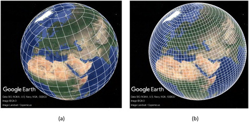
The six GeoJSON files constitute the resolution 2 discrete global grid. These files can be converted to other file formats such as ESRI Shapefile or Keyhole Markup Language (KML), using GIS software. Since a discrete global grid spans the entire globe, it is difficult to clearly visualize all grid cells without distortion or misrepresentation using a map projection. Figure 7(c) shows five-sixths of the globe (base cell S excluded) using the North Pole Lambert Azimuthal Equal Area projection (EPSG: 102017). A more realistic visualization can be achieved using a virtual globe such as Google Earth or ArcGIS Earth. Figure 8(a) shows the resolution 2 discrete global grid in Google Earth after converting the six GeoJSON files to KML format. The whole process was repeated for the resolution 3 discrete global grid, as shown in Google Earth in Figure 8(b).

Figure 8. Discrete global grids at (a) resolution 2 and (b) resolution 3. (© 2018 Google).

4.2. Regional grids

As mentioned earlier, OGC conformant DGGSs provide a solution for handling geospatial big data. In the future, national or regional administrators may find it beneficial to adopt a DGGS framework to reference the large volumes of heterogeneous geospatial data encompassed within their administrative boundaries (Bowater and Stefanakis 2018). To facilitate this, we describe the process to create a regional grid when the region of interest (e.g. province or country) falls in (i) equatorial region, (ii) polar region, or (iii) both the equatorial and polar region.

4.2.1. Equatorial region

The process of creating a regional grid in the equatorial region is straightforward, because all ellipsoidal cells are quadrilaterals bounded by two parallels and two meridians. As a result, cell shape and cell orientation need not be considered (Bowater and Stefanakis 2018). The process consists of the following steps:

1. Determine the base cell (or bounding cell) that contains the region.

2. Generate the GeoJSON file using the web service.

3. Acquire polygon data for the region.

4. Select all cells that intersect the polygon using GIS software.

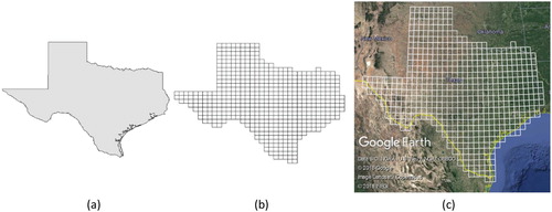
The first step can be accomplished using the bounding cell operation on the web service (FormBoundingCell.html) or by simply comparing the longitudinal extents of the region to those of the base cells. The advantage of using the bounding cell is that it will often be smaller than the base cell, which would increase the highest achievable grid resolution using the web service. Note, if the region spans more than one equatorial base cell, the process must be repeated for each base cell. The second step follows the same process as described for global grids. The third step can be achieved using any open-source data provider such as Natural Earth (https://www.naturalearthdata.com/). For the last step, we opted to convert the GeoJSON file to ESRI Shapefile format using QGIS and work in ArcGIS, because we found the ‘Select by Location’ process in ArcMap to be simple and efficient. Figure 9 shows a resolution 5 quadrilateral grid over the state of Texas, USA.

Figure 9. (a) Source polygon data for the state of Texas, USA from Natural Earth. (b) A resolution 5 quadrilateral grid over Texas (Cylindrical Equal Area projection, ESRI: 54034) and (c) the same grid shown in Google Earth (© 2018 Google).

4.2.2. Polar region

The process of creating a regional grid in the polar region is less straight forward, because cell shape and cell orientation must be considered. The simplest option would be to ignore these features but north–south aligned quadrilateral grids are more familiar to users and link to similar to grids used in remote sensing. It is possible to avoid non-quadrilateral cells and create north–south aligned quadrilateral grids by applying a rotation (Bowater and Stefanakis 2018). Therefore, we will supplement the equatorial process with step 0: Determine the rotation.

To determine the rotation $r$, we need the approximate longitudinal midpoint ${\lambda }_m$ of the region of interest. Then, knowing that north–south aligned cells fall on a line of longitude in $S=\left\{-{135}^{\circ },-{45}^{\circ },{45}^{\circ },{135}^{\circ }\right\}$, we can determine the longitude from $S$ that is closest to ${\lambda }_m$, denoted ${\lambda }_c$, by inspection or simple calculation. Finally, we can calculate $r$ using $r={\lambda }_m-{\lambda }_c$. 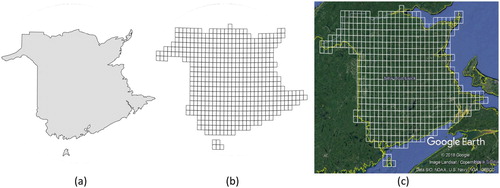We will demonstrate the process by creating a north–south aligned resolution 6 quadrilateral grid over the province of New Brunswick, Canada.

New Brunswick has a minimum geodetic latitude of approximately ${44.5}^{\circ }$ which means it falls in base cell N (north polar region). The approximate longitudinal midpoint ${\lambda }_m$ of New Brunswick is $-{66}^{\circ }$. By inspection, ${\lambda }_c=-{45}^{\circ },$which means $r=-{21}^{\circ }$. To avoid using base cell N in step two, we will determine the bounding cell that contains New Brunswick using the bounding cell operation. Inputting approximate bounding box coordinates and $-{21}^{\circ }$ for Rotation (to ensure the bounding cell is north–south aligned) returns cell N55 as the bounding cell. Using these values for Cell ID and Rotation in step two, enables us to create the desired regional grid, as shown in Figure 10.

Figure 10. (a) Source polygon data for the province of New Brunswick, Canada from Natural Earth. (b) A north-south aligned resolution 6 quadrilateral grid over New Brunswick (North Pole Lambert Azimuthal Equal Area projection, EPSG: 102017) and (c) the same grid shown in Google Earth (© 2018 Google).

4.2.3. Spanning both regions

So far, we have discussed the situations where the region of interest falls in either the equatorial region or the polar region. Here, we outline the process to create a regional grid when the region of interest spans both regions. To demonstrate, we’ll use the country of New Zealand.

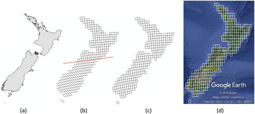
New Zealand spans base cell S (polar region) and base cell R (equatorial region). Although cell shape and cell orientation are not a concern in the equatorial region, ignoring these features in the polar region would lead to a regional grid with an abrupt boundary transition between the two regions, as shown in Figure 11(b). To achieve a north–south aligned quadrilateral grid with a smooth boundary transition, we must apply a rotation. Using the same approach as before for step zero, we get $r={37}^{\circ }$. Step one is made slightly more cumbersome by the fact that we can’t use the bounding cell operation for the whole country, since no bounding cell exists. Therefore, we must determine the two bounding cells (one in each region) separately. Using the rotation determined above, the bounding cell in the equatorial region is R7 and the north–south aligned bounding cell in the polar region is S3. The remaining steps proceed as before, but for each bounding cell separately. Figure 11(c) shows the north–south aligned resolution 5 quadrilateral grid over New Zealand.

Figure 11. (a) Source polygon data for the country of New Zealand from Natural Earth. (b) A non-rotated resolution 5 quadrilateral grid over New Zealand; the red line marks the boundary between the equatorial region and polar region. (c) A north-south aligned resolution 5 quadrilateral grid over New Zealand (South Pole Lambert Azimuthal Equal Area projection, EPSG: 102020) and (d) the same grid shown in Google Earth (© 2018 Google).

As we have shown, applying a rotation is beneficial for creating north–south aligned quadrilateral grids. The process itself simply involves shifting the longitudinal values of a cell’s geometry by the desired amount, which works fine for cells far from the 180th meridian (or anti-meridian). For a cell close to the anti-meridian however, its geometry will include longitudinal values greater than ${180}^{\circ }$ or less than $-{180}^{\circ }$. Geometric objects are not typically defined this way and we have found that GIS software may not recognize or allow such values. Although this is more a problem of interoperability rather than a weakness in the web service, users should be aware that attempting to create a rotated global grid may result in missing cells close to the anti-meridian. Regional grids can be rotated with no issues, as we have shown, but this may not always be the case for regions of interest close to the anti-meridian, or for large rotations.

5. Modeling geospatial entities

The Digital Earth concept is based on a framework that can accommodate all kinds of geospatial information. Therefore, DGGSs must be able to support raster, vector, and point cloud data. In this section, we focus on vector data and present examples that show how GIS software (e.g. QGIS) can be utilized to model points, lines, and polygons at multiple resolutions using quadrilateral grids based on the rHEALPix DGGS. Indeed, GIS software can also handle raster data and point cloud data. Therefore, future work may consider how GIS software can be used to explore how quadrilateral grids based on the rHEALPix DGGS could support raster and point cloud data. In addition, as an alternative to using geoprocessing tools in GIS software, data could be imported into a spatial database such as PostgreSQL/PostGIS where there is access to many inbuilt functions specifically designed for working with spatial data.

One of the key advantages of DGGSs is their ability to model and integrate geospatial data at multiple levels of resolution. This is beneficial because different spatial resolutions or positional uncertainties can be accommodated by matching the resolution level to the properties of the data. In addition, it supports visualization of data sets at different scales which is important for rapid zoom functionality (Goodchild 2018). Purss et al. (2017) briefly discuss the benefits of using a DGGS to integrate multi-resolution data coming from sensor networks and the Internet of Things. Although sensors generally report observations as occurring at point locations, this limits the value of sensor data. Alternatively, the authors suggest using cells of a DGGS to store observations which can record location as well as spatial coverage. In this way, observations from numerous sensors at different resolutions can be integrated, thereby maximizing the value of the data.

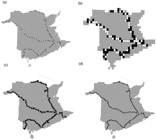
With this in mind, we show how vector data sets can be modeled and integrated at different levels of resolution. The process follows the same steps as described in Section 4.2. First, determine the required rotation to create a north–south aligned grid. Second, determine the base (or bounding) cell that covers the region. Third, create GeoJSON files using the web service. Fourth, acquire the vector data set, be it point, line or polygon data. And finally, use GIS software to determine the cells that intersect the vector features. Figure 12 shows state/territory boundary lines of Australia (excluding Tasmania) modeled at multiple resolutions. Figure 13 shows geographic features in New Brunswick, Canada modeled and integrated at various resolutions; source data obtained from GeoNB (http://www.snb.ca/geonb1/e/index-E.asp) under the GeoNB Open Data Licence.

Figure 12. Australian state/territory boundary lines modeled at multiple resolutions using GIS software. (a) Source data for the country of Australia from Natural Earth. (b) Boundary lines at resolution 4. (c) Boundary lines at resolution 5. (d) Boundary lines at resolution 6. (Cylindrical Equal Area projection, ESRI: 54034).

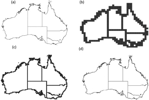
Figure 13. Utilizing GIS software to model geographic features in the province of New Brunswick at various resolutions. (a) Source data for the province of New Brunswick, rail tracks, and rail stations from GeoNB. (b) All features at resolution 6. (c) All features at resolution 7. (d) Province and rail tracks at resolution 8, rail stations at resolution 7. (North Pole Lambert Azimuthal Equal Area projection, EPSG: 102017).

As mentioned earlier, our web service allows users to create quadrilateral grids based on the rHEALPix DGGS where $N_{\mathrm{s}\mathrm{i}\mathrm{d}\mathrm{e}}=3$, which means each cell is divided into a set of 3 × 3 sub-cells at successive resolutions. In other words, the refinement (sometimes called aperture) is one-to-nine. In comparison to other DGGSs, which typically have one-to-three or one-to-four refinements, one-to-nine refinement is uncharacteristically high. Amiri, Bhojani, and Samavati (2013) showed that the minimum refinement for a square is one-to-two, which provides the most gradual transition between cell area at successive resolutions.

Although one-to-nine refinement leads to quick convergence between DGGS and vector representations, as shown in Figures 12 and 13, the large change in cell area at successive resolutions hinders efforts to accommodate different spatial resolutions or positional uncertainties. Therefore, future work should consider the rHEALPix DGGS where $N_{\mathrm{s}\mathrm{i}\mathrm{d}\mathrm{e}}=2$ which has one-to-four refinement. One-to-four refinement does not produce aligned hierarchies like one-to-nine refinement (aligned means the centroid of the parent cell is also the centroid of a child cell), but it has a much smoother transition between cell area at successive resolutions.

6. Conclusion

In this paper, we present our efforts to develop a web service that allows users to create quadrilateral grids based on the rHEALPix DGGS. We have described the implementation of the web service, including notable issues and limitations, and have demonstrated how both discrete global grids and north–south aligned regional grids can be created. In addition, we have shown how these grids can be visualized in map-based and globe-based software. Lastly, we presented examples that show how vector data sets can be modeled and integrated at different levels of resolution using GIS software. Importantly, this work is designed to meet the need of an easily accessible research tool that allows interaction with quadrilateral grids based on the rHEALPix DGGS. To facilitate further research into the implementation and use of such grids, we provide all Python code encompassed within the web service for users to freely download.

With regards to the web service, several directions exist for future work including methods to reduce the resolution limitation so that high resolution global grids can be created; combining the polar and equatorial grid generation operations into a single, more efficient operation; and exploring the use of parallel processing to reduce program run time. It would also be beneficial to explore the rHEALPix DGGS with one-to-four refinement so comparisons against other DGGSs can be made. Aside from the web service, future work should explore how geospatial entities (such as points, lines, and polygons) can be analyzed on the rHEALPix DGGS, including how spatial analysis methods can be applied.

Acknowledgments

We would like to thank the editor and anonymous reviewers for their valuable comments.

Disclosure statement

No potential conflict of interest was reported by the authors.

Additional information

Funding

This work was funded by the Natural Sciences and Engineering Research Council of Canada (NSERC-DG).

References

- Adams, B. 2017. “Wāhi, a Discrete Global Grid Gazetteer Built Using Linked Open Data.” International Journal of Digital Earth 10 (5): 490–503. doi:10.1080/17538947.2016.1229819.
- Amiri, A. M., F. Bhojani, and F. Samavati. 2013. “One-to-two digital earth.” In Lecture Notes in Computer Science (including subseries Lecture Notes in Artificial Intelligence and Lecture Notes in Bioinformatics) (Vol. 8034 LNCS), 681–692. doi:10.1007/978-3-642-41939-3_67.
- Amiri, A. M., F. Samavati, and P. Peterson. 2015. “Categorization and Conversions for Indexing Methods of Discrete Global Grid Systems.” ISPRS International Journal of Geo-Information 4 (1): 320–336. doi:10.3390/ijgi4010320.
- Bowater, D., and E. Stefanakis. 2018. “The rHEALPix Discrete Global Grid System: Considerations for Canada.” Geomatica 72 (1): 27–37. doi:10.1139/geomat-2018-0008.
- Gibb, R. G. 2016. “The rHEALPix Discrete Global Grid System.” IOP Conference Series: Earth and Environmental Science, Vol. 34. doi:10.1088/1755-1315/34/1/012012.
- Gibb, R., A. Raichev, and M. Speth. 2016. The rHEALPix Discrete Global Grid System. doi:10.7931/J2D21VHM. Accessed 17 July 2018. https://datastore.landcareresearch.co.nz/dataset/rhealpix-discrete-global-grid-system.
- Goodchild, M. F. 2000. “Discrete Global Grids for Digital Earth.” Proceedings of the 1st international Conference on discrete global grids, Santa Barbara, CA, USA, 26–28 March 2000.
- Goodchild, M. F. 2018. “Reimagining the History of GIS.” Annals of GIS 24 (1): 1–8. doi:10.1080/19475683.2018.1424737.
- Goodchild, M. F., H. Guo, A. Annoni, L. Bian, K. de Bie, F. Campbell, M. Craglia, et al. 2012. “Next-generation Digital Earth.” Proceedings of the National Academy of Sciences 109: 11088–11094.
- Gorski, K. M., E. Hivon, A. J. Banday, B. D. Wandelt, F. K. Hansen, M. Reinecke, and M. Bartelman. 2005. “HEALPix – a Framework for High Resolution Discretization, and Fast Analysis of Data Distributed on the Sphere.” The Astrophysical Journal 622 (2): 759–771. doi: 10.1086/427976
- Lin, B., L. Zhou, D. Xu, A. X. Zhu, and G. Lu. 2018. “A Discrete Global Grid System for Earth System Modelling.” International Journal of Geographical Information Science 32 (4): 711–737. doi:10.1080/13658816.2017.1391389.
- Ma, T., C. Zhou, Y. Xie, B. Qin, and Y. Ou. 2009. “A Discrete Square Global Grid System Based on the Parallels Plane Projection.” International Journal of Geographical Information Science 23 (10): 1297–1313. doi:10.1080/13658810802344150.
- Mahdavi-Amiri, A., T. Alderson, and F. Samavati. 2015a. “A Survey of Digital Earth.” Computers and Graphics 53: 95–117. doi:10.1016/j.cag.2015.08.005.
- Mahdavi-Amiri, A., E. Harrison, and F. Samavati. 2015b. “Hexagonal Connectivity Maps for Digital Earth.” International Journal of Digital Earth 8 (9): 750–769. doi:10.1080/17538947.2014.927597.
- Mahdavi-Amiri, A., E. Harrison, and F. Samavati. 2016. “Hierarchical Grid Conversion.” Computer-Aided Design 79: 12–26. doi:10.1016/j.cad.2016.04.005.
- Melo, F., and B. Martins. 2015. “Geocoding Textual Documents Through a Hierarchy of Linear Classifiers.” Lecture Notes in Computer Science (Including Subseries Lecture Notes in Artificial Intelligence and Lecture Notes in Bioinformatics) 9273: 590–596. doi:10.1007/978-3-319-23485-4_59.
- OGC. 2017a. “Topic 21: Discrete Global Grid Systems Abstract Specification.” Accessed 2 August 2018. http://docs.opengeospatial.org/as/15-104r5/15-104r5.html.
- OGC. 2017b. OGC announces a new standard that improves the way information is referenced to the earth. Accessed 2 August 2018. http://www.opengeospatial.org/pressroom/pressreleases/2656.
- Purss, M. B. J., S. Liang, R. Gibb, F. Samavati, P. Peterson, J. Ben, C. Dow, and S. Saeedi. 2017. “Applying Discrete Global Grid Systems to Sensor Networks and the Internet of Things.” IEEE international geoscience and remote sensing Symposium (IGARSS), Fort Worth, TX, 2017, 5581–5583. doi:10.1109/IGARSS.2017.8128269.
- Roşca, D., and G. Plonka. 2011. “Uniform Spherical Grids via Equal Area Projection From the Cube to the Sphere.” Journal of Computational and Applied Mathematics 236 (6): 1033–1041. doi:10.1016/j.cam.2011.07.009.
- Sahr, K. 2015. DGGRID version 6.2b: User Documentation for Discrete Global Grid Generation Software. Accessed 7 July 2018. http://webpages.sou.edu/~sahrk/dgg/dggrid.v62/dggridManualV62.pdf.
- Sahr, K., D. White, and A. J. Kimerling. 2003. “Geodesic Discrete Global Grid Systems.” Cartography and Geographic Information Science 30 (2): 121–134. doi:10.1559/152304003100011090.
- Sherlock, M. 2017. “Visualisations on a Web-Based View-Aware Digital Earth.” Master’s Thesis, University of Calgary.
- Sirdeshmukh, N. 2018. “Utilizing a Discrete Global Grid System For Handling Point Clouds With Varying Locations, Times, and Levels of Detail.” Master’s Thesis, Delft University of Technology.
- Vince, A., and X. Zheng. 2009. “Arithmetic and Fourier Transform for the PYXIS Multi-Resolution Digital Earth Model.” International Journal of Digital Earth 2 (1): 59–79. doi:10.1080/17538940802657694.