Producing consistent visually interpreted land cover reference data: learning from feedback

ABSTRACT

Reference data for large-scale land cover map are commonly acquired by visual interpretation of remotely sensed data. To assure consistency, multiple images are used, interpreters are trained, sites are interpreted by several individuals, or the procedure includes a review. But little is known about important factors influencing the quality of visually interpreted data. We assessed the effect of multiple variables on land cover class agreement between interpreters and reviewers. Our analyses concerned data collected for validation of a global land cover map within the Copernicus Global Land Service project. Four cycles of visual interpretation were conducted, each was followed by review and feedback. Each interpreted site element was labelled according to dominant land cover type. We assessed relationships between the number of interpretation updates following feedback and the variables grouped in personal, training, and environmental categories. Variable importance was assessed using random forest regression. Personal variable interpreter identifier and training variable timestamp were found the strongest predictors of update counts, while the environmental variables complexity and image availability had least impact. Feedback loops reduced updating and hence improved consistency of the interpretations. Implementing feedback loops into the visually interpreted data collection increases the consistency of acquired land cover reference data.

KEYWORDS:

• Land cover mapping
• learning curve
• validation
• visual interpretation

1. Introduction

Global land cover and land use maps are important for various planning and management activities (Lillesand, Kiefer, and Chipman 2008; Zhao et al. 2014). For map validation and calibration, a reference dataset of greater quality than the map itself is needed. Genuine ground truth would supply such high-quality data, but populating a global dataset with a sufficiently large sample of field measurements is extremely costly. Visual interpretation of high-resolution imagery is a feasible alternative acquisition method.

The reference data collected by means of visual interpretations of remotely sensed data, even when delivered by well-trained professionals, are subject to interpreters’ variation. Due to their perception of different land cover types, interpreters may largely disagree on category labels they assign to sampling units based on visual interpretation of imagery. For example, in an experiment set up by Powell et al. (2004), a group of five trained interpreters produced reference data by visual interpretation of aerial videography. The assigned land cover type differed for almost 30% of the sample units. Tarko, de Bruin, and Bregt (2018) compared shadow areas interpreted by 12 individual interpreters and found that the intersection of the shadows digitised by the interpreters was less than 3% of their union. Such disagreement among interpreters is indicative of labelling error, which may have a substantial impact on the later uses of the reference dataset. McRoberts et al. (2018) showed that interpretation error induces bias into the stratified estimator of forest proportion and recommend to use input from at least three experienced interpreters to mitigate this effect. Sample data interpreted by multiple interpreters boosts the accuracy of visually interpreted datasets (McRoberts et al. 2018). In addition to collecting reference data by trained individuals, vast number of land cover interpretations can be obtained from volunteered geographic information (VGI). To overcome the issue of unknown quality of such data, the use of control locations with known land cover were used (Comber et al. 2013). However, there are no concrete methods for implementing VGI data or utilise information about the quality of individual contributors (See et al. 2015).

Another way forward for increasing the consistency of visually interpreted data is to include a review in the data acquisition process. This approach was used by Zhao et al. (2014), who created a validation dataset for a global land cover map. Samples were collected with the help of experts, later checked by those experts from the group with ‘outstanding skills in image interpretation’ and finally checked, and if necessary adjusted, by the most experienced interpreter. To achieve satisfactory accuracy of dataset, as much effort as two rounds of review were implemented, but no feedback was provided to the experts during the data collection.

In the domain of education, learning, and instruction, feedback is considered to be a fundamental principle for efficient learning. It is defined as post-response information provided to learners to inform them of their performance (Narciss 2008). Feedback loops are considered efficient in various research fields, and it is a basic concept in the education science where a feedback loop is needed to adjust the actions of teachers to ensure that a student learns (Boud and Molloy 2013). Feedback loops are also efficient in the field of automated interpretation of images. An example of active machine learning algorithms benefitting from interpreter feedback is presented in Tuia and Munoz-Mari (2012). In the domain of medical image interpretation, where the misinterpretation of clinical exams is a delicate issue, a good training process is of high importance. da Silva et al. (2019) proposed a training platform where the application compared the image analysis performed by a student with the teacher’s and provided feedback to the user. The measures of teaching efficiency were left for the future work, but the platform usability assessment done by the students was positive.

Similar to the examples above, collecting global land cover reference data by visual interpretation can be expected to benefit from feedback loops. To assess the effectiveness of feedback provided, individual learning curves can be characterised. Learning curves are mathematical models to model skill acquisition, representing the relationship between practice and the associated changes in behaviour (Speelman and Kirsner 2005; Lallé, Conati, and Carenini 2016).

Our analyses concern acquisition of a validation dataset for the Copernicus Global Land Service (CGLS) Dynamic Land Cover project. The CGLS Dynamic Land Cover project provides a global land cover mapping service as a component of the Land Monitoring Core Service of Copernicus, the European flagship programme on Earth Observation (CGLS 2019). The acquisition of the validation dataset for this project bears similarity with the work of Zhao et al. (2014), in which visual interpretations of reference land cover were reviewed. In addition, feedback loops concerning individual interpretations were provided. Validation is performed according to the protocols of the Committee on Earth Observation Satellites – Land Product Validation Subgroup (CEOS-LPV protocols, CEOS 2019), and the data follow the design of a multi-purpose validation dataset, aiming to be applicable for multiple map assessments (Tsendbazar et al. 2018).

Given that land cover visual interpretations may differ between interpreters, more consistent land cover reference data can be achieved when there is more agreement between the multiple interpreters on land cover visual interpretations. In this paper, we assess whether feedback loops can improve the consistency of validation data for global land cover maps. We also assess the explanatory power of variables related to image interpretation such as interpreter identifier, feedback stage, or location of the sample, in predicting the agreement level between the interpreters and the reviewers regarding visual interpretations of land cover.

2. Methods

2.1. Experimental setting

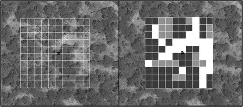
To collect a global land cover reference dataset, sample sites were selected using a global stratification by Olofsson et al. (2012), which is based on Köppen bioclimatic zones (Peel, Finlayson, and McMahon 2007) and human population density. Tsendbazar et al. (2018) provide details on the used sampling design. The validation sample consisted of 15,743 sites of approximately 1 ha. The sites were divided between regional interpreters chosen in a similar way as described by Tsendbazar et al. (2018, 2019). Interpreters then interpreted and mapped sites appointed to them. The sample site is composed of 100 equally sized square elements. Interpreters assigned a dominant land cover class to each of these elements (Figure 1). The sample size handled by individual interpreters ranged between 130 and 1194, with an average of 685 sites. Sample sites were offered in random order, so that the individual interpreted different land cover types over the course of the validation task.

Figure 1. Example of a sample site. Left – the sample site (approximate size 1 ha) comprising of 100 equally sized square elements (approximate size of an element 10 m by 10 m). Right – interpreted sample site with three different land cover classes assigned to every block (white, grey, and black indicate different dominating land cover classes at element level). Source: Tsendbazar et al. (2018).

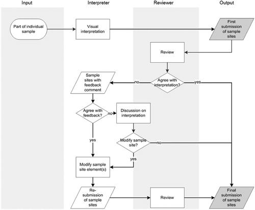
During the data collection process, four review cycles were conducted by two global land cover reviewers (contracted within context of the (CGLS) Dynamic Land Cover project) who provided feedback on each interpretation to the regional interpreters. In case of disagreement on the interpretation, the regional interpreters either rebutted the feedback or modified their interpretations where necessary. After finishing a feedback loop and potential modifications by the regional interpreters, the interpreters proceeded to interpret and label the next batch. For the majority of interpreters, the feedback loops were designed to first provide a quick feedback on a batch of 10–20 sample sites within few days after submission by the interpreters. Next, approximately 50 sample sites were reviewed followed by a batch of some 100 sample sites, and finally, the remaining sample sites were reviewed and feedback was passed to the regional interpreters. Data collection and the review process are schematised in Figure 2.

Figure 2. Flowchart presenting the simplified process of sample collection, review, and feedback in one of the four loops; flowchart shapes with grey background indicate compared data.

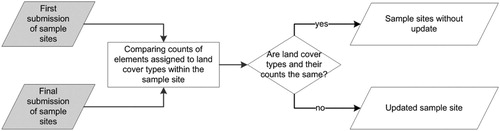
If the regional interpreters (or, in exceptional cases, a reviewer) modified land cover type for at least one of the 100 elements of a sample site, the entire sample site was considered to be re-submitted. By comparing counts of elements assigned to land cover types at the first submission and the final submission of given sample site, updated sample sites were identified (Figure 3). In what follows, such a sample site is referred to as an ‘updated sample site’. Note that not every sample site with modification of element results in an updated sample site, for example, re-submitted sample site, where the land cover assigned to elements has been modified, but the counts of elements assigned to land cover type are the same.

Figure 3. Flowchart for identifying sample sites that are updated based on element counts.

In a post-processing step, the proportions of land cover types at 1 ha site level were translated into the simplified CGLS legend categories (see the legend categories in Table 1 and class definitions in CGLS (2019) and Tsendbazar et al. (2018)). In the reference data, both wetland and burnt area were treated as conditions of land cover rather than as separate classes. For reasons of simplicity, these conditions were omitted in the current data acquisition exercise. Sample sites with a CGLS legend update were identified by comparing the CGLS legend categories assigned at the first and the final submission (Figure 4). Note that not every updated sample site results in a change in CGLS legend category.

Figure 4. Flowchart for identifying sample sites that are updated based on the CGLS legend category.

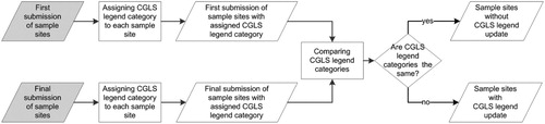
Table 1. Selected factors potentially influencing the MPU.

Category	Factor	Description	Values
Personal	Interpreter identifier	Individual identification of the interpreter	23 Interpreters, id labels from 1 to 23 (nominal scale)
	Experience	Ordinal categorisation of years of experience in land cover/land use visual interpretation of the interpreters	Five ordinal categories: up to 2 years; 2–3; 4–5; 6–9; 10 and more
	Interpretation duration	Time used to submit the sample site by the interpreter	From 0 to 30 min (continuous scale)
Training	Feedback stage	Ordinal categorisation of the review cycle at which the sample site was mapped	Four ordinal categories: from first to fourth stage (review cycle)
	Timestamp	Time (seconds) between the first collected sample site (time 0) and the submission of any other sample site. Registered for each interpreter, for first submission of given sample site	From 0 to 10,262,630 s (16 weeks 6 days 18 h 43 min 50 s) (continuous scale)
Environmental	Complexity	Number of different land cover types identified and mapped within the sample site final submission	Integers from 1 to 6
	Image availability	Four-level ordinal categorisation explained above (Section 2.2)	Four ordinal categories: no information on season, non-growing season only, growing season only, information on both seasons
	Land cover	Final land cover assigned to the sample site according to the CGLS legend category	Nine categorical labels: bare, closed forest, crop, grass, open forest, shrub, snow and ice, urban, water (nominal scale)
	Location	Longitude and latitude of the sample site (treated separately)	84°N–56°S, 180°W–180°E (continuous scales)

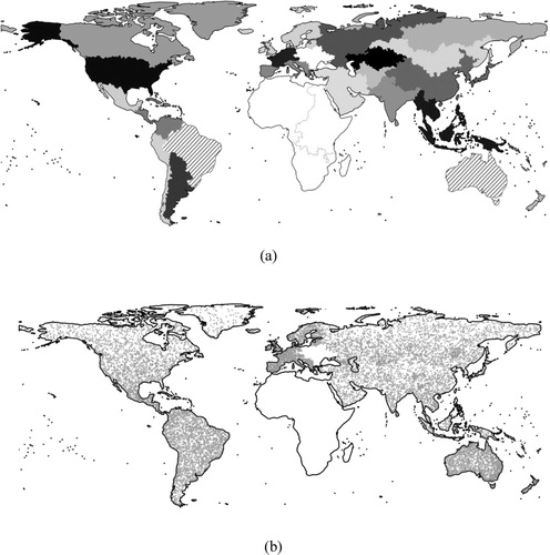
Data acquisition involved 27 regional interpreters distributed over 25 regions. Following the finding that volunteers interpreting land cover perform better in case of samples near their familiar places or samples with their familiar climate type (Zhao et al. 2017), experienced interpreters involved in our experiment were selected based on their region of expertise. In two regions, data collection was done by two interpreters to handle the large sample size; the other regions had one interpreter each (Figure 5(a)). All interpreters were experienced in satellite-based land cover analysis and image interpretation. All of them were provided with a mapping tutorial explaining the interface for data collection, the land cover interpretation specific for the project, and the interpretation keys. Since the learning curves of the interpreters most likely changed already after getting acquainting with the tutorial, the starting point of our analysis coincides with the moment the tutorial was finished. Collection of the first few points was organised as an on-line training exercise that was tailored to each interpreter’s needs. Three interpreters mapping three regions in Africa had prior knowledge and experience with the project because they had contributed to a similar task before (Tsendbazar et al. 2018). The results produced by those interpreters were excluded from the experiment, as their learning curves were expected to be different from the interpreters who took the activity for the first time (Figure 5). For similar reasons, data of one interpreter mapping, Eastern Europe was excluded from the analysis (Figure 5). In total, the input of 23 interpreters was analysed for the purpose of this paper. Figure 5 shows the spatial distribution of sample sites.

Figure 5. (a) Validation regions. Grey tones indicate regions interpreted by single interpreters; hatch patterns indicate regions interpreted by two interpreters; white fills indicate regions outside the scope of this paper’s experiment. (b) Distribution of sample sites (grey dots) in the scope of this paper experiment.

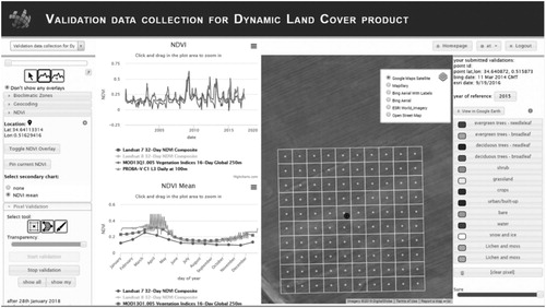
The CGLS land cover validation data were collected using a dedicated branch on the Geo-Wiki Engagement Platform (http://www.geo-wiki.org). Figure 6 shows a screenshot of the validation data collection interface. Through the interface, several remote sensing images were interpreted, and the prevalent land cover was assigned to each element. Land cover types to be assigned are listed in the rightmost panel of Figure 6. Interpreters could use several data layers, i.e.:

• openly-available very-high-resolution Google and/or Bing imagery;

• Natural Colour Composite and False Colour Composite Sentinel-2 imagery from 2015;

• time-series imagery from Sentinel 2;

• normalised difference vegetation index (NDVI) time-series from Landsat 7 32-Day, MOD13Q1.005 16-Day Global 250 m, PROBA-V C1 Daily at 100 m; and/or

• map with Köppen-Geiger bioclimatic zones (Olofsson et al. 2012).

Interpreters were also offered functionality to export the sample site to Google Earth, which allowed viewing historical imagery. Whenever possible, Google image was the main data layer to be used. Interpretation targeted to represent land cover in the growing season of 2015. This implies that seasonal changes in land cover were not considered in this research.

Figure 6. Screen shot of Geo-Wiki portal interface for land cover validation. The leftmost panel allows selection of additional data such as NDVI profile or bioclimatic zone; the second panel from the left shows the local NDVI; the third panel from the left displays the sample site with chosen background image; the rightmost panel shows the list of land cover types.

2.2. Exploratory analyses

We expected that regional interpreters interpreting the validation samples gained practice over time and that the feedback loops induced the learning effect. We quantified the learning effect with the update level changing in time for each individual. Updates upon feedback were counted and expressed as a percentage relative to the total number of sample sites submitted by the interpreter concerned up to a given moment in time. From here on these percentages are referred to as ‘momentary percentage of updates’ (MPU).

We researched nine factors as potential explanatory variables, clustered in three categories (training, personal, and environmental) and listed in Table 1. Note that interpretation duration was calculated under the assumption that a submission gap longer than 30 min corresponded to a break taken by the interpreter. Interpretation duration could not be computed for the first submission after any break. As a consequence, 1152 out of the 15,743 sample sites lacked data of interpretation duration.

To assess the relationship between interpreter identifier and MPU, we investigated individual learning curves of the interpreters as well as a collective learning curve (aggregated over all interpreters). Learning curve is expressed as a graph indicating normalised timestamp in the x-axis and MPU in the y-axis.

To approximate interpreter’s proficiency in land cover interpretation, we asked the interpreters about their years of experience with land cover, land use, and vegetation cover mapping in the form of a survey. Possible responses were grouped in five ordinal categories:

• up to 2 years;

• from 2 up to 4 years;

• from 4 up to 6 years;

• from 6 up to 10 years;

• 10 and more years of experience.

Image availability was assessed using data from the work of Lesiv et al. (2018), which presents the availability of Google Earth imagery (with resolution <5 m) across the world’s land surface for different growing seasons. Bing images were not included in their seasonal analysis. The world is represented by a 1° grid holding information concerning seasons on available imagery in four ordinal categories:

• no information on seasons;

• images taken only in non-growing season;

• images only in growing season;

• images from growing and non-growing seasons.

Through overlay, we determined the availability of Google images in growing seasons for each sample site.

The influence of each factor on the MPU was assessed using scatter plots, bar graphs, box plots (McGill, Tukey, and Larsen 1978), and Spearman’s rank-order correlation. Factors can be correlated because some of them represent similar attributes, such as timestamp and feedback stage. As a diagnostic for RF analysis, we used a correlation matrix. For obvious reasons, categorical factors (land cover class and interpreter identifier) were excluded from the correlation analysis.

All plots were created using R software for statistical computing (R Core Team 2017) using the ‘graphics’ packages for box plots (R Core Team 2017), the ‘plotly’ package for scatter and bar plots (Sievert 2018), and the ‘corrplot’ package for correlation matrix (Wei and Simko 2017).

2.3. Modelling the learning effect

RF regression analysis was chosen to identify the importance of factors for describing the learning effect. The input factors in Table 1 were used as explanatory variables. Random forest regression analysis was chosen because tree-based models can handle correlated input data, non-linear relationships, and mixtures of categorical and numerical data types. Moreover a RF model is non-parametric, accounts for interactions, and is robust against over fitting (Breiman 2001, 2002).

Since RF cannot handle missing predictor values, we analysed two models:

• a model using all (ten) explanatory variables but excluding sample sites without data on interpretation duration (14,591 sites were used);

• a model using all sites (15,743 sites) but without the interpretation duration factor (nine explanatory variables were used).

First model allows importance identification of all factors while the second model uses all available input sites. The two models are complementary.

The parameter settings in the RF regression analysis were as follows: 500 trees, three variables tried on each split and a minimum of five observations in the terminal nodes. Factors were treated as numeric variables, except for land cover class and interpreter identifier, which were treated as categorical variables in the RF regression analysis. From the model we obtained:

• mean square difference (MSD, sum of squared residuals divided by the number of sample sites in the dataset);

• percentage of variance explained for the entire validation dataset (formula: 1 – MSD/variance of the dataset);

• variable importance (reported as % increase of MSD). Variable importance was estimated with out-of-bag cross-validation as a result of variable being permuted.

To assess the stability of the RF results, we ran the models 15 times and reported average values of MSD, percentage of variance explained for the entire validation dataset, and variable importance, as well as the range (smallest and largest value) obtained from the 15 iterations for each value. Goodness of fit is indicated by the percentage of variance explained and MSD, while variable importance was assessed by the percentage increase of MSD.

The RF regression analysis was performed using R software (R Core Team 2017) using the ‘randomForest’ package (Liaw and Wiener 2002).

3. Results

3.1. Exploratory analysis

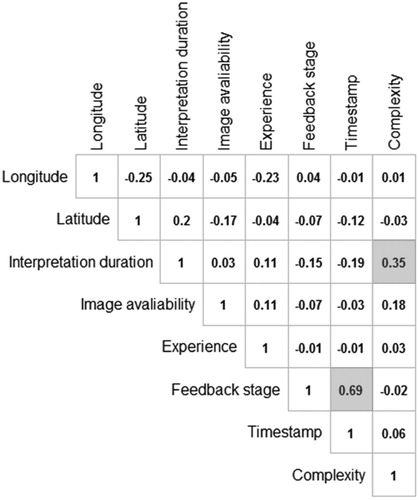
Figure 7 shows the correlation matrix of selected factors that were deemed to influence the MPU. As expected, timestamp and feedback stage are strongly correlated, which can be explained by the second factor being a discrete representation of the first one. Note also the observed positive correlation between interpretation duration and complexity owing to visual interpretation of complex scenes being usually more time consuming. Location factors (longitude and latitude) showing negative correlation with interpreter’s experience are considered as random effect of the choice of regional interpreters.

Figure 7. Correlation matrix of factors potentially influencing the momentary percentage of update. The two highest correlation values are marked by a grey background.

3.1.1. Personal factors

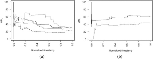
Figure 8 shows selected learning curves for individual interpreters with normalised timestamp factor on the x-axes. MPU varied in time and per interpreter and changed from 0 up to 100 for different interpreters at different moments during the mapping process. For Figure 8(a), the curves indicate a general downward trend in time; those correspond to interpreters who learned from the feedback loop. These curves represent positive learning effects. Positive learning effects were observed for the majority of interpreters who were characterised by high MPU at the beginning of the task and lower MPU towards the end of the data collection process. In Figure 8(b), the curves show upward MPU trends, representing interpreters to whom the feedback did not bring the expected learning effect. Learning curves strongly differed between individual interpreters (Figure 8). Moreover, learning effects also changed over time for individual interpreters (see Figure 8). When calculating the percentage of updated sample sites per feedback loop for each interpreter, only three of them reached the highest update percentage in the third or fourth loop, meaning that the positive learning effect is not confirmed for those three individuals.

Figure 8. (a) Exemplary learning curves of interpreters (indicated by different grey shades) with positive learning effect. (b) Exemplary learning curves of interpreters without positive learning effect (indicated by different grey shades).

Figure 9 shows the aggregated learning curve over all regional interpreters. The solid black line with the downward trend means that there was a positive learning effect over the entire group of interpreters on average because the MPU dropped in time and finally reached 30% of updated sample sites. Translated into the CGLS legend category at the sample site level, the final update percentage on CGLS legend category is 9% (solid grey line in Figure 9).

Figure 9. Learning curves aggregated over all regional interpreters.

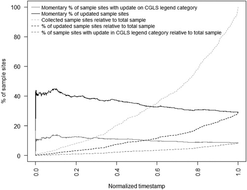
The dashed lines in Figure 9 show the update percentage relative to the total sample. The lightest grey line shows that the data collection increases in time, and the exponential-like shape of the plot indicates that data collection was more intensive during the last stretches of the project. The darkest line indicating the percentage of updated sample sites shows a stable increase over time, with slightly steeper slope of the plot from the 0.8 of normalised timestamp of the collection task. Similarly, for the percentage of sample sites with CGLS legend update, the percentage increase plot seems linear (medium-grey colour).

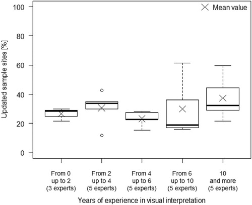
Figure 10 shows the distribution of percentage of updated sample sites per experience category. The update percentage is expressed relative to an interpreter’s individual sample size, and the category is represented as years of experience in land cover/land use visual interpretation. Regional interpreters participating in the land cover reference data collection were evenly distributed concerning years of experience (three interpreters with the least experience category and five interpreters in each of the other categories). The lowest mean value of the update percentage for the individual interpreters was for the group with four to six years’ expertise, and the highest mean value concerned interpreters with the longest experience. Less experienced interpreters (less than six years of experience) tended to have similar update rates, while interpreters with more than six years of experience varied considerably in terms of update rates. The percentage of updated sample sites substantially varied between individual regional interpreters: the lowest update percentage was 12%, the highest 62%, and the mean 30% (Figure 10).

Figure 10. Distribution of updated sample sites per interpreters’ experience category.

3.1.2. Training factors

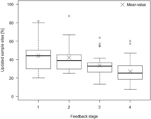
The box plot in Figure 11 shows percentage of updated sample sites grouped by feedback stage. The mean and the median of update percentage decreased over subsequent feedback stages. The spread of update percentages for individual feedback stages is caused by the large variation among the interpreters.

Figure 11. Distribution of updated sample sites per feedback stage.

3.1.3. Environmental factors

The exploratory analysis of relationships between environmental factors and interpretation updates are shown in Figure 12. Figure 12(a) concerns land cover complexity expressed by the number of land cover types within a sample site. The majority of the sample sites (∼89%) did not have more than three different land cover classes. The update percentage increased with the increasing number of land cover classes up to five (Figure 12(a)). Note that fewer than 4% of all sample sites had five or more different land cover classes, and therefore, the categories with the highest number of land cover may not be representative for drawing conclusions on update percentage.

Figure 12. Environmental category analysis: (a) updated sample sites per given complexity (black dots) and percentage of sample sites with given complexity relative to total sample (grey bars); (b) updated sample sites per final land cover class (black dots) and percentage of sample sites with given CGLS legend category relative to total sample (grey bars); (c) distribution of updated sample sites per image type available for mapping; (d) distribution of updated sample sites per CGLS legend category.

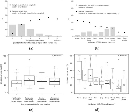
Figure 12(b,d) shows the total sample categorised by the final CGLS legend. Figure 12(b) illustrates that the majority of sample sites (63%) had forest (closed and open) or grass as a final CGLS legend category. The urban land cover had only 3% of sample sites from the total sample, but the update percentage was the highest from all CGLS legend categories (44%). The lowest update percentages were for the classes ‘water’ and ‘snow and ice’ (12% and 11%, respectively).

Figure 12(c) shows the total sample categorised by the image type available for mapping and the distribution of percentage of updated sample sites with the same image availability, calculated for each interpreter. For more than half (59%) of the total sample, images with at least growing season were available. The percentage of updated sample sites relative to all sample sites with given image availability varied between the interpreters: most for the updated sample sites with images available only in the non-growing season (from 10% to 90%) and least for the updated sample sites with images available only in the growing season (from 11% to 54%).

Figure 12(d) shows the distribution of the percentage of updated sample sites for individual interpreters against the final CGLS legend category. Closed forest, open forest, and grass cover had the largest dispersion of the update percentage among the interpreters as well as the highest mean update percentage values.

3.2. Random forest

In Table 2, we report the percentage of variance explained and MSD results of the RF regression model. Table 2 shows that the fit is high for both versions of the model. The mean from 15 runs explained 98.0% and 96.5% of variance of the MPU for the individual interpreters in first and second model, respectively, and the range was less than 1% in both cases. The MSD value was higher for the second version on the model (5.5%) and almost double compared with the first model version.

Table 2. Goodness of fit statistics of the RF regression model based on 15 iterations.

Value	Model version
	(1) Dataset subset	(2) Full dataset
	Mean (range)	Mean (range)
Variance explained, %	98.0 (97.9–98.0)	96.5 (96.4–96.6)
MSD, %	3.2 (3.1–3.2)	5.5 (5.5–5.7)

For both model versions, the order of mean importance value was the same for the first three factors: interpreter identifier, timestamp, and feedback stage from the personal and training categories. From those, the first two factors were ranked the same in all single model runs. In Table 3, we reported the mean importance of the input factors and in parentheses their range in 15 runs. The most important variable for both models and in all runs was the interpreter identifier, with 76.2% mean importance in first model and 80.0% mean importance in second model. The second-most important factor was the timestamp and the third-most important factor was the feedback stage. In the first model, the range of the feedback stage importance was overlapping with the next in order – experience factor range; therefore, in two single runs, the order of feedback stage and experience factors was swapped. The two least-important factors were complexity and image availability, with swapped order between the model versions and between the runs within the model. Their mean importance was between 11.6% and 13.2%, with the ranges from 9.1% to 15.1%.

Table 3. Importance of the RF explanatory variables based on 15 iterations.

Factor	Model version
	(1) Dataset subset	(2) Full dataset
	Mean importance, % (range)	Mean importance, % (range)
Interpreter identifier	76.2 (73.1–80.4)	80.0 (77.3–84.6)
Timestamp	65.8 (61.9–68.9)	69.6 (66.9–72.1)
Feedback stage	34.3 (30.5–37.4)	35.9 (33.1–38.6)
Experience	32.1 (30.9–33.8)	31.3 (29.3–33.1)
Location (latitude)	30.8 (29.7–32.3)	31.4 (30.0–32.4)
Location (longitude)	26.6 (24.9–29.3)	27.5 (25.7–29.9)
Land cover	22.6 (21.1–24.9)	19.1 (17.5–21.5)
Interpretation duration	19.0 (16.0–21.8)	–
Complexity	13.2 (11.4–14.1)	11.6 (9.6–12.6)
Image availability	12.6 (10.9–15.1)	12.0 (9.1–14.0)

To assess the importance of feedback, we run once RF regression with parameter settings as above, but without timestamp variable. The model fit was high, at 92.2%, with MSD of 12.1%. Regarding the importance of explanatory variables, by far the most important factor was feedback stage (228.2%), followed by interpreter identifier (78.9%), land cover (32.1%), and latitude, (30.1%). The least important was image availability (14.1%).

4. Discussion

4.1. Interpreter identifier and training factors

We assessed basic factors influencing learning effect represented by MPU. The most important factors were interpreter identifier, timestamp, and feedback stage (Table 3). Timestamp and feedback stage were strongly correlated (Figure 7), as the latter can be considered a discrete representation of the first one. In the RF regression model, timestamp has a finer granularity than feedback stage, which may explain its higher importance rating compared with the four-level feedback stage (Table 3). Despite its coarser granularity, feedback stage immediately follows timestamp in the importance ranking (Table 3). This implies that it adds information to the timestamp variable. Assessing the model without the timestamp factor, feedback stage comes in first place as the most important explanatory variable influencing the MPU. Feedback adds to the fact that, with time, interpreters gained more knowledge on the project and confidence using the software through autonomous learning or ‘learning by doing’ (Schank, Berman, and Macpherson 1999).

Interpreter identifier and timestamp, together with the MPU, are presented as individual learning curves, and in our study a decrease of MPU for individuals indicated a positive learning effect of the regional interpreters (Figure 8(a)). The biggest drops in the MPU for various interpreters were in different moments of the normalised time (Figure 8(a)). All curves were distinct, emphasising the interpersonal differences between the interpreters. Despite regular review and feedback loops, the positive learning effect is not confirmed for three interpreters out of 23 (Figure 8(b)). The reasons of this finding are not clear to the authors.

The interpreter identifier is a categorical factor, with 23 distinct values. Since in the RF method the variable importance measures for categorical predictor variables are affected by the number of categories (Strobl et al. 2007), we repeated variables assessment with the ‘cforest’ function from the ‘party’ package (Hothorn et al. 2006; Strobl et al. 2008, 2007). This function provides unbiased variable selection in the individual classification trees (Strobl et al. 2007). The importance of the order of factors was identical to the order reported in Table 3, confirming our earlier results. Despite the many levels of the interpreter identifier, its importance was prevalent, meaning that this remains the most important factor influencing the positive learning effect of the interpreters.

The group of interpreters collected less intensively at the beginning of the task and collected many more sample sites towards the end of the mapping task: Figure 9 shows that only 30% of the sample sites were collected half way during the assignment. This might be also partially a result of more frequent feedback loops at the beginning of data collection. However, the last feedback loop had the lowest update percentage (Figure 11). A regular review without feedback is one of the ways to increase the consistency of collected dataset (Zhao et al. 2014). In the work of Zhao et al. (2014), sample sites collected by interpreters were checked by one reviewer and adjusted when necessary. Such a procedure can be prone to the subjectivity of the reviewer’s final assignment of land cover. In our data collection design, feedback on all sample sites was implemented and provided to the regional interpreters. In case of disagreement, interpreters had a possibility to rebut the reviewer’s feedback, and therefore, to reduce the reviewer’s subjectivity of land cover interpretation. The mean and the median of update percentage for individual interpreters was decreasing in the subsequent feedback stages (Figure 11), meaning that the interpreters and the reviewers agreed more often on the sample site interpretation at the later stages of the data collection process.

In the experiment of Powell et al. (2004), five trained interpreters produced reference data by visual interpretation of aerial videography, where the assigned land cover type differed for almost 30% of the sample units. In our study, the MPU at the end of our experiment showed that 9% of sample sites were updated regarding CGLS legend category (Figure 9). This update percentage highlights that fewer updates were required thanks to the feedback stages implemented in this study.

4.2. Personal factors

Personal factors influenced the learning effect of the individuals. This result is similar to a study done by Van Coillie et al. (2014) where a web-based digitisation exercise performance was mainly determined by interpersonal differences.

The number of years of experience in visual interpretation was previously used as a measure of interpreter expertise (Mincer 1974). Our results (Table 3) suggest that the interpreter identifier is twice as important as the number of years of experience. This finding indicates that there are large differences between interpreters, which are not captured by years of experience.

In visual interpretation projects with many actors, it is challenging to engage a uniform group of interpreters with similar interpretation skills, regional expertise, and experience. In our research, interpreters had different years of experience and their percentage of updated sample sites varied, even for individuals within the same interpreter’s experience category (Figure 10). In our experiment, all interpreters had remote sensing background, previous experience in land cover classification and knowledge on the region of their expertise. In the absence of detailed information about the experience of interpreters, we chose the number of years of experience in land interpretation as a feasible indicator of individual experience. The number of years of experience may be considered an insufficient or merely partial indicator of interpretation expertise as it does not cover the intensity of work nor regional knowledge, for example. It would be worthwhile exploring alternative indicators (e.g. experience only in image interpretation) if richer data about the interpreters are available.

4.3. Environmental factors

The complexity factor was positively correlated with the interpretation duration (Figures 7 and 12(a)), meaning that more land cover classes within a sample site coincided with an increase in time needed to interpret a sample site. Although complexity had little impact on the learning effect (Table 3), knowledge on the level of complexity for a mapped area can facilitate task planning: visual interpretation is likely to take more time for sample sites with complex land cover.

Image availability (see Section 2.2) was found to be the least important explanatory factor (Table 3). In contrast, a study of Zhao et al. (2017) found that with increased VHR image availability, more volunteering interpreters agreed on the majority land cover type, which implied higher reliability. In our research image availability did have an influence on MPU, although other factors were found to be more important. Moreover, we did not investigate whether interpreters have used all available imagery and ancillary data.

It could be valuable to assess the extent, in which data were really used by the interpreters. Additional detailed characteristics of all available images (such as spectral, temporal, and spatial resolution) and other input data such as NDVI information or Google Street View can be an important tool in the absence of ground truth observations. Integration of various imagery and ancillary data is a current direction in land cover/land use data collection platforms. For example, a dedicated branch of the Geo-Wiki Engagement Platform (http://www.geo-wiki.org) used in this experiment, next to the collection of Bing and Google images, Sentinel 2 imagery, and NDVI profiles, offered functionality to export sample site shape to a Google Earth programme to review historical imagery and Google Street View. Another example is Collect Earth, an open source tool for environmental monitoring enabling data collection through Google Earth in conjunction with Bing Maps and Google Earth Engine (http://www.openforis.org).

Location of the interpreted sample site is less important than the feedback stage, yet latitude is more important than longitude (Table 3). A potential explanation is that latitude is roughly followed by the climate zones, which in this research were taken into account in sample sites selection by stratified random sampling considering Köppen bioclimatic zones (see Section 2.1). There are more consistent variations in the bioclimatic zones along the latitudes rather than the longitudes, and bioclimatic zones could reflect landscape types. The influence of bioclimatic zones could be investigated further to identify MPU hot spot areas.

4.4. Research method

In case of absence of land classification performed on the ground, reference data used for developing and validating large-scale land change maps are commonly acquired by visual interpretation. Interpretation involves remotely sensed images with higher resolution than those used for map creation and is considered of greater accuracy than the map (Olofsson et al. 2014). Since visual interpretation is subjective which introduces a source of uncertainty (Jia et al. 2016; Pengra et al. 2019; Powell et al. 2004), various methods of boosting data consistency can be implemented, such as field visits (if resources are available), having sites labelled by multiple interpreters, or a review procedure. In our research, field visits were infeasible owing to limited resources. Therefore, a review with feedback loops was implemented and we assessed the effect of multiple variables influencing agreement between interpreters and reviewers about visual interpretations. Feedback ensures the presence of the learning process (Boud and Molloy 2013), and therefore, it is expected to improve the quality of interpreted land cover reference data. Despite its potential, such feedback procedure is not commonly adopted in the acquisition of reference data. Therefore, we advocate the use of feedback loops for improved consistency of visually interpreted reference data. To further assess the magnitude of reference data consistency improvement and to assess a different feedback strategy, we recommend a comparative study setup including a control group performing visual interpretation but not receiving a feedback.

Having confirmed the disagreement between individuals in land cover interpretation, to obtain the reference data with boosted accuracy, McRoberts et al. (2018) and Powell et al. (2004) suggest having sites labelled by multiple interpreters providing the majority interpretation. Such an approach can be challenging to implement for a large-scale global reference datasets that involve many interpreters from different regions of the world. The two approaches – multiple interpreters delivering majority land cover class and a single interpreter collecting land cover data whose work is reviewed and feedback is provided – are considered complementary.

5. Conclusions

Land cover reference data acquired by visual interpretation are affected by interpreter subjectivity. One way to assure a consistent land cover reference dataset is to include a review step in the acquisition process. In our experiment concerning global land cover reference data acquisition, we researched the rate of land cover updates following reviewers’ feedback on visual interpretations performed by 23 regional interpreters. The number of updates following feedback differed substantially between interpreters. Despite those differences, feedback loops induced a positive learning effect in land cover visual interpretation for 20 of the 23 interpreters. Those interpreters delivered more consistent land cover interpretations, which is expected to boost reliability of the land cover validation dataset.

The most important factors influencing the learning effect were those from the personal and training categories: interpreter identifier, timestamp, and feedback stage while the least important factors were from the environmental category, being complexity of the sample site and image availability. We observed a positive learning effect upon consecutive feedback loops. Interpreter identifier and timestamp, together with the momentary percentage of update, can be expressed as individual learning curves. The majority of individual curves showed a positive learning effect.

Collection of reference data through visual interpretation performed by interpreters benefits from a feedback loop, which increases the consistency and reliability of the collected dataset. Within a reference data collection project, factors such as interpersonal differences between the interpreters or autonomous learning of interpreters cannot be fully controlled, while review and feedback can be planned and customised to optimise the project results.

Acknowledgements

This work was supported by the European Commission – Copernicus program, Global Land Service. The authors thank the regional interpreters for their contribution to collecting the validation dataset.

Disclosure statement

No potential conflict of interest was reported by the author(s).

Correction Statement

This article has been republished with minor changes. These changes do not impact the academic content of the article.

References

- Boud, David, and Elizabeth Molloy. 2013. “Rethinking Models of Feedback for Learning: The Challenge of Design.” Assessment & Evaluation in Higher Education 38 (6): 698–712. doi:10.1080/02602938.2012.691462.
- Breiman, Leo. 2001. “Random Forest.” Machine Learning 45: 5–32. doi:10.1023/A:1010933404324.
- Breiman, Leo. 2002. Manual on Setting up, Using, and Understanding Random Forests V3.1. Statistics Department University of California Berkeley. https://www.stat.berkeley.edu/~breiman/Using_random_forests_V3.1.pdf.
- CEOS. 2019. “CEOS Working Group on Calibration and Validation: The Land Product Validation Subgroup.” https://lpvs.gsfc.nasa.gov/.
- CGLS. 2019. ‘Copernicus Global Land Service.’ https://land.copernicus.eu/global/index.html.
- Comber, Alexis, Linda See, Steffen Fritz, Marijn Van der Velde, Christoph Perger, and Giles Foody. 2013. “Using Control Data to Determine the Reliability of Volunteered Geographic Information About Land Cover.” International Journal of Applied Earth Observation and Geoinformation 23 (1): 37–48. doi:10.1016/j.jag.2012.11.002.
- da Silva, S. M., S. C. M. Rodrigues, M. A. S. Bissaco, T. Scardovelli, S. R. M. S. Boschi, M. A. Marques, M. F. Santos, and A. P. Silva. 2019. “A Novel Online Training Platform for Medical Image Interpretation.” In World Congress on Medical Physics and Biomedical Engineering 2018. IFMBE Proceedings (Vol. 68), edited by L. Lhotska, L. Sukupova, I. Lacković, and G. Ibbott. Singapore: Springer Singapore. doi:10.1007/978-981-10-9035-6_153.
- Hothorn, Torsten, Peter Buehlmann, Sandrine Dudoit, Annette Molinaro, and Mark Van Der Laan. 2006. “Survival Ensembles.” Biostatistics 7 (3): 355–373. doi: 10.1093/biostatistics/kxj011
- Jia, Xiaowei, Ankush Khandelwal, James Gerber, Kimberly Carlson, Paul West, and Vipin Kumar. 2016. “Learning Large-Scale Plantation Mapping from Imperfect Annotators.” In 2016 IEEE International Conference on Big Data (Big Data), 1192–1201. IEEE. doi:10.1109/BigData.2016.7840723.
- Lallé, Sébastien, Cristina Conati, and Giuseppe Carenini. 2016. “Prediction of Individual Learning Curves Across Information Visualizations.” User Modeling and User-Adapted Interaction 26 (4): 307–345. doi:10.1007/s11257-016-9179-5.
- Lesiv, Myroslava, Linda See, Juan Laso Bayas, Tobias Sturn, Dmitry Schepaschenko, Mathias Karner, Inian Moorthy, Ian McCallum, and Steffen Fritz. 2018. “Characterizing the Spatial and Temporal Availability of Very High Resolution Satellite Imagery in Google Earth and Microsoft Bing Maps as a Source of Reference Data.” Land 7 (4): 118. doi:10.3390/land7040118.
- Liaw, Andy, and Matthew Wiener. 2002. “Classification and Regression by Random Forest.” R News 2 (3): 18–22. https://cran.r-project.org/doc/Rnews/.
- Lillesand, Thomas, Ralph W Kiefer, and Jonathan Chipman. 2008. Remote Sensing and Image Interpretation. 6th ed. Hoboken, NJ: John Wiley & Sons.
- McGill, Robert, John W Tukey, and Wayne A Larsen. 1978. “Variations of Box Plots.” The American Statistician 32 (1): 12. doi:10.2307/2683468.
- McRoberts, Ronald E., Stephen V. Stehman, Greg C. Liknes, Erik Næsset, Christophe Sannier, and Brian F. Walters. 2018. “The Effects of Imperfect Reference Data on Remote Sensing-Assisted Estimators of Land Cover Class Proportions.” ISPRS Journal of Photogrammetry and Remote Sensing 142 (February): 292–300. doi:10.1016/j.isprsjprs.2018.06.002.
- Mincer, Jacob. 1974. “Schooling, Experience, and Earnings.” Human Behavior & Social Institutions, no. 2.
- Narciss, Susanne. 2008. “Feedback Strategies for Interactive Learning Tasks.” In Handbook of Research on Educational Communications and Technology, edited by J.M. Spector, M.D. Merrill, J. Van Merriënboer, and M.P. Driscoll, 125–143. Mahwah, NJ: Erlbaum.
- Olofsson, Pontus, Giles M. Foody, Martin Herold, Stephen V. Stehman, Curtis E. Woodcock, and Michael A. Wulder. 2014. “Good Practices for Estimating Area and Assessing Accuracy of Land Change.” Remote Sensing of Environment 148 (May): 42–57. doi:10.1016/j.rse.2014.02.015.
- Olofsson, Pontus, Stephen V. Stehman, Curtis E. Woodcock, Damien Sulla-Menashe, Adam M. Sibley, Jared D. Newell, Mark A. Friedl, and Martin Herold. 2012. “A Global Land-Cover Validation Data Set, Part I: Fundamental Design Principles.” International Journal of Remote Sensing 33 (18): 5768–5788. doi:10.1080/01431161.2012.674230.
- Peel, Murray C., Brian L. Finlayson, and Thomas A. McMahon. 2007. “Updated World Map of the Köppen-Geiger Climate Classification.” Hydrology and Earth System Sciences Discussions 4 (2): 439–473. doi: 10.5194/hessd-4-439-2007
- Pengra, Bruce W., Stephen V. Stehman, Josephine A. Horton, Daryn J. Dockter, Todd A. Schroeder, Zhiqiang Yang, Warren B. Cohen, Sean P. Healey, and Thomas R. Loveland. 2019. “Quality Control and Assessment of Interpreter Consistency of Annual Land Cover Reference Data in an Operational National Monitoring Program.” Remote Sensing of Environment 238. doi:10.1016/j.rse.2019.111261.
- Powell, R. L., N. Matzke, C. de Souza, M. Clark, I. Numata, L. L. Hess, and D. A. Roberts. 2004. “Sources of Error in Accuracy Assessment of Thematic Land-Cover Maps in the Brazilian Amazon.” Remote Sensing of Environment 90 (2): 221–234. doi:10.1016/j.rse.2003.12.007.
- R Core Team. 2017. R: A Language and Environment for Statistical Computing. Vienna: R Foundation for Statistical Computing. http://www.r-project.org/.
- Schank, Roger C., Tamara R. Berman, and Kimberli A. Macpherson. 1999. “Learning by Doing.” In Instructional-Design Theories and Models: A New Paradigm of Instructional Theory, edited by C. M. Reigeluth, 161–181. Mahway, NJ: Erlbaum.
- See, Linda, Steffen Fritz, Christoph Perger, Christian Schill, Ian McCallum, Dmitry Schepaschenko, Martina Duerauer, et al. 2015. “Harnessing the Power of Volunteers, the Internet and Google Earth to Collect and Validate Global Spatial Information Using Geo-Wiki.” Technological Forecasting and Social Change 98 (September): 324–335. doi:10.1016/j.techfore.2015.03.002.
- Sievert, Carson. 2018. “Plotly for R.” https://plotly-book.cpsievert.me.
- Speelman, Craig P., and Kim Kirsner. 2005. Beyond the Learning Curve: The Construction of Mind. Oxford: Oxford University Press.
- Strobl, Carolin, Anne-Laure Boulesteix, Thomas Kneib, Thomas Augustin, and Achim Zeileis. 2008. “Conditional Variable Importance for Random Forests.” BMC Bioinformatics 9 (1): 307. http://www.biomedcentral.com/1471-2105/9/307. doi: 10.1186/1471-2105-9-307
- Strobl, Carolin, Anne-Laure Boulesteix, Achim Zeileis, and Torsten Hothorn. 2007. “Bias in Random Forest Variable Importance Measures: Illustrations, Sources and a Solution.” BMC Bioinformatics 8 (1): 25. doi:10.1186/1471-2105-8-25.
- Tarko, Agnieszka, Sytze de Bruin, and Arnold K. Bregt. 2018. “Comparison of Manual and Automated Shadow Detection on Satellite Imagery for Agricultural Land Delineation.” International Journal of Applied Earth Observation and Geoinformation 73 (April): 493–502. doi:10.1016/j.jag.2018.07.020.
- Tsendbazar, N.-E., M. Herold, S. de Bruin, M. Lesiv, S. Fritz, R. Van De Kerchove, M. Buchhorn, M. Duerauer, Z. Szantoi, and J.-F. Pekel. 2018. “Developing and Applying a Multi-Purpose Land Cover Validation Dataset for Africa.” Remote Sensing of Environment 219 (March): 298–309. doi:10.1016/j.rse.2018.10.025.
- Tsendbazar, N.-E., M. Herold, A. Tarko, L. Li, and M. Lesiv. 2019. “Copernicus Global Land Operations ‘Vegetation and Energy’, ‘CGLOPS-1’, Validation Report, Moderate Dynamic Land Cover Collection 100 m, Version 2.” https://land.copernicus.eu/global/sites/cgls.vito.be/files/products/CGLOPS1_VR_LC100m-V2.0_I1.00.pdf.
- Tuia, Devis, and Jordi Munoz-Mari. 2012. “Putting the User into the Active Learning Loop: Towards Realistic but Efficient Photointerpretation.” In 2012 IEEE International Geoscience and Remote Sensing Symposium, 75–78. IEEE. doi:10.1109/IGARSS.2012.6351633.
- Van Coillie, Frieke M.B., Soetkin Gardin, Frederik Anseel, Wouter Duyck, Lieven P.C. Verbeke, and Robert R. De Wulf. 2014. “Variability of Operator Performance in Remote-Sensing Image Interpretation: The Importance of Human and External Factors.” International Journal of Remote Sensing 35 (2): 754–778. doi:10.1080/01431161.2013.873152.
- Wei, Taiyun, and Viliam Simko. 2017. “R Package ‘Corrplot’: Visualization of a Correlation Matrix.” https://github.com/taiyun/corrplot.
- Zhao, Yuanyuan, Le Yu Duole Feng, Linda See, Steffen Fritz, Christoph Perger, and Peng Gong. 2017. “Assessing and Improving the Reliability of Volunteered Land Cover Reference Data.” Remote Sensing 9 (10): 1034. doi:10.3390/rs9101034.
- Zhao, Yuanyuan, Le Yu Peng Gong, Luanyun Hu, Xueyan Li, Congcong Li, Haiying Zhang, et al. 2014. “Towards a Common Validation Sample Set for Global Land-Cover Mapping.” International Journal of Remote Sensing 35 (13): 4795–4814. doi:10.1080/01431161.2014.930202.