Three-dimensional CityGML building models in mobile augmented reality: a smartphone-based pose tracking system

ABSTRACT

Many augmented reality (AR) systems are developed for entertainment, but AR and particularly mobile AR potentially have more application possibilities in other fields. For example, in civil engineering or city planning, AR could be used in combination with CityGML building models to enhance some typical workflows in planning, execution and operation processes. A concrete example is the geo-referenced on-site visualization of planned buildings or building parts, to simplify planning processes and optimize the communication between the participating decision-makers. One of the main challenges for the visualization lies in the pose tracking, i.e. the real-time estimation of the translation and rotation of the mobile device to align the virtual objects with reality. In this paper, we introduce a proof-of-concept fine-grained mobile AR CityGML-based pose tracking system aimed at the mentioned applications. The system estimates poses by combining 3D CityGML data with information derived from 2D camera images and an inertial measurement unit and is fully self-sufficient and operates without external infrastructure. The results of our evaluation show that CityGML and low-cost off-the-shelf mobile devices, such as smartphones, already provide performant and accurate mobile pose tracking for AR in civil engineering and city planning.

KEYWORDS:

• Mobile augmented reality
• pose tracking
• CityGML
• 3D city model
• Android
• smartphone

1 Introduction

Geo-referenced virtual 3D models increasingly represent a valuable addition to traditional 2D geospatial data, since they provide more detailed visualizations and an improved understanding of spatial contexts (Herbert and Chen 2015). The Geography Markup Language (GML)-based XML encoding schema City Geography Markup Language (CityGML) is an open standardized semantic information model with a modular structure and a level of detail system that satisfies the increasing need for storing and exchanging virtual 3D city models (Gröger et al. 2012). Specifically, the representation of semantic and topological properties distinguishes CityGML from pure graphical 3D city models and enables thematic and topological queries and analyses. Typical use cases are large-scale solar potential analyses, shadow analyses, disaster analyses and more using the CityGML Application Domain Extension (ADE) (Gröger et al. 2012). An ADE augments the base data model with use case-specific concepts, as, for example, the CityGML Energy ADE, to perform energy simulations (Agugiaro et al. 2018) or the CityGML Noise ADE, to perform noise simulations (Biljecki, Kumar, and Nagel 2018). Therefore, the list of CityGML use cases is extensive, as shown by Biljecki et al. (2015), naming ∼30 use cases and 100 applications for CityGML and virtual 3D models in general, in their state-of-the-art review. Unfortunately, most of these are employed only on desktop personal computers.

With the increasing hardware capabilities of low-cost off-the-shelf mobile devices and growing popularity of mobile augmented reality (AR), we see the potential for the geospatial domain, specifically with geo-referenced visualizations (e.g. points of interest, navigational paths or city objects, such as buildings) and analyses with CityGML. Using AR, a key advantage is the first-person perspective, allowing users to view the information in a much more natural way, without the need of imaginarily transferring virtual objects from a 2D screen into 3D reality. Schall et al. (2011) name some concrete examples for CityGML in AR:

• Real estate and planning offices could offer their clients the possibility to visualize planned buildings on parcels of land. Clients could inspect the virtual 3D building models freely on-site and easily compare colours, sizes, look and feel or overall integration into the cityscape.

• Physical buildings could be augmented to enable the visualization of hidden building parts, such as cables, pipes or beams.

• Tourist information centres could offer tourists visual-historic city tours by visualizing historic buildings on-site and displaying additional information and facts about these and the location.

One of the challenges of realizing a mobile AR system aimed at these use cases is the 3D registration in real time, i.e. accurately aligning the virtual 3D models with reality, so they seamlessly are integrated into the scene or overlay their physical counterparts as closely as possible. The estimation and synchronization of translation and rotation in real time is, generally, referred to as pose tracking (Schmalstieg and Höllerer 2016), which is possible in a local and a global reference frame. In a local reference frame, poses, for example, can be tracked relative to an arbitrary starting point, in a global reference frame, poses are determined in a global reference system, for example, in the World Geodetic System 1984 (WGS84).

We propose that, next to models for visualizations and analyses, CityGML’s geometric-topological and thematic data provide the required information for pose tracking in a global reference frame. This has multiple advantages, since, on the one side, the same data can be used for on-device rendering and pose tracking and, on the other side, a common global reference system eases the information exchange between participating decision-makers, for example, in city planning.

In this paper, we introduce a proof-of-concept CityGML-based pose tracking system, comprising optical and inertial sensor methods, for AR. Followed by the introduction in Section 1, we discuss related work focussing on similar AR projects and their pose tracking frameworks in Section 2. In Section 3, we describe our approach to pose tracking with CityGML, specifically focussing on optical pose estimation with doors. We describe how we extract the required 3D information from CityGML data and 2D information from camera images and in what manner we combine this information for the pose estimation. The results of the in-field evaluation with a fully fledged AR system on different smartphones are presented in Section 4, focussing on the performance of the door detection, the optical pose estimation and the pose fusion. In Section 5, we provide an outlook on future work in this area.

2 Background

Generally, the existing pose tracking solutions can be categorized into stationary external infrastructure-based, device-based or a combination of both. Primarily, the choice of pose tracking type depends on the application environment, for example in- or outdoors or in small- or large-scale spaces.

In outdoor environments, typically, combined external infrastructure- and device-based methods are applied. Global navigation satellite systems (GNSS) are a well-established solution for determining the translation in combination with device-coupled inertial measurement units (IMU), typically comprising accelerometers, gyroscopes and sometimes magnetometers, to determine the rotation. Already in the 1990s, Feiner et al. (1997) and Hollerer, Feiner, and Pavlik (1999) utilized a differential global positioning system (DGPS) and an IMU-based rotation tracker for their mobile campus information AR system MARS, to create guided campus tours by overlaying models of historic buildings. Other mobile AR solutions with GNSS and IMU-based pose tracking were shown by Piekarski and Thomas (2001) with Tinmith, to create city models in AR, for example, or Schall, Schmalstieg, and Junghanns (2010) and Stylianidis et al. (2016) with Vidente and LARA, respectively, for visualizing underground infrastructure, like pipes. A system for visualizing CityGML in AR and virtual reality (VR) was presented by Santana et al. (2017). The data are stored in a PostgreSQL-based 3DCityDB and is transmitted using a client-server model.

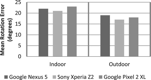
Due to the use of GNSS and its strong dependency on a line of sight (LOS), these systems are unreliable or even unusable for covered areas like street canyons, dense forests and especially buildings, in which the signals are obstructed (Blum, Greencorn, and Cooperstock 2013). Additionally, IMU of low-cost mobile devices are very susceptible to drift over time and lack precision in general, as described by Blum, Greencorn, and Cooperstock (2013). We also evaluated the IMU rotation accuracy of our three smartphones, the Google Nexus 5, the Sony Xperia Z2 and the Google Pixel 2 XL, and received similar results with mean rotation errors around 15–25°, as shown in Figure 1. For accurate AR visualizations, this is not feasible (see Figure 3).

Figure 1. Evaluation of the rotation error of three smartphones, the Google Nexus 5, the Sony Xperia Z2 and the Google Pixel 2 XL, in indoor and outdoor environments.

As a solution to GNSS and IMU unreliability, multiple stationary external pose tracking systems have been introduced, specifically for indoor environments; e.g. the ultrasound-based systems by Ward, Jones, and Hopper (1997) or Priyantha, Chakraborty, and Balakrishnan (2000), the commercial magnet-field system Polemus G4 or the commercial optical tracking systems SMARTTRACK3 and ARTTRACK5 by Advanced Realtime Tracking GmbH (ART). The disadvantages of these stationary external systems are their limited range and need of installment in the environment.

To maintain the flexibility of device-based pose tracking, cameras have found an increasing application for realizing optical pose tracking. For instance, White and Feiner (2009) include 6 degree of freedom optical marker tracking in SiteLens, for displaying virtual 3D building models. The fiducial markers are distributed across the environment and are captured by the mobile camera to provide known reference points for correcting the device pose. But like stationary external tracking systems, marker tracking also requires preparing the environment in advance, limiting the versatility of the AR systems. Therefore, efforts have been made to integrate existing physical objects, such as buildings, referred to as natural features, in optical pose tracking. Vacchetti, Lepetit, and Fua (2004), Wuest, Vial, and Stricker (2005), Reitmayr and Drummond (2006), Lima et al. (2010), Choi and Christensen (2012) and Petit, Marchand, and Kanani (2013) show virtual 3D model-based solutions using edge-matching methods. The defining edges of the 3D models are utilized to search for corresponding 2D edges of the physical objects in camera images and matched with these to derive a pose with the Perspective-n-Point (PnP) algorithm. Reitmayr and Drummond (2006) use their system to overlay virtual wireframe models over physical buildings. The drawbacks of these approaches are that the objects must be captured continuously by the camera to estimate poses, restricting mobility, and that, typically, prepared wireframe models are required.

In recent years, the increasing capabilities of low-cost off-the-shelf mobile devices have enabled AR systems to be implemented with smartphones. Multiple software frameworks like Vuforia (PTC), ARKit (Apple) or ARCore/Sceneform (Google), therefore, have been introduced, to realize AR on smartphones with readily available 3D real-time rendering and pose tracking. Primarily, the frameworks employ monocular visual-inertial odometry (VIO), a combination of single-camera natural feature and IMU tracking (Linowes and Babilinski 2017). The drawbacks of these frameworks are, on the one side, that pose estimation is only possible in a local reference frame, allowing only relative pose tracking, i.e. the poses are estimated relative to an arbitrary initial pose, and, on the other side, that there is no native support for CityGML, i.e. the data must be converted to a supported format like filmbox (FBX), with the risk of losing information in the process.

We introduce a more flexible custom pose tracking system that (1) can be utilized indoors and outdoors on off-the-shelf smartphones, (2) is fully self-contained and decoupled from external systems and (3) incorporates geometric-topologically and semantically rich CityGML data for the visualizations and the pose tracking in a global reference frame in parallel.

3 Mobile CityGML pose tracking system

To facilitate mobile self-contained indoor and outdoor tracking in a global reference frame, we integrate different pose tracking solutions in one system. In outdoor environments, GNSS, IMU and optical data, and in indoor environments, an indoor positioning system (IPS), as, for example, described by Real Ehrlich and Blankenbach (2019), IMU and optical data, are fused. The GNSS and IPS provide coarse positional information in the WGS84 global reference system and the IMU rotational information, global and local. For the global rotation, pitch and roll are determined with the accelerometer and yaw with the magnetometer, relative to magnetic north, and for the local rotation, accelerometer and gyroscope data are fused to determine yaw, pitch and roll. Each received pose is transformed into the CityGML data reference system, so pose and model information are in the same space.

The main component of the pose tracking system is the optical pose tracker. With a mobile CityGML database locally available on the AR device, as shown by Blut, Blut, and Blankenbach (2017), we can estimate poses in a global reference frame with the geo-referenced CityGML models. The basic principle of our optical pose estimation approach is to find 3D corners in the CityGML model and their corresponding 2D corners in camera images. The resulting pose is subsequently fused with the IMU data. The proof-of-concept pose tracking system was implemented with smartphones, since these provide all necessary components, such as GNSS receiver, IMU and camera, and using doors as pose estimation object, since these have an easily detectable simple geometric structure and are one of the basic objects of CityGML building models.

Two similar approaches to door-based pose estimation were presented by Händler (2012) for use in an IPS. The first solution uses fiducial markers with encoded object information placed on each door to identify them. The second solution employs an external database with images of each door, captured from various angles to account for differences in appearance, caused by the different viewpoints. To detect the doors, their contours are extracted from an image with the Canny algorithm (Canny 1986), to which a Hough transformation (Hough and Paul 1962) is applied. Once the door is found, a texturized image of the door is extracted, including distinctive door features, such as door handles. The texturized door candidates are then normalized and compared to the door images in the database. A disadvantage of these two methods is that they require preparations like placing fiducial markers or creating image databases in advance. Further issues are that a network connection is required and the total time for the pose estimation is ∼50 s, which is unsuitable for AR.

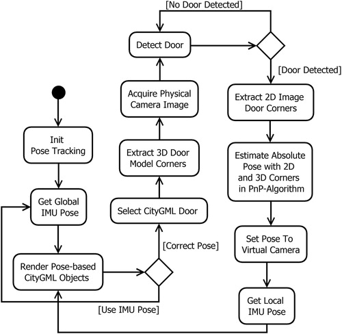
To realize real-time pose tracking with readily available data and hardware, we designed the system, as shown in Figure 2. The main challenges lie in the automated (1) extraction of 3D CityGML door corners, (2) extraction of 2D image door corners, and (3) pose estimation using corresponding 2D/3D door corners. These are described in the following subsections.

Figure 2. Activity diagram of the pose tracking system.

3.1 Three-dimensional corner extraction

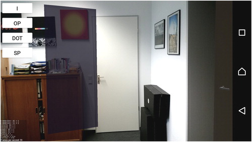
As shown in Figure 2, the first step after pose tracking initialization is to determine a coarse global pose, either from GNSS/IMU or IPS/IMU. Using the pose, the relevant CityGML objects are loaded from the local SpatiaLite database, according to Blut, Blut, and Blankenbach (2017) and rendered. Since pose tracking with the IMU is inaccurate (see Figure 1), the rendered CityGML objects do not align with their physical counterparts and appear shifted (see Figure 3).

Figure 3. Due to an inaccurate pose, the virtual CityGML door is shifted and does not align with the physical door.

To align the virtual and physical objects more accurately, the pose needs to be improved. For this, the user selects the door that should be used for the optical pose estimation. The selection determines the type of CityGML object and its identifier. Using this information and the topological and semantic model of CityGML, the corresponding database entry can quickly be found with the solution of Blut, Blut, and Blankenbach (2017), and the required geometry loaded. In the next step, the loaded geometry is processed to find the corners of the object, here the door. Since the door geometry typically consists of hundreds of points, a method is necessary to determine the corner points and sort them into a predefined order. This is done with the following steps:

1. Remove duplicate points.

2. Compute the bounding box of all points that belong to the door.

3. Sort the points from farthest to closest to the centre of the bounding box.

4. Save the 4 or 8 points farthest from the centre, as these most likely are the corner points of the door. If the door is modelled as a solid, it has 8 corner points and if it is modelled using only a surface, it has 4 corner points.

5. If the door is a surface, select the 4 corner points. If the door is a solid, select the 4 corner points that are closest to the camera, as these are the corner points of the surface visible to the user.

6. Sort the corner points counter-clock-wise.

The 3D corners are now ready to be used for the pose estimation. As shown in Figure 2, the corresponding 2D corners are next searched for in the camera image.

3.2 Two-dimensional corner extraction

The general idea for our 2D door corner extraction algorithm is to find best-fit corner candidates using a door detection algorithm based on the work of Yang and Tian (2010). The approach requires no training or preparations ahead of time and uses a geometric door model, an edge detector and a corner detector. The algorithm is independent of colour or texture information, so that a wide range of doors can be detected. The detection success heavily depends on the quality of the corners, since these are tested against the geometric door conditions. For this, Yang and Tian (2010) use a curvature-based corner detector. Alternatives are the Harris (Harris and Stephens 1988) corner detector or the Shi-Tomasi (Shi and Tomasi 1994) corner detector.

To identify the best method for our solution, the three corner detectors were evaluated in terms of corner quality (Table 1). Similar to Chen He and Yung (2008), some reference images were captured in which such corners were marked and noted manually that are generally regarded as corners by humans, thus, are at a right angle of two edges. In the following, these are referred to as true corners. The algorithms were run on 480 × 360 px images. In average, there were 51 true corners in the image set. The parameters of each algorithm were set, so that at least the door corners could be detected in the majority of the images.

Table 1. Comparison of corner detectors

Corner detector	Total found	Found true	Missed true	Found false	Included (%)
Harris	4243	37	14	4206	87
Shi-Tomasi	248	34	17	214	85
Curvature-based	319	34	17	285	89

As Table 1 shows, the Harris corner detector in average finds the most true corners, but on the downside also detects the most false corners, which are ∼20 times higher than with the Shi-Tomasi detector or curvature-based detector. This is crucial for the detection speed of the door detector, since larger corner numbers, generally, result in longer detection runtimes. Comparing the Shi-Tomasi detector to the curvature-based detector, the results are quite similar, with equal average found true corners and only slight differences in the amount of detected false corners. The Shi-Tomasi detector in average detects less false corners, which speaks for this solution, but the curvature-based detector showed better performance for the specific case of door detection, in which for 89% of the evaluation images the door corners were included. Therefore, the curvature-based detector was used for our implementation of the door detection algorithm.

The door detector proceeds as follows: before a search for edges and corners can be applied, the image is down-sampled to reduce computational cost. Gaussian blur is applied to remove noise. Next, a binary edge map is created using the Canny algorithm from which the contours are extracted. These contours are used for the corner detector based on Chen He and Yung (2008). The following steps consist of grouping the found corner candidates into groups of four according to the geometric model, which defines that a door consists of four corners $C_1,C_2,C_3,C_4$ and four edges $E_1,E_2,E_3,E_4$, and checking these against some geometric requirements such as that :

• a door must have a certain width and height,

• vertical edges should be parallel to each other,

• vertical edges are nearly perpendicular to the horizontal axis of the image.

To rate the width and height of a door, the relative size is calculated using the lengths of the door edges $E_{ij}$ and the length of the diagonal of the image $\mathrm{l}\mathrm{e}\mathrm{n}\mathrm{g}\mathrm{t}{\mathrm{h}}_{\mathrm{i}\mathrm{m}\mathrm{a}\mathrm{g}\mathrm{e}\mathrm{D}\mathrm{i}\mathrm{a}\mathrm{g}\mathrm{o}\mathrm{n}\mathrm{a}\mathrm{l}}$. The ratio is represented by the below equation(1) $\mathrm{S}\mathrm{i}{\mathrm{z}}_{ij}=\frac{\sqrt{{\left(x_i-x_j\right)}^2+{\left(y_i-y_j\right)}^2}}{\mathrm{l}\mathrm{e}\mathrm{n}\mathrm{g}\mathrm{t}{\mathrm{h}}_{\mathrm{i}\mathrm{m}\mathrm{a}\mathrm{g}\mathrm{e}\mathrm{D}\mathrm{i}\mathrm{a}\mathrm{g}\mathrm{o}\mathrm{n}\mathrm{a}\mathrm{l}}}$(1)

The orientation of the edges $E_{ij}$ is calculated using the below equation(2) $\mathrm{O}\mathrm{r}{\mathrm{i}}_{ij}=\mathrm{t}\mathrm{a}{\mathrm{n}}^{-1}\frac{\left|x_i-x_j\right|}{\left|y_i-y_j\right|}x\frac{180}{\pi }$(2)

The values are tested if these fall in a predefined threshold, set for each condition. Candidates that comply with the requirements are further tested by combining them with the edges found by the Canny algorithm. Edges of door candidates are checked if they match with the edge map by using a fill ratio which defines the amount that the edges overlap the edge map (below equation)(3) $\mathrm{F}{\mathrm{R}}_{ij}=\frac{\mathrm{O}\mathrm{v}\mathrm{e}\mathrm{r}\mathrm{L}\mathrm{a}{\mathrm{p}}_{ij}}{\mathrm{L}\mathrm{e}\mathrm{n}\mathrm{g}\mathrm{t}{\mathrm{h}}_{ij}}$(3) where $\mathrm{O}\mathrm{v}\mathrm{e}\mathrm{r}\mathrm{L}\mathrm{a}{\mathrm{p}}_{\mathit{i}j}$ is the length of the overlapping part of the edge and $\mathrm{L}\mathrm{e}\mathrm{n}\mathrm{g}\mathrm{t}{\mathrm{h}}_{ij}$ the total length of the edge $E_{ij}$.

In a last step, the 2D corner points are sorted counter-clock-wise, so these are in the same order as the 3D corners found in the previous step (Section 3.1).

3.3 Pose estimation with 2D/3D corners

Given 2D points (Section 3.2) in an image coordinate system extracted from an image and 3D object points (Section 3.1) in a world coordinate system extracted from CityGML data, we estimate a camera pose by exploiting the relationship between them. The relationship is expressed by the below equation:(4) $s{m}^{\mathrm{\prime }}=K\left(R|t\right)M^{\mathrm{\prime }},$(4) where $K\left(R|t\right)$ is the camera matrix that projects a 3D point $M^{\mathrm{\prime }}$ onto a 2D point $m^{\mathrm{\prime }}$ in a 2D plane and $s$ is an arbitrary scaling factor. $K$, the calibration matrix, contains the intrinsic parameters and $\left[R|t\right]$ the extrinsic parameters of the camera, where $R$ is the rotation matrix and $t$ the translation vector. Typically, pose tracking algorithms assume that $K$ is known and estimate $R$ and $t$.

The relationship between 2D and 3D points was already investigated nearly 180 years ago by Grunert (1841). The pose estimation approach is based on the observation that the angles between the 2D points are equal to the corresponding 3D points. A straightforward method was later introduced by Sutherland (1968) with the direct linear transformation (DLT) that can be used to estimate both the intrinsic and extrinsic camera parameters (see the below equation)(5) $\begin{array}{rl}& \frac{P_{11}{X}_i+P_{12}{Y}_i+P_{13}{Z}_i+P_{14}}{P_{31}{X}_i+P_{32}{Y}_i+P_{33}{Z}_i+P_{34}}=u_i,\\ & \frac{P_{21}{X}_i+P_{22}{Y}_i+P_{23}{Z}_i+P_{24}}{P_{31}{X}_i+P_{32}{Y}_i+P_{33}{Z}_i+P_{34}}=v_i.\end{array}$(5)

The equation can be solved using the singular value decomposition (SVD). The disadvantages of this solution are that a relatively high number of correspondences are necessary and that the results can be inaccurate (Faugeras 1993; Hartley and Zisserman 2004).

Therefore, more favourable solutions use a pre-determined camera calibration matrix $K$ so that instead of 11 parameters, only 6 must be estimated. Using $K$ and $n=3$ known correspondences generally is referred to as the perspective-three-point (P3P) problem. Many solutions to P3P have been introduced over the years, for example, Linnainmaa, Harwood, and Davis (1988), DeMenthon and Davis (1992), Gao et al. (2003) and Kneip, Scaramuzza, and Siegwart (2011). Typically, with $n=3$ known correspondences, four possible solutions are produced so that $n\ge 4$ correspondences are necessary for a unique solution. The $n\ge 4$ case is referred to as the PnP problem and, generally, is preferred, since the pose accuracy often can be increased with a higher number of points. Some PnP solutions were presented by Lepetit, Moreno-Noguer, and Fua (2009), Li, Xu, and Xie (2012), Garro, Crosilla, and Fusiello (2012) and Gao and Zhang (2013). Iterative solutions typically optimize a cost function based on error minimization, for example, using the Gauss–Newton algorithm (Gauß 1809) or the Levenberg–Marquardt algorithm (Levenberg 1944; Marquardt 1963). Examples are the minimization of the geometric error (e.g. 2D reprojection) or algebraic error. Some disadvantages of iterative solutions are that these require a good initial estimate. Noisy data strongly influence the results with the risk of falling into local minima. Also, the high computational complexity of many solutions renders them unusable for real-time applications. Therefore, an alternative to iterative solutions are non-iterative ones. A popular non-iterative PnP method is EPnP (Lepetit, Moreno-Noguer, and Fua 2009). The main idea is to represent the $n$ points of the 3D object space as a weighted sum of four virtual control points. The coordinates of the control points then can be estimated by expressing them as the weighted sum of the eigenvectors. Some quadric equations then are solved to determine the weights. An advantage of this approach is the $O\left(n\right)$ complexity.

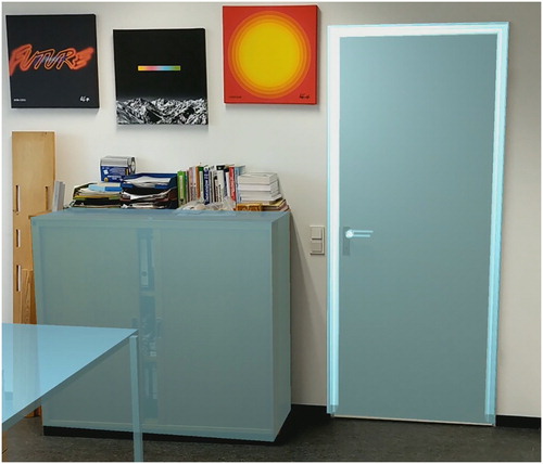
As shown in Figure 2, the received pose is utilized to correct the virtual camera and fused with accelerometer/gyroscope readings, to enable arbitrary rotations relative to the optical pose. Figure 4 shows an AR view with poses estimated with our pose tracking system. The virtual objects accurately overlay their physical counterparts.

Figure 4. AR view with poses estimated by our pose tracking system.

4 Evaluation

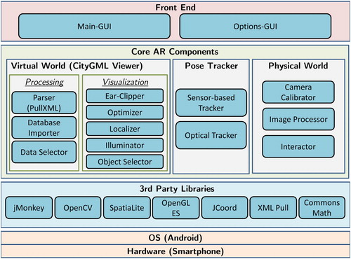
The introduced proof-of-concept pose tracking system was integrated into an Android-based AR system (Figure 5) and deployed to three smartphones, the Google Nexus 5, Sony Xperia Z2 and Google Pixel 2 XL, to evaluate its performance. For each smartphone, the system was calibrated to account for lens distortion effects of the smartphone cameras according to Luhmann et al. (2019).

Figure 5. Our AR system architecture. The entire system is Android-smartphone-based. The pose tracking system is one of three core AR components, and binds the physical and virtual world. All components utilize third party libraries, such as OpenCV, jMonkey and SpatiaLite. The system is accessible by the front-end graphical user interface.

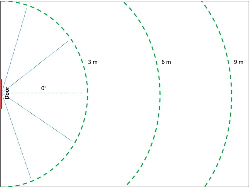
The pose tracking system was evaluated in terms of accuracy, runtime and stability, with an image dataset of various doors (Figure 6). Images were captured from distances of 3–9 m and at angles up to 70° in different lighting conditions, so that results can be summed up into the six measurement cases M1–M6, which represent our range of typical real-life application scenarios:

• M1: Near (3 m) straight

• M2: Far (up to 9 m) straight

• M3: Near (3 m) at angle

• M4: Far (up to 9 m) at angle

• M5: Good lighting

• M6: Bad lighting

Figure 6. Some examples of doors used for evaluating the optical pose estimation.

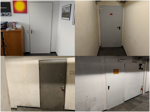
In total, 80 images that fit the cases (M1–M6) were captured with each smartphone. Most images contained a door in a complex scene. We define complex scenes as cluttered environments with arbitrary objects such as wall paintings, books or other furniture. Additionally, 20 images with no door, but some similar objects such as pictures on walls, were added to the dataset. For M1 and M2, the camera was placed straight towards the door at different distances, for M3 and M4, the camera was placed next to the door, at an angle. For good lighting conditions (M5), images were captured during the day. Indoors, the windows were fully opened, and artificial lighting was turned on. For bad lighting conditions (M6), images were captured on an overcast day with the blinds of the windows shut and all artificial lighting turned off. Figure 7 shows the used evaluation set-up.

Figure 7. Set-up for evaluating the optical pose estimation.

In the following sections, we present the evaluation results of the door detection, the pose estimation and the pose fusion, since these are the key components of our pose tracking system; therefore, the evaluation also reflects the practical applicability of our solution.

4.1 Door detection

The pose tracking depends on the performant, reliable and accurate detection of doors. To find a balance between these factors, we evaluated the detection runtime and rate with different image resolutions. The detection rate was calculated by classifying the detection results into four different cases:

• The image contains a door and the door was properly detected (true positive – TP) (Figure 8).

• The image contains a door, but the door was not detected (false negative – FN) (Figure 9).

• The image contains no door and no door was detected (true negative – TN).

• The image contains no door, but a door was detected (false positive – FP).

Figure 8. Example of the detected door. The red dots are corner points and the green rectangle is the correctly detected door.

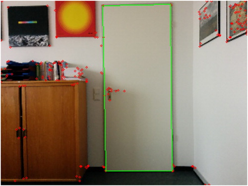
Figure 9. Example of a partially detected door.

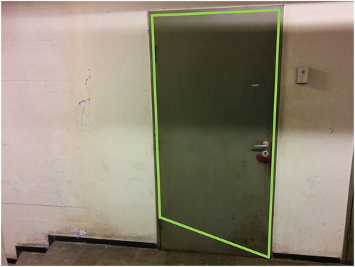
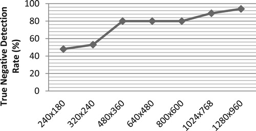
Figure 10 shows the success rate (TP) of detecting a door in images at different resolutions containing a door and Figure 11 the success rate of determining that no door is included in images (TN) at different resolutions. As Figure 10 depicts, with a resolution of 240 × 180 px, the algorithm only has a TP detection rate of 19% and increases rapidly to more than four times as much with a resolution of 480 × 360 px. Higher resolutions only slightly improve the TP rate. A similar trend is found for the TN rate (Figure 11). With a resolution of 240 × 180 px, in more than 50%, a door is falsely detected in an image without a door. For 480 × 360 px images, the rate is reduced to 20% (80% TN rate) and only increases slightly for higher resolution images.

Figure 10. True positive detection rate of the door detection algorithm for images with different resolutions.

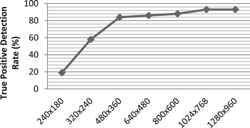
Figure 11. True negative detection rate of the door detection algorithm for images with different resolutions.

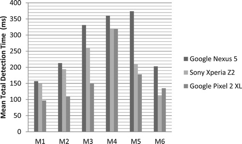
The measured detection time is defined as the duration of the entire detection process, including steps such as downscaling of the image, extracting edges and analysing these. Figure 12 shows the mean time required to detect a door in images with different resolutions. The total detection time is lowest for 240 × 180 px with 17 ms for the Google Pixel 2 XL, 56 ms for the Sony Xperia Z2 and 72 ms for the Google Nexus 5 and increases with the size of the images to 1.5 s for the Google Pixel 2 XL, 3.5 s for the Sony Xperia Z2 and 5.1 s for the Google Nexus 5.

Figure 12. Time required to detect a door in cases using the same images in different resolutions.

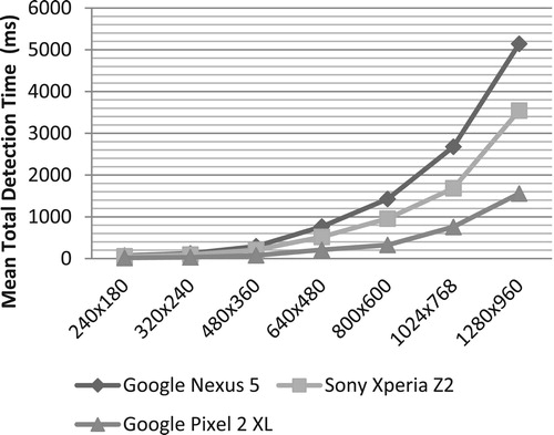
Generally, we found that a resolution of 480 × 360 px represents the best compromise between detection rate (Figures 10 and 11) and runtime (Figure 12). We, therefore, based our further evaluations, specifically M1–M6, on this resolution.

We found that the TP detection rate of 84% is independent of the cases M1–M6, but the mean detection time varies. As Figure 13 shows, the time does not directly correlate with the distance, angle or lighting, but with the background of the door. Backgrounds with various different colours and shapes increase the required detection time, since the algorithm finds more potential corners in such cluttered backgrounds. Therefore, doors that are surrounded by objects require more time compared to doors that are only surrounded by white walls. Typically, the images captured at an angle and from a distance contained more of the surrounding environment, so that the detection process was more complex.

Figure 13. Time required to detect a door in cases M1–M6 with 480 × 360 px images.

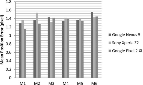
The accuracy of the detection algorithm describes how well the automatically derived corners match the actual corners of the door. A good accuracy is crucial for accurate pose estimations, as shown by Händler (2012). For this, the door corners were manually extracted from each image and the automatically derived corners were compared to them. Figure 14 shows that the automatically extracted door corners of our algorithm in average only lie 1.3 px from the reference corners, which is sufficient for accurate optical pose estimation.

Figure 14. Accuracy of the automatically derived door corners with 480 × 360 px images.

4.2 Optical pose estimation

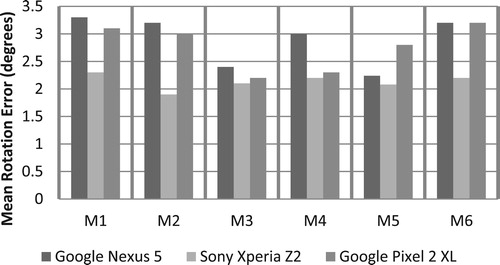
When using images to estimate poses, factors such as the distance or angle to the object (e.g. door) and lighting conditions potentially influence the accuracy of the pose. To confirm or refute this, poses were estimated for the cases M1–M6 and the accuracy of the automatically estimated poses was determined by comparing them to manually calculated reference poses. Figure 15 shows the positional differences and Figure 16 the angular differences. Generally, the automatic pose estimations in average lie 17 cm from the reference position and 2.5° in average from the reference rotation. The results show that the accuracy is generally independent from the angle, distance or the lighting conditions.

Figure 15. Accuracy of automatically estimated position.

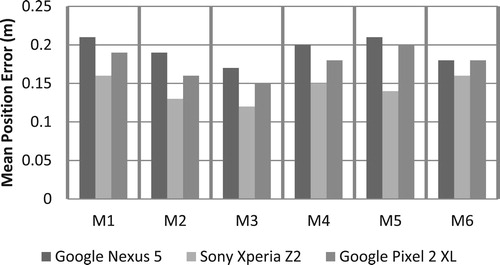
Figure 16. Accuracy of automatically estimated orientation.

4.3 Fusing optical and IMU poses

Given an initial pose from our optical pose system, fused local IMU poses enable the user to freely look around. The stability of these poses is essential for the pose tracking system. This is inspected by measuring the influence of sensor drift and the impact of relative movements. The stability of the augmentations was analysed using three different sensor types provided by the Android smartphones, the Rotation Vector, the Game Rotation Vector and the gyroscope. The Rotation Vector and Game Rotation Vector are referred to as composite sensors (Google, 10 December 2019, https://developer.android.com/guide/topics/sensors), since they use multiple hardware sensors and apply sensor fusion. The Rotation Vector incorporates the accelerometer, magnetometer and gyroscope and reports the rotation relative to magnetic north. The Game Rotation Vector utilizes the accelerometer and gyroscope and measures relative to an arbitrary starting point, like the gyroscope.

Two cases were evaluated, first, the impact of the sensor drift on pose tracking, secondly, the impact of device movements, for example, when the user looks around. For both cases, the difference between the initial and end pose was determined. For the resting AR system, each smartphone was placed in a stable pose using a sturdy tripod. The initial pose was automatically saved after a delay of 2 s to prevent any distortions caused by interactions with the touch screen. After a pre-determined amount of time, the next pose was saved and compared to the initial pose. The resulting rotation errors for each smartphone and the different sensor types are shown in Figures 17–19, respectively.

Figure 17. Quality of relative rotation over time using the rotation vector.

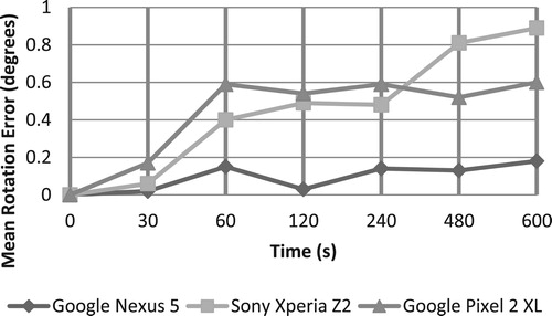
Figure 18. Quality of relative rotation over time using the game rotation vector.

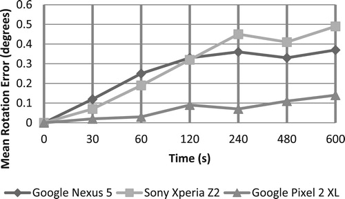
Figure 19. Quality of relative rotation over time using the gyroscope.

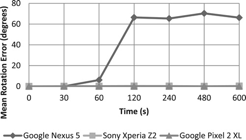
Figure 17 shows that the Rotation Vectors, generally, perform well in a 10 min window, with the mean rotation errors below 1°. While the error of the Google Nexus 5 increases the slowest, the Sony Xperia Z2 shows a rather steep linear increase. The curve of the Google Pixel 2 XL shows that the error stabilizes after a certain time. The Game Rotation Vectors (Figure 18) show the mean rotation errors under 0.5° in a 10 min window. The Google Pixel 2 XL performs the best but shows a linear error increase. In comparison, the errors of the Google Nexus 5 and the Sony Xperia Z2 each stabilize after a certain time. While the average absolute rotation from the Rotation Vector suffers from the inaccurate measurements of the magnetometer resulting in bearing errors up to 25° [also see (Schall et al. 2009)], the relative rotation results are significantly better. A comparison of Figures 17 and 18 with Figure 19 shows that the quality of the rotation benefits from sensor fusion in the Rotation Vector and Game Rotation Vector. While the rotation derived from the gyroscope (Figure 19) alone is comparatively good for the Sony Xperia Z2 and Google Pixel 2 XL, the Google Nexus 5 suffers significantly from the sensor drift

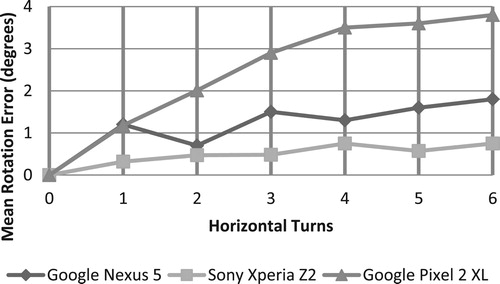
The impact of movement was evaluated by comparing the initial pose to the pose after the movements. To find the exact physical pose, the device was in before being moved, a tripod was used of which the initial pose was marked on the corresponding surface. The entire tripod with the smartphone then was moved accordingly and later placed exactly in the markings again. The results for each smartphone and type of sensor are displayed in Figures 20–22, respectively. Figure 20 shows that the mean rotation error is not influenced by movement when using the Rotation Vector. Figures 21 and 22 show that the mean rotation error increases with each turn when using the Game Rotation Vector and gyroscope. In both cases, the Sony Xperia Z2 shows the best and the Google Pixel 2 XL the poorest results.

Figure 20. Quality of relative rotation using the rotation vector when AR system is rotated.

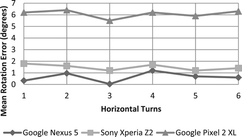
Figure 21. Quality of relative rotation using the game rotation vector when AR system is rotated.

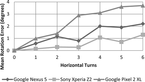
Figure 22. Quality of relative rotation using the gyroscope when AR system is rotated.

5 Conclusions and future work

The evaluation shows that low-cost off-the-shelf mobile devices, such as smartphones, are sufficient to realize a performant mobile AR pose tracking system with CityGML data, independent of exterior infrastructures. The introduced optical pose tracking method is real time capable and provides accurate results, enabling AR use cases as described in Section 1. Additionally, with CityGML-based pose tracking, the poses become tightly coupled to the model data. This not only allows geo-referenced visualizations of model data, but also, for example, extending models with newly captured geo-referenced information. For instance, damaged areas could be documented, building parts annotated or even missing models added.

The performance especially benefits from newer generation smartphones, such as the Google Pixel 2 XL. The fusion of the optical pose with local IMU poses allows the user to freely look around. The low-cost sensors of the evaluation smartphones provide sufficient results, but the pose tracking could be further improved. Currently, the door detection relies on features found by a corner detector. The entirety of points is analysed and tested against selected conditions to find possible door candidates. While the current implementation already provides good results with a detection speed of 215 ms and a positive detection rate of 80%, the detection rate could still be improved by increasing the image resolution, which would increase feature detectability, at the cost of detection speed. To counter this, the amount of corner points could be reduced by additional conditions. An approach could be to exploit the colour of the doors. This information is available in the CityGML model, so an additional test could be performed to check if the found corner points are part of a certain coloured CityGML object.

The initial pose derived from the door-based pose estimation in average has a positional accuracy of 17 cm and a rotation accuracy of 2.5°. The following relative IMU pose tracking in average has a rotation error of 1–6°. This is noticeable in the visual augmentations, but not a major issue, since the virtual objects augment their physical counterparts sufficiently for the AR use cases described in Section 1. To further increase the quality of the augmentations and stabilize them, a possibility would be to combine edge-based pose tracking, as shown by Reitmayr and Drummond (2006), and our door-based method. Since the edge-based solution requires a good initial pose, our door detection solution could be utilized for initialization. The disadvantage here would be that the door must always be visible for the edges to be matched. Therefore, the solution would need to be extended to use other objects in the vicinity. A challenge hereby would be to find reliable physical objects, which, on the one hand, have a constant pose over time and, on the other hand, do not have an overly complex shape to be detected reliably.

Alternatively, VIO, as, for example, in ARCore, could be effective. As described by Google (10 December 2019, https://developers.google.com/ar/discover/concepts), ARCore finds unambiguously re-identifiable image features and tracks these across subsequent images, deriving a relative camera motion. The resulting poses are fused with IMU data. Additionally, ARCore uses the sets of detected features to find and derive planes, such as wall-, ceiling-, floor- or table surfaces. These planes could be utilized for a geometry matching process with the corresponding geo-referenced CityGML surfaces, to obtain poses in a global reference frame. Disadvantageous is that the plane detection relies on image features, so that flat surfaces must be sufficiently texturized. White walls, therefore, may not be detectable for example.

Disclosure statement

No potential conflict of interest was reported by the author(s).

References

- Agugiaro, Giorgio, Joachim Benner, Piergiorgio Cipriano, and Romain Nouvel. 2018. “The Energy Application Domain Extension for CityGML: Enhancing Interoperability for Urban Energy Simulations.” Open Geospatial Data, Software and Standards 3 (1). doi: 10.1186/s40965-018-0042-y.
- Biljecki, Filip, Kavisha Kumar, and Claus Nagel. 2018. “CityGML Application Domain Extension (ADE): Overview of Developments.” Open Geospatial Data, Software and Standards 3 (1): 1–17. doi:10.1186/s40965-018-0055-6.
- Biljecki, Filip, Jantien Stoter, Hugo Ledoux, Sisi Zlatanova, and Arzu Çöltekin. 2015. “Applications of 3D City Models: State of the Art Review.” ISPRS International Journal of Geo-Information 4 (4): 2842–2889. doi:10.3390/ijgi4042842.
- Blum, Jeffrey R., Daniel G. Greencorn, and Jeremy R. Cooperstock. 2013. “Smartphone Sensor Reliability for Augmented Reality Applications.” doi:10.1007/978-3-642-40238-8_11.
- Blut, Christoph, Timothy Blut, and Jörg Blankenbach. 2017. “CityGML Goes Mobile: Application of Large 3D CityGML Models on Smartphones.” International Journal of Digital Earth, 1–18. doi:10.1080/17538947.2017.1404150.
- Canny, John. 1986. “A Computational Approach to Edge Detection.” IEEE Transactions on Pattern Analysis and Machine Intelligence (6): 679–698. doi:10.1109/TPAMI.1986.4767851.
- Chen He, Xiao, and Nelson Hon Ching Yung. 2008. “Corner Detector Based on Global and Local Curvature Properties.” Optical Engineering 47 (5). doi:10.1117/1.2931681.
- Choi, Changhyun, and Henrik I Christensen. 2012. “3D Textureless Object Detection and Tracking an Edge Based Approach.” IEEE/RSJ International Conference on Intelligent Robots and Systems (IROS), 3877–3884. doi:10.1109/IROS.2012.6386065.
- DeMenthon, Daniel F., and Larry S. Davis. 1992. “Model-Based Object Pose in 25 Lines of Code.” In European Conference on Computer Vision, 335–343. Springer. doi:10.1007/3-540-55426-2_38.
- Faugeras, Oliver. 1993. Three-Dimensional Computer Vision: A Geometric Viewpoint. MIT Press. doi:10.1007/978-3-642-82429-6_2.
- Feiner, Steven, Blair Macintyre, Tobias Höllerer, and Anthony Webster. 1997. “A Touring Machine: Prototyping 3D Mobile Augmented Reality Systems for Exploring the Urban Environment.” In ISWC ‘97. Cambridge, MA, USA, 1, 74–81.
- Gao, Xiao Shan, Xiao Rong Hou, Jianliang Tang, and Hang Fei Cheng. 2003. “Complete Solution Classification for the Perspective-Three-Point Problem.” IEEE Transactions on Pattern Analysis and Machine Intelligence 25 (8): 930–943. doi:10.1109/TPAMI.2003.1217599.
- Gao, Jingyi, and Yalin Zhang. 2013. “An Improved Iterative Solution to the PnP Problem.” Proceedings - 2013 International Conference on Virtual Reality and Visualization, ICVRV 2013, no. 3, 217–220. doi:10.1109/ICVRV.2013.41.
- Garro, Valeria, Fabio Crosilla, and Andrea Fusiello. 2012. “Solving the PnP Problem with Anisotropic Orthogonal Procrustes Analysis.” Second International Conference on 3D Imaging, Modeling, Processing, Visualization Transmission, IEEE, 262–269. doi:10.1109/3DIMPVT.2012.40.
- Gauß, Carl Friedrich. 1809. “Theoria Motus Corporum Coelestium in Sectionibus Conicis Solem Ambientium.” Hamburgi: Sumtibus Frid. Perthes et I. H. Besser. doi:10.3931/e-rara-522.
- Gröger, Gerhard, Thomas Kolbe, Claus Nagel, and Karl-Heinz Häfele. 2012. “OGC City Geography Markup Language (CityGML) En-Coding Standard.” OGC, 1–344. doi:OGC 12-019.
- Grunert, Johann August. 1841. “Das Pothenotische Problem in Erweiterter Gestalt Über Seine Anwendungen in Der Geodäsie.” In Archiv Der Mathematik Und Physik, Band 1, 238–248. Greifswald: Verlag von C. A. Koch.
- Händler, Verena. 2012. Konzeption Eines Bildbasierten Sensorsystems Zur 3D- Indoorpositionierung Sowie Analyse Möglicher Anwendungen. Fachrichtung Geodäsie Fachbereich Bauingenieurwesen und Geodäsie Technische Universität Darmstadt.
- Harris, Chris, and Mike Stephens. 1988. “A Combined Corner and Edge Detector.” In Proc. of Fourth Alvey Vision Conference. http://citeseerx.ist.psu.edu/viewdoc/download?doi=10.1.1.434.4816&rep=rep1&type=pdf.
- Hartley, Richard, and Andrew Zisserman. 2004. Multiple View Geometry in Computer Vision. 2nd ed. Cambridge University Press. doi:10.1016/S0143-8166(01)00145-2.
- Herbert, Grant, and Xuwei Chen. 2015. “A Comparison of Usefulness of 2D and 3D Representations of Urban Planning.” Cartography and Geographic Information Science. doi:10.1080/15230406.2014.987694.
- Hollerer, T., S. Feiner, and J. Pavlik. 1999. “Situated Documentaries: Embedding Multimedia Presentations in the Real World.” In ISWC ‘99, 99, 79–86. San Francisco, CA: IEEE. doi:10.1109/ISWC.1999.806664.
- Hough, V., and C. Paul. 1962. Method and Means for Recognizing Complex Patterns. 3069654, issued 1962. doi:10.1007/s10811-008-9353-1.
- Kneip, Laurent, Davide Scaramuzza, and Roland Siegwart. 2011. “A Novel Parametrization of the Perspective-Three-Point Problem for a Direct Computation of Absolute Camera Position and Orientation.” Proceedings of the IEEE Computer Society Conference on Computer Vision and Pattern Recognition, 2969–2976. doi:10.1109/CVPR.2011.5995464.
- Lepetit, Vincent, Francesc Moreno-Noguer, and Pascal Fua. 2009. “EPnP: An Accurate O(n) Solution to the PnP Problem.” International Journal of Computer Vision 81 (2): 155–166. doi:10.1007/s11263-008-0152-6.
- Levenberg, Kenneth. 1944. “A Method for the Solution of Certain Non-Linear Problems in Least Squares.” Quarterly of Applied Mathematics 2 (2): 164–168. doi:10.1090/qam/10666.
- Li, Shiqi, Chi Xu, and Ming Xie. 2012. “A Robust O(n) Solution to the Perspective-n-Point Problem.” IEEE Transactions on Pattern Analysis and Machine Intelligence 34 (7): 1444–1450. doi:10.1109/TPAMI.2012.41.
- Lima, João Paulo, Francisco Simões, Lucas Figueiredo, and Judith Kelner. 2010. “Model Based Markerless 3D Tracking Applied to Augmented Reality.” Journal on 3D Interactive Systems 1: 2–15. ISSN: 2236-3297.
- Linnainmaa, Seppo, David Harwood, and Larry S. Davis. 1988. “Pose Determination of a Three-Dimensional Object Using Triangle Pairs.” IEEE Transactions on Pattern Analysis and Machine Intelligence 10 (5): 634–647. doi:10.1109/34.6772.
- Linowes, Jonathan, and Krystian Babilinski. 2017. Augmented Reality for Developers: Build Practical Augmented Reality Applications with Unity, ARCore, ARKit, and Vuforia. Birmingham: Packt Publishing Ltd.
- Luhmann, Thomas, Stuart Robson, Stephen Kyle, and Jan Boehm. 2019. Close-Range Photogrammetry and 3D Imaging. doi:10.1515/9783110607253.
- Marquardt, Donald W. 1963. “An Algorithm for Least-Squares Estimation of Nonlinear Parameters.” Journal of the Society for Industrial and Applied Mathematics 11 (2): 431–441. doi: 10.1137/0111030. doi: 10.1137/0111030
- Petit, Antoine, Eric Marchand, and Keyvan Kanani. 2013. “A Robust Model-Based Tracker Combining Geometrical and Color Edge Information.” IEEE International Conference on Intelligent Robots and systems, IEEE, 3719–3724. doi:10.1109/IROS.2013.6696887.
- Piekarski, Wayne, and Bruce Thomas. 2001. “Augmented Reality with Wearable Computers Running Linux.” 2nd Australian Linux Conference (Sydney), 1–14.
- Priyantha, Nissanka B, Anit Chakraborty, and Hari Balakrishnan. 2000. “The Cricket Location-Support System.” Proceedings of the 6th Annual International Conference on Mobile Computing and Networking, 32–43. doi:10.1145/345910.345917.
- Real Ehrlich, Catia, and Jörg Blankenbach. 2019. “Indoor Localization for Pedestrians with Real-Time Capability Using Multi-Sensor Smartphones.” Geo-Spatial Information Science 22 (2): 73–88. doi:10.1080/10095020.2019.1613778.
- Reitmayr, Gerhard, and Tom W. Drummond. 2006. “Going Out: Robust Model-Based Tracking for Outdoor Augmented Reality.” Proceedings of the 5th IEEE and ACM International Symposium on Mixed and Augmented reality, IEEE, 109–118. doi:10.1109/ISMAR.2006.297801.
- Santana, José Miguel, Jochen Wendel, Agustín Trujillo, José Pablo Suárez, Alexander Simons, and Andreas Koch. 2017. “Multimodal Location Based Services – Semantic 3D City Data as Virtual and Augmented Reality.” In Progress in Location-Based Services 2016, 329–353. Springer. doi:10.1007/978-3-319-47289-8_17.
- Schall, Gerhard, Dieter Schmalstieg, and Sebastian Junghanns. 2010. “Vidente – 3D Visualization of Underground Infrastructure Using Handheld Augmented Reality.” GeoHydroinformatics: Integrating GIS and Water, 207–219. doi:10.1.1.173.3513.
- Schall, Gerhard, Johannes Schöning, Volker Paelke, and Georg Gartner. 2011. “A Survey on Augmented Maps and Environments: Approaches, Interactions and Applications.” Advances in Web-Based GIS, Mapping Services and Applications 9: 207–225. doi: 10.1201/b11080-18
- Schall, G., D. Wagner, G. Reitmayr, E. Taichmann, M. Wieser, D. Schmalstieg, and B. Hofmann-Wellenhof. 2009. “Global Pose Estimation Using Multi-Sensor Fusion for Outdoor Augmented Reality.” 8th IEEE International Symposium on Mixed and Augmented reality, IEEE, 153–162. http://ieeexplore.ieee.org/xpls/abs_all.jsp?arnumber=5336489%5Cnpapers2://publication/uuid/0F6141AD-F7D5-476E-93F0-425FC456B02F.
- Schmalstieg, Dieter, and Tobias Höllerer. 2016. Augmented Reality – Principles and Practice. Boston, MA: Addison-Wesley Professional.
- Shi, Jianbo, and Carlo Tomasi. 1994. “Good Features to Track.” Proceedings of IEEE Conference on Computer Vision and Pattern Recognition, 593–600. doi:10.1109/CVPR.1994.323794.
- Stylianidis, E., E. Valari, K. Smagas, A. Pagani, J. Henriques, A. Garca, E. Jimeno, et al. 2016. “LARA: A Location-based and Augmented Reality Assistive System for Underground Utilities’ Networks Through GNSS.” Proceedings of the 2016 International Conference on Virtual Systems and Multimedia, IEEE, 1–9. doi:10.1109/VSMM.2016.7863170.
- Sutherland, Ivan E. 1968. “A Head-Mounted Three Dimensional Display.” Proceedings of the December 9–11, 1968, Fall Joint Computer Conference, Part I on – AFIPS ‘68 (fall, part I), San Francisco, CA, 757–764. doi:10.1145/1476589.1476686.
- Vacchetti, Luca, Vincent Lepetit, and Pascal Fua. 2004. “Combining Edge and Texture Information for Real-Time Accurate 3D Camera Tracking.” Proceedings of the Third IEEE and ACM International Symposium on Mixed and Augmented Reality (ISMAR 2004), IEEE, 48–56. doi:10.1109/ISMAR.2004.24.
- Ward, Andy, Alan Jones, and Andy Hopper. 1997. “A New Location Technique for the Active Office.” IEEE Personal Communications 4 (5): 42–47. doi:10.1109/98.626982.
- White, Sean, and Steven Feiner. 2009. “SiteLens: Situated Visualization Techniques for Urban Site Visits.” Proceedings of the SIGCHI Conference on Human factors in Computing Systems, Boston, MA, USA, ACM, 1117–1120. doi:10.1145/1518701.1518871.
- Wuest, Harald, Florent Vial, and Didier Stricker. 2005. “Adaptive Line Tracking with Multiple Hypotheses for Augmented Reality.” Proceedings – Fourth IEEE and ACM International Symposium on Symposium on Mixed and Augmented Reality, ISMAR 2005, IEEE Computer Society, 62–69. doi:10.1109/ISMAR.2005.8.
- Yang, Xiaodong, and Yingli Tian. 2010. “Robust Door Detection in Unfamiliar Environments by Combining Edge and Corner Features.” 2010 IEEE Computer Society Conference on Computer Vision and Pattern Recognition – Workshops, CVPRW 2010, IEEE, 57–64. doi:10.1109/CVPRW.2010.5543830.