Distinguishing different subclasses of water bodies for long-term and large-scale statistics of lakes: a case study of the Yangtze River basin from 2008 to 2018

ABSTRACT

Long-term and large-scale lake statistics are meaningful for the study of environment change, but many of the existing methods are labour-intensive and time-consuming. To overcome this problem, a novel method for long-term and large-scale lake extraction by shape-factors- and machine-learning-based water body classification is proposed. An experiment was conducted to extract the lakes in the Yangtze River basin (YRB) from 2008 to 2018 with the Joint Research Centre's Global Surface Water Dataset (JRC GSW) data and OSM data. The results show: 1) The proposed method is automatically and successfully executed. 2) The number of river–lake complexes is between 3008 and 4697, representing 3.56%–5.70% of the total water bodies. 3) The areas of the lakes and rivers in the YRB were obtained, and the accuracy of water classification in each year was stable between 90.2% and 93.6%. Comparing the back propagation neural network, random forest, and support vector machine models, we found that the three machine learning models have similar classification accuracy for the scenario. 4) Fragmented and incomplete small rivers in the JRC GSW data, unchecked training samples, and overlapped shape factors are the three error sources. Future work will focus on addressing these three error sources.

KEYWORDS:

• Lake extraction
• water bodies classification
• the Yangtze River
• shape metrics
• machine learning

1. Introduction

Lakes play an important role in the environment. Spatiotemporal change analysis of lakes in a basin, in a continent, and even on the global scale reflects the impact of climate change and human activities on the environment, with long-term and large-scale lake extraction as the basis (Qiao, Zhu, and Yang 2019; Wang, Sheng, and Tong 2014; Yao et al. 2019; Zhang et al. 2019). With the accumulation of massive remote sensing data (Ma et al. 2015) and the development of water extraction technology, methods of water bodies extraction were proposed and the global water bodies databases were established (Chen et al. 2015; Lehner and Döll 2004; Pekel et al. 2016). The methods for specific lake extraction from remotely sensed data are mature to some extent (Pekel et al. 2016), but an effective method for long-term and large-scale lake extraction is lacking. Therefore, extracting long-term and large-scale lakes from water bodies, which involves a process of distinguishing different subclasses of water bodies, is required. Water body classification methods could be roughly divided into three types: visual interpretation, historical data, and shape factor methods.

The visual interpretation method is widely used in water classification (Wang, Sheng, and Tong 2014; Yao et al. 2019), and its accuracy is high. However, visual interpretation is labour-intensive. Long-term and large-scale visual interpretation may require a large amount of human resources. For example, at least 516 images need to be interpreted visually to classify the water bodies in China for one year (Zhang et al. 2019). Visual interpretation relies on the operators’ subjective experience and knowledge; thus, different operators have different understandings, which affects the reliability of the results.

In the historical data method, the lakes are separated from other water bodies according to historical data (Zhang et al. 2019; Xie et al. 2017). The method is based on the assumption that the distributions of the lakes in the study area has not changed or the changes can be ignored. However, water bodies are always changing. When the period between the reference historical data and the research data is long, the method may considerably deviate from the actual classification results. The appropriate historical data with fine resolution and good quality in the same study area may be hard to find. The historical data may be derived from the results of visual interpretation.

The shape factor method completes the classification of water body based on the differences in morphology of the different water body subclasses. In some studies, one to three shape factor formulas were used to quantify the differences among different water subcategories (Jiao, Liu, and Li 2012; van der Werff and van der Meer 2008), and the researcher provides a threshold to distinguish lakes from other water bodies (Jiao, Liu, and Li 2012). In the shape factor method, the classification threshold must be set manually. Each shape factor is designed for a specific purpose, which makes it unsuitable for measuring the morphological differences of water subclasses. That is, a few shape factors may not always reflect the morphological differences of different water subclasses (Feyisa et al. 2014; Fisher, Flood, and Danaher 2016; Huang et al. 2018; Khandelwal et al. 2017). In addition, manually setting thresholds may cause serious misclassification.

These three types of water body classification methods are labour-intensive or require manual intervention, so are unsuited for long-term and large-scale lake extraction. An automatic water body classification method is needed. Although the shape factor method cannot satisfy the requirements, its idea is worth applying. The shape factor method involves quantifying the morphological differences of various water bodies using a formula, and separation thresholds are set to finish water classification. After careful study, three issues with the shape factor method should be improved. Firstly, river–lake complexes need to be disassembled, which affects the results of classification but was ignored or manual dismantling was required in previous papers (Downing et al. 2012; Lehner and Döll 2004). Secondly, special shape factors should be considered because the existing water classification studies often applied a low number of shape factors. Third, manually determining the threshold should be avoided to eliminated the need for manual intervention. As it has been widely used in the classification of land cover, machine learning is one of the best choices for object classification (Talukdar et al. 2020). Machine learning can be used for reference. Automatic sampling for machine learning is also vital. Hence, the potential of volunteered geographic information (VGI) (Goodchild 2007) for automatic sampling was explored in this study.

The objective of this study was to construct a method to distinguish different subclasses of water bodies for long-term and large-scale lake statistics. We selected the Yangtze River basin, China, as study area and the Joint Research Centre's Global Surface Water (JRC GSW) dataset from 2008 to 2018 to demonstrate the accuracy of the proposed method. The contributions of the study are (1) a method to distinguish subclasses of water bodies for long-term and large-scale lake extraction based on shape factors and machine learning, (2) a separation method of river–lake complexes, and (3) extraction of the lakes from 2008 to 2018 in the Yangtze River basin, China.

2. Study area and data

2.1. Study area

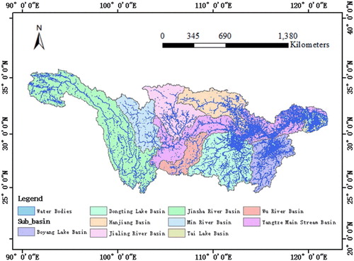
The Yangtze River basin, as shown in Figure 1, is the largest basin in China, with a total area of 180 km². The average annual precipitation of the Yangtze River basin is 1067 mm. The Yangtze River basin is the most densely distributed area of freshwater resources in China (Jiang, Su, and Hartmann 2007), with thousands of lakes and a large number of river–lake complexes. The basin is high in the west and low in the east, and the terrain varies. The terrain mainly includes plateaus, mountains, hills, and plains. Due to the variety of terrain, the lake shapes in the basin differ. As one of the busiest areas of human activity, the Yangtze River basin has a population of 400 million and produces more than 40% of China's GDP. The impact of human activities on lakes and rivers has increasingly attracted scholars’ attention (Guo et al. 2012). Many scholars started from the changes in the number and area of lakes to quantifying the impact of human activities. Therefore, the Yangtze River basin was a suitable experimental area to verify the proposed water classification method.

Figure 1. The location of the Yangtze River basin.

2.2. Data

2.2.1. JRC GSW

The JRC GSW (Pekel et al. 2016) dataset is a database recording the global surface water bodies from 1984 to 2018, providing the global water body distribution over the 32 years. The spatial resolution of the water body data is up to 30 metres and the average extracted accuracy is more than 95%. The water database has a long time span, continuously recording the whole spherical surface water body for 32 years, which meets our long-term data requirement for this experiment. The database can be downloaded for free from the Google Earth Engine platform (GEE). We selected the yearly maximum surface water from 2008 to 2018 as the experimental data.

2.2.2. Volunteered geographic information (VGI)

VGI, a new source of geographic information, has become available in the form of user-generated web content (Rana and Joliveau 2009). As some of the most popular VGI data, OpenStreetMap (OSM) data are used as the data source of samples in many studies (Ballatore, Bertolotto, and Wilson 2013; Neis, Zielstra, and Zipf 2012). Our two main reasons for using OSM data in this study were: OSM data can be obtained online free of charge, and the water layer of OSM contains information for many water subclasses. The water layer provides the spatial distribution information of water polygons, and the water subclass and name of each water polygon. The water subclass information of each water body is provided by ‘fclass’, and the name of each water body is provided by ‘name’. Fclass divides water bodies into six subcategories: water, reservoir, river, dock, glacier, and wetland. The specific descriptions of these six subcategories are provided in Table 1. Name records the real names of water bodies. Because the research area is located in China, most of the names of water bodies are recorded in Chinese, and a small number of names of water bodies are recorded in English or other languages.

Table 1. Six subcategories of water bodies in Open Street Map (OSM).

fClass	Description
Water	Unspecified bodies of water. Typically lakes, but can also be larger rivers, harbours, etc.
Reservoir	Artificial lakes, typically above a dam.
River	Polygons for larger rivers.
Dock	Dock (to repair ships, don't confuse it with the American term “dock”)
Glacier	Glaciers
Wetland	Swamp, bog, or marsh land

Different countries and research institutions often divide water bodies into different types with different standards. In this study, we needed to separate other water bodies from lakes. Therefore, we divided the water bodies into two categories: rivers, including natural and artificial rivers (artificial stream and artificial canal), and natural lakes (including natural lakes and ponds) and artificial lakes (reservoirs, artificial reservoirs, and artificial ponds). In order to analyse the changes of the number and area of lakes in detail, we divide the lakes into three categories according to their sizes, namely small lake, medium lake, and large lake. Their definitions are as follows:

• Small lake: area equal to or more than 0.03 km² and less than 0.1 km²;

• Medium lake: area equal to or more than 0.1 km² and less than 1 km²;

• Large lake: the area is equal to or more than 1 km².

3. Method

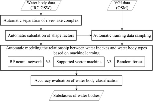
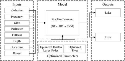
The method shown in Figure 2 consists of five parts: automatic separation of river–lake complexes, automatic calculation of shape indexes, automatic training data sampling, automatic modelling the relationship between water indexes and water body types based on machine learning, and accuracy evaluation of water body classification.

Figure 2. Overview of the method (JRC GSW: Joint Research Centre Global Surface Water; VGI: Volunteered Geographic Information; OSM: Open Street Map).

3.1. Automatic separation of river–lake complexes

River–lake complexes are composed of interconnected rivers and lakes and have the morphological characteristics of both rivers and lakes. River–lake complexes are common in large-scale water objects, affecting the accuracy of water body classification. Dividing river–lake complexes into lakes and rivers is important.

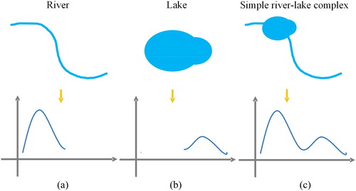
In visual interpretation, river–lake complexes are split according to the obvious differences in the width between the lakes and the rivers. How to determine the differences using a computer is the key of automatic separation of river–lake complexes. Some studies of river morphology showed that the widths of a river collected along the river direction with a certain interval are either skew or normal distribution (Allen and Pavelsky 2015; Allen et al. 2018), as shown in Figure 3(a), where the distribution is a single peak distribution. Similar findings were reported for lakes, as shown in Figure 3(b). Therefore, the width of a simple river–lake complex with only a river and a lake has a bimodal distribution, as shown in Figure 3(c). The bimodal distribution was accepted as a characteristic of a simple river–lake complex in this study.

Figure 3. The width distributions of (a) a river, (b) a lake, and (c) a simple river–lake complex.

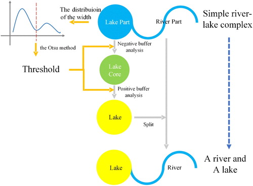
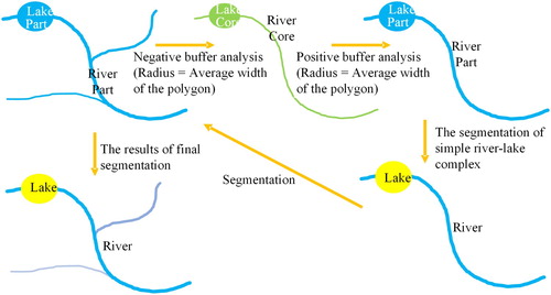
For the separation of a simple river–lake complex, as shown in Figure 4, the segmentation threshold is first determined between the bimodal distribution using the Otsu method (Otsu 1979), and then a negative buffer analysis is conducted with the threshold for the simple river–lake complex to obtain the core of the lake. Finally, a positive buffer analysis is performed with the threshold for the ‘core’ to obtain the lake. Following the three steps, the river and the lake can be separated from the simple river–lake complex.

Figure 4. The separation process of a simple river–lake complex.

If a river–lake complex is not simple, it is called a combined river–lake complex in this paper. A combined river–lake complex contains different sized lakes and rivers. Its width distribution has no typical characteristics from the statistics viewpoint. After careful study, the average width of a river–lake complex was found to be useful for the separation of a combined river–lake complex. Similarly, for the separation processes of a simple river–lake complex using the average width as segmentation threshold, the river–lake complex is divided into several parts, which may include single lakes, single rivers, simple river–lake complexes, and combined river–lake complexes, as shown in Figure 5. The single lakes and single rivers can be judged by the characteristics of the single peak distribution of their width. The simple river–lake complexes can be divided into lakes and rivers by the process as shown in Figure 4. The combined river–lake complexes can be continually processed using the same method.

Figure 5. The separation process of a combined river–lake complex.

We needed to determine how to calculate the widths of rivers and lakes. In this study, the water bodies are vector polygonal data, and the edges of the polygons are connected by a large number of discrete points in turn. As long as the distance between these discrete points and the opposite bank of the river–lake complex is calculated, it is equivalent to the width of the river–lake complex from this point to the opposite bank. To calculate the width without the aid of flow direction, the tangent direction of the discrete point is considered as the direction parallel to the flow direction. Starting from a point, a straight line is drawn perpendicular to the tangent direction of the point. One of the intersections between the river–lake complex and this straight line is the point on the opposite bank. The distance between the two points is calculated, and then the width can be obtained.

Considering the separation idea of a river–lake complex, the method of automatic separation of river–lake complex can be expressed using Algorithm 1.

Table

Algorithm 1. The method of automatic separation of a river–lake complex.

Inputs: I (vector polygonal data of water bodies derived from JRC GSW)

Outputs: O (vector polygonal data of rivers and lakes)

Steps:

1. Read each water polygon (EWP) in the I in turn

2. Calculate the width distribution of EWP

3. Judge the width distribution type of EWP:

3.1 Single peak distribution: The EWP may be a river or a lake, then skip to step 6.

3.2 Bimodal distribution: The EWP is a simple river–lake complex, then skip to step 4.

3.3 Non-single-peak distribution and non-bimodal distribution: The EWP is a combined river–lake complex, then skip to step 5.

4. Split a simple river–lake complex:

4.1 Read the width distribution of the EWP, and use the Otsu method to determine the segmentation threshold (ST).

4.2 Perform negative buffer analysis for the EWP with ST, and then perform positive buffer analysis for the EWP with ST. Therefore, the EWP is split into water polygons (WP) as a river and a lake.

4.3 Delete the EWP from I, and put the WP into O. Skip to step 6.

5. Split a combined river–lake complex:

5.1 Calculate the average width of the EWP, and the average width is taken as the segmentation threshold (ST).

5.2 Conduct negative buffer analysis for the EWP with ST, and then perform positive buffer analysis for the EWP with ST. Therefore, the EWP is split into water polygons (WPs).

5.3 Delete the EWP from I, and put the WP into I. Return to step 1.

6. Judge the number of water polygons in I:

6.1 The number of water polygons in I is 0: Stop the algorithm.

6.2 The number of water polygons in I is not 0: Return to step 1.

3.2. Automatic training data sampling

Sampling water bodies data were used for training the machine learning model. The idea of automatic training data sampling involves transferring the water subclass information to the water polygon in the JRC GSW data. Two steps are followed to sample the training data: judging the water subclass according to the attributes of the water polygon in the OSM data, then labelling the water subclass information to the water polygon in JRC GSW data according to the spatial position relationship between the OSM data and JRC GSW data, and then adopting the labelled JRC GSW data as the training data.

The water subclass is judged according to the attributes of the water polygon in the OSM data. For OSM data, the information recorded by ‘fClass’ and ‘name’ can be used to determine whether the water body is a lake or a river. In ‘fClass’, the label ‘reservoir’ is described as an artificial lake, so the water object with the label ‘reservoir’ can be determined to be a lake; whereas the label ‘River’ is described as a river, so the water objects with the label ‘River’ can be determined to be rivers. The information recorded by ‘name’ is the name of the water object. In Chinese, the names of lakes and rivers have obvious regularity, that is, lakes are generally named ‘XX湖’ and ‘XX池’, and rivers are generally named as ‘XX河’, ‘XX江’ and ‘XX水’. In English, lakes are generally named ‘XX Lake’, and rivers are generally named ‘XX River’. Therefore, the subclass of the water object can be determined according to the last word of water name recorded by ‘name’. After investigation and summary, a mapping table was obtained to determine the subcategory of water objects according to the last word in ‘name’, as shown in Table 2. In this study, we first judged the water object subclass according to the information recorded by ‘fClass’. If the information recorded by ‘fClass’ cannot judge the water object subclass or the information is null, then the water object subclass is judged according to the information recorded by ‘name’.

Table 2. The relationship between the ending word in “name” and the water subclass.

The last word of “name”	The water subclass
“河”, “江”, “川”, “溪”, “渠”, “river”	River
“湖”, “错”, “池”, “塘”, “海”, “水库”, “荡”, “淀”, “lake”	Lake

The water subclass information was labelled to the water polygon in the JRC GSW data according to the spatial position relationship between the OSM and JRC GSW data. According to the spatial position relationship, the corresponding relationship between the polygon of water layer and the polygon of JRC GSW was mapped. This is essentially a problem of judging the spatial relationship between polygons. Judging the spatial position relationship between any two polygons is a time-consuming process. To simplify the calculation, the water polygons in ‘water’ were converted into point features, retaining the ‘fClass’ and ‘name’ data label information. If the transformed point feature of water layer was located in the JRC GSW water polygon, the water subclass information contained in the point feature was transferred to the JRC GSW water polygon. Due to the duplication of OSM data in the collection process, each water object vectored by JRC GSW could have multiple OSM corresponding water objects. If there are multiple OSM water objects corresponding to the water object, the interpretation results of all OSM water objects are counted. If the number of times a certain water subclass appears in the total number of interpretation results is more than 50%, the water object belongs to the water subclass. If the number of times no certain water subclass appears in the total number of interpretation results is more than 50%, the water object subclass is ‘other’.

3.3. Shape factors

To effectively measure the morphological differences of different water objects, we used eight shape factors (cohesion, proximity, girth, perimeter, fullness, depth, dispersion, and range) to measure the morphological characteristics of water objects. These eight shape factors reflect the compactness of shape from different angles. The specific definitions and calculation formulas are provided in Table 3.

Table 3. The definition and calculation formulas of the eight shape factors from the paper (Angel, Parent, and Civco 2010).

Name	Definition	Calculation scheme
cohesion	The Cohesion Index is the ratio of the average distance-squared among all points in an equal-area circle and the average distance-squared among all points in the shape.	$d_{IS}=\left({\displaystyle \frac{1}{n^2}}\right)\cdot \sum _{i=1}^n\sum _{j=1}^n(x_i+x_j{)}^2+(y_i+y_j{)}^2$ $d_{IA}=R_A^2$ $I_c={\displaystyle \frac{d_{IA}}{d_{IS}}}$ $I_C$: cohesion index; $x_i,y_i$: the coordinates of any point in the shape $d_{IS}$: inter-point distance-squared between a sample of n random points in the shape; $\mathrm{n}$: n random points in the shape; $d_{IA}$ the average inter-point distance-squared in a circle of area; $R_A$: the average inter-point distance-squared in a circle of radius.
proximity	The Proximity Index is the ratio of the average distance from all points in the equal-area circle to its centre and the average distance to the Proximate Centre (the centre of gravity of a shape) from all points in the shape.	$d_{CS}=\left({\displaystyle \frac{1}{n^2}}\right)\cdot \sum _{i=1}^n\sum _{j=1}^n(x_i+x_c{)}^2+(y_i+y_c{)}^2$ $d_{CA}={\displaystyle \frac{2R_A}{3}}$ $I_Y={\displaystyle \frac{d_{CA}}{d_{CS}}}$ $I_Y$: proximity index; $x_i,y_i$: the coordinates of any point in the shape; $x_c,y_c$: the coordinates of the Proximate Centre; $d_{CS}$: the average distance to the Proximate Centre of the shape; $R_A$: the radius of the equal-area; $d_{CA}$: The average distance to the centre of the equal-area circle of radius $R_A$.
girth	The Girth Index is the ratio of the thickest layer insulating the innermost point (the point of a shape that is furthest away from its periphery) of the shape from its periphery and the radius of the equal-area circle.	$I_G={\displaystyle \frac{R_s}{R_A}}$ $R_A=\sqrt{{\displaystyle \frac{A}{\pi }}}$ $I_G:$ girth index; $R_s$: the radius of the largest circle circumscribed by the shape; $R_A$: the radius of the equal-area circle; $A:$ the area of the shape.
perimeter	The Perimeter Index is the ratio of the perimeter of the equal-area circle and the perimeter of the shape.	$I_p={\displaystyle \frac{P_A}{P}}$ $I_p$: perimeter index; $P_A:$ the perimeter of the equal-area circle; $P:$ the perimeter of a shape.
fullness	Fullness is the share of the area of a small neighbourhood that belongs to the shape, rather than to its periphery.	$I_F={\displaystyle \frac{F_s}{0.957}}$ $r_A=\sqrt{\left({\displaystyle \frac{A}{100\pi }}\right)}$ $F_s={\displaystyle \frac{{\sum }_{i=1}^m{F}_i}{n}}$ $F_s={\displaystyle \frac{\left({\sum }_{i=1}^n{F}_i\right)}{n}}$ $I_F$: fullness index; $r_A:$ the radius of a small neighbourhood in the shape; $F_i:$ the fullness of a small circle of radius $r_A$; $F_s$: the average fullness of the fullness $F_i$.
depth	The Depth Index is the ratio of the average distance to the periphery in the shape and the average distance to the periphery in its equal-area circle.	$I_H={\displaystyle \frac{d_{PS}}{d_{PA}}}$ $d_{PA}={\displaystyle \frac{R_A}{3}}$ $I_H$: depth index; $d_{PS}:$ the average straight-line distance from the centres of all pixels to the outer periphery of the shape; $d_{PA}$: the average distance to the periphery of the equal-area circle.
dispersion	The dispersion index of a given shape is the ratio of the area of the shape inside the Average-Distance circle (a circle about the centre of a given shape with a radius equal to the average distance of points on the perimeter of the shape to its centre) and the area of the Average-Distance Circle.	$I_D={\displaystyle \frac{A-A_o}{A}}$ $I_D$: dispersion index; $A_o:$ the area of a shape outside the Average Distance Circle; .
range	The Range Index of a given shape is the ratio of the diameter of its equal-area circle and the diameter of the smallest circle fully circumscribing the shape.	$I_R=D_A/D_s$ $I_R:$ range index $D_A$: the diameter of the equal-area circle; $D_s$: the diameter of the smallest circle circumscribing the given shape.

3.4. Automatic modelling the relationship between water shape factors and water body types based on machine learning

We separated the rivers and lakes using their different morphological characteristics. We modelled the relationship between water factors and water body types based on machine learning. A single shape factor cannot fully reflect the difference between lakes and rivers. In this study, eight shape factors were used as model inputs, and the output of the model was lakes and rivers. Due to the lack of literature on the application of machine learning to model the relationship between water factors and water body types, we explored the applicability of three common machine learning models: back propagation (BP) neural network, random forest (RF), and support vector machine (SVM). The method is shown in Figure 6.

Figure 6. The method of modelling the relationship between water factors and water body types based on machine learning.

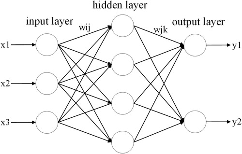
3.4.1. BP neural network

BP neural network is a method based on the error back propagation algorithm to minimize the total output error (or average error) of the network in the training process (Hornic 1989). Figure 7 shows an example of such a network. In the network, there is an input layer, an output layer, and one or more hidden layers.

Figure 7. An example of a back propagation (BP) neural network.

Taking a network with n inputs, m outputs and s hidden layer nodes for example, the total output error e is the sum of the difference between every output of the network $y_k$ and its desired output $t_k$ which is provided by samples, hence the error formula is:(1) $\begin{array}{c}e=\sum _{k=1}^m{\left(t_k-y_k\right)}^2.\end{array}$(1)

Every output $y_k$ is equal to:(2) $\begin{array}{c}{y}_k=\varphi \left(\sum _{j=1}^s{w}_{jk}{b}_j-{\theta }_k\right)\left(j=1,2,\dots ,s;k=1,2,\dots m\right).\end{array}$(2) $\varphi$ is the activation function in the output layer, $w_{jk}$ is the weight between hidden layer and output layer, $h_j$ is the output of every hidden layer node calculating from the input layer, and ${\theta }_k$ is the bias of every hidden layer node.

The formula of $h_j$ is defined as:(3) $\begin{array}{c}{h}_j=\tau \left(\sum _{i=1}^n{w}_{ij}{x}_i-{\theta }_j\right)\left(\mathrm{i}=1,2,\dots ,\mathrm{n};\mathrm{j}=1,2,3,\dots ,\mathrm{s}\right).\end{array}$(3) $\tau$ is the activation function in the hidden layer, $w_{ij}$ is the weight between the input layer and the hidden layer, $x_i$ is the input of the network that is provided by the samples.

Every training process of the network is calculating the total output error e according to the formula (1), (2), (3) and using the error back propagation algorithm to adjust the weight and bias in the network to make e as small as possible. And repeat the training process constantly until the minimum e can be obtained.

3.4.2. Support vector machine

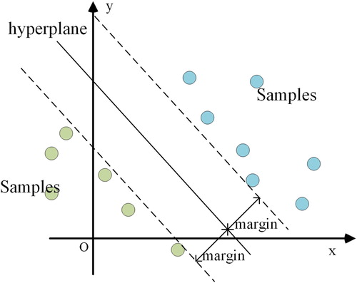
Support vector machine (SVM) is a commonly used machine learning model for binary classification problems. According to a certain transformation function, the model maps the training samples to a high-dimensional space and searches for the hyperplane which makes the distance between the two types of training samples the largest, and this hyperplane is the classification standard of the experimental data (Talukdar et al. 2020). An example of SVM is illustrated in Figure 8.

Figure 8. An example of a support vector machine (SVM).

The hyperplane is defined in n-dimensional space as:(4) $\begin{array}{c}{\omega }^{T}x+b=0\end{array}$(4)

The distance d from vector of the sample to the hyperplane, that is, the distance between the point and the hyperplane in n-dimensional space is:(5) $\begin{array}{c}d=\frac{\left|{\omega }^{T}x+b\right|}{\omega }\end{array}$(5)

To maximize the d, formula (5) can be further simplified as:(6) $\begin{array}{c}d=\mathrm{m}\mathrm{a}\mathrm{x}\frac{2}{\omega }\end{array}$(6)

Maximizing the d is equivalent to minimizing the its inverse, hence the optimization of d is equivalent to solving the minimum value of the above formula (6):(7) $\begin{array}{c}\underset{w,b}{min}y\frac{1}{2}{\omega }^2\\ s.t.y_i\left({\omega }^T{x}_i+b\right)\ge 1,i=1,\end{array}$(7)

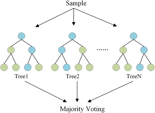
3.4.3. Random forest

Random forest (RF) is an ensemble classification algorithm (Talukdar et al. 2020), as shown in Figure 9, which uses decision tree as the basic classifier. For input vector (classified eigenvector) X and output vector (classified result) Y, the training process of random forest is to find a prediction function to simulate the relationship between X and Y. The accuracy of the prediction function is determined by the loss function:(8) $\begin{array}{c}L\left(Y,f\left(X\right)\right)=I\left(Y\ne f\left(X\right)\right)=\left\{\begin{array}{c}0\mathrm{i}\mathrm{f}Y=f\left(x\right)\\ 1\mathrm{o}\mathrm{t}\mathrm{h}\mathrm{e}\mathrm{r}\mathrm{w}\mathrm{i}\mathrm{s}\mathrm{e}\end{array}\right.\end{array}$(8)

Figure 9. An example of random forest (RF).

When the mathematical expectation of loss function $E_{XY}\left(L\left(Y,f\left(X\right)\right)\right)$ is the lowest, prediction function $f\left(X\right)$ that can simulate the relationship between X and Y. The minimum value of $E_{XY}\left(L\left(Y,f\left(X\right)\right)\right)$ can be expressed as:(9) $\begin{array}{c}f\left(x\right)=\mathrm{a}\mathrm{r}\mathrm{g}\mathrm{m}\mathrm{a}\mathrm{x}P\left(Y=y|X=x\right)\left(y\in Y\right)\end{array}$(9)

Random forest integrates a set of basic learners, that is, decision trees can be further expressed as:(10) $\begin{array}{c}f\left(x\right)=\mathrm{a}\mathrm{r}\mathrm{g}\mathrm{m}\mathrm{a}\mathrm{x}\sum _{j=1}^{J}I\left(y=h_j\left(x\right)\right)\left(y\in Y\right)\end{array}$(10)

The basic learner can be further represented as $h_j\left(X,{\mathrm{\Theta }}_j\right)$, in which ${\mathrm{\Theta }}_j$ is randomly selected variables from the input vector.

3.5. Accuracy evaluation of water body classification

Accuracy evaluation was used to quantify the accuracy of the proposed automatic water classification method. Because there were no corresponding real distribution data of lakes and rivers, in this study, visual interpretation was used to verify the largest surface water products for each year. For each year's classification results, 500 water objects were randomly selected. Then, through visual interpretation, we judged whether these water objects were lakes or rivers. Finally, the classification accuracy was calculated by comparing the results of visual interpretation with the experimental classification results. The accuracy calculation formula is as follows:(11) $\begin{array}{c}\mathrm{A}\mathrm{c}\mathrm{c}\mathrm{u}\mathrm{r}\mathrm{a}\mathrm{c}\mathrm{y}=\frac{\mathrm{C}\mathrm{o}\mathrm{r}\mathrm{r}\mathrm{e}\mathrm{c}\mathrm{t}}{\mathrm{S}\mathrm{a}\mathrm{m}\mathrm{p}\mathrm{l}\mathrm{e}\mathrm{s}}\end{array}$(11) where Accuracy is the accuracy, Correct is the correct classification number, and Samples is the total number of samples for visual interpretation.

In addition, the kappa coefficient, a common measurement accuracy index used for classification problems, was adopted in this study. The kappa coefficient is calculated as follows:(12) $\begin{array}{c}\mathrm{K}\mathrm{a}\mathrm{p}\mathrm{p}\mathrm{a}=\frac{\mathrm{A}\mathrm{c}\mathrm{c}\mathrm{u}\mathrm{r}\mathrm{a}\mathrm{c}\mathrm{y}-D}{1-D}\end{array}$(12) (13) $\begin{array}{c}D=\frac{a_1\times b_1+a_2\times b_2+\dots +a_n\times b_n}{\mathrm{S}\mathrm{a}\mathrm{m}\mathrm{p}\mathrm{l}\mathrm{e}\mathrm{s}\times \mathrm{S}\mathrm{a}\mathrm{m}\mathrm{p}\mathrm{l}\mathrm{e}\mathrm{s}}\end{array}$(13) where Kappa is the kappa coefficient, D is the calculation intermediate quantity, a_n is the number of visual interpretation for each category, and b_n is the number of experimental categories.

4. Results

4.1. Separation of river–lake complexes

According to the method proposed in Section 3.1, JRC GSW data in the Yangtze River basin from 2008 to 2018 were split. Table 4 shows the number of water objects in the basin before and after the separation of the river–lake complexes in different years. In terms of quantity, the impact of river–lake complexes is between 3008 and 4697. In terms of percentage, the impact of river–lake complexes is between 3.56% and 5.70%.

Table 4. the number of water objects in the basin before (B) and after (A) the separation of the river–lake complexes in different year, as well as the changes (C = (A–B)/B ×100).

	2008	2009	2010	2011	2012	2013	2014	2015	2016	2017	2018
B	68181	71042	65676	63274	59018	70077	72563	66581	85187	85640	90685
A	71652	74460	69094	66282	61886	73509	76531	70373	88217	90125	95382
A-B	3471	3418	3418	3008	2868	3432	3968	3792	3030	4485	4697
C(%)	5.09	4.81	5.20	4.75	4.86	4.90	5.47	5.70	3.56	5.24	5.18

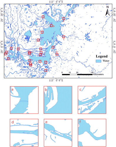
To visualize the results of the separation, three big lakes (Chaohu Lake, Poyang Lake, and Dongting Lake) were selected as examples to illustrate some details of the results. Figures 10–12 show the results for Chaohu Lake, Poyang Lake, and Dongting Lake, respectively. In Figures 10–12, each red box locates the intersection of a river and a lake; the blue line marks the dividing of the intersection. From visual judgment, the results are reasonable.

Figure 10. The separation results of Chaohu Lake: (a)-(g) the intersection of the river and the lake.

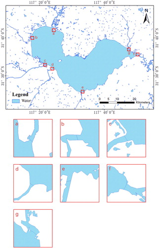
Figure 11. The separation results of Poyang Lake (a)-(f) the intersection of the river and the lake.

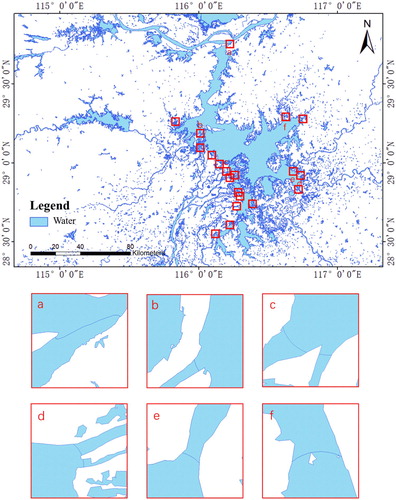
Figure 12. The separation results of Dongting Lake (a)-(f) the intersection of the river and the lake.

4.2. Training data sampling

With the proposed method in Section 3.2, 2034 lake samples and 1116 river samples were collected based on the OSM data and JRC GSW dataset. The smallest area of these samples was 0.030025 km², which means that the morphological characteristics of water objects whose area was smaller than the sample were not collected. This mean the machine learning model was not unable to distinguish the lakes and rivers whose area was smaller than the sample. To ensure the experimental accuracy of automatic classification of lakes and rivers in the Yangtze River basin, we only classified water objects with an area of more than 0.03 km².

4.3. Classification results of lakes and rivers

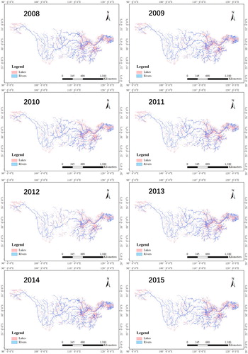
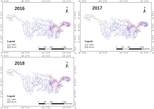
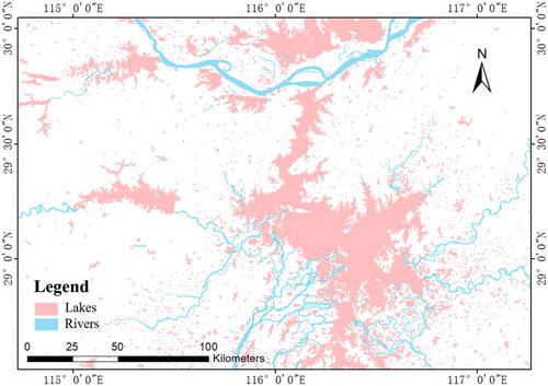
Based on the methods proposed in Section 3.1–3.4, the classification results of rivers and lakes in the Yangtze River basin from 2008 to 2018 were obtained, as shown in Figure 13. Figure 13 shows that the whole Yangtze River and its tributaries were clearly observed and large lakes were extracted.

Figure 13. The classification results of rivers and lakes in the Yangtze River basin from 2008 to 2018.

To more clearly observe the results of water body classification, the water body classification results for Dongting Lake, Wuhan area, and Poyang Lake in 2018 are shown in Figures 14–16. Figure 14 shows that a large number of lakes was extracted and Dongting Lake was successfully separated from the Yangtze River and the rivers flowing into the lake. In the left half of Figure 14, a number of rivers are wrongly divided into lakes, the reasons for which are explained in detail in Section 6.3.5. As shown in Figure 15, the lakes and rivers in the Wuhan area were successfully separated. The Yangtze River passes through the dense lakes in the Wuhan area and divides the whole area into the north and the south. In the area, most of the tributaries of the Yangtze River flow into the Yangtze River from the north bank, and most of the lakes are distributed very close to both sides of the Yangtze River. According to Figure 16, the water body classification effect in the Poyang Lake area was good. Poyang Lake, the Yangtze River and the rivers flowing into Poyang Lake form a lake–river waterbody complex, which was successfully split. We found that all parts of the complex were divided into the correct water body subclasses. The reservoir on the left side of Figure 16 and the rivers connected with it form a water body complex of lakes and rivers, and each part of the complex after separation was classified into the correct water body subclass. Observing the distribution of lakes and rivers in Figure 16, we found that the distribution of lakes in the Poyang Lake area is centred on Poyang Lake, and the closer to the Poyang Lake area, the denser the distribution of lakes.

Figure 14. Classification results of Dongting Lake in 2018.

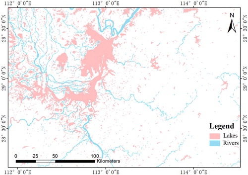
Figure 15. Classification results of the Wuhan area in 2018.

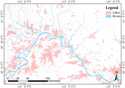
Figure 16. Classification results of Poyang Lake in 2018.

Based on the classification results, the number and area of lake objects in 2008–2018 were counted, as shown in Tables 5 and 6, respectively. Their corresponding line graphs are shown in Figures 17 and 18, respectively.

Figure 17. The number of lakes from 2008 to 2018.

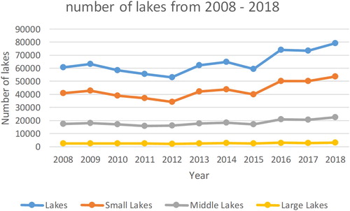
Figure 18. The areas of the lakes from 2008 to 2018.

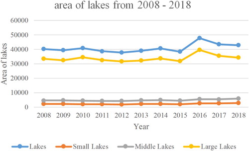
Table 5. The numbers of lakes from 2008 to 2018. AL: all lakes, SL: small Lakes, ML: medium lakes, LL: large lakes.

	2008	2009	2010	2011	2012	2013	2014	2015	2016	2017	2018
AL	60722	63311	58518	55483	53170	62276	64761	59486	73893	73483	79020
SL	40865	42769	39073	37226	34248	42062	43805	40123	50060	50077	53707
ML	17418	18037	16945	15915	16204	17695	18329	16943	20944	20705	22386
LL	2439	2505	2500	2342	2218	2519	2627	2420	2889	2701	2927

Table 6. The areas of the lakes from 2008 to 2018 (Unit: km²). AL: All lakes, SL: Small Lakes, ML: Medium lakes, LL: Large lakes.

	2008	2009	2010	2011	2012	2013	2014	2015	2016	2017	2018
AL	40231	39370	40791	38690	37693	39004	40708	38290	47712	43484	42925
SL	2124	2225	2032	1939	1821	2189	2273	2081	2606	2606	2797
ML	4556	4722	4521	4207	4290	4587	4799	4421	5461	5363	5845
LL	33549	32422	34417	32543	31581	32228	33635	31786	39644	35515	34281

Through statistical analysis of the classification results from 2008 to 2018, the number of lakes showed an upward trend, and the total area of lakes basically remained unchanged. In these 11 years, 2018 had the largest number of lakes, with 79,020, and 2011 had the smallest number of lakes, with 55,483; 2016 had the largest lake area, at 47,712 km², and 2012 had the smallest lake area, at 37,693 km². The changes in the number and area of small, medium, and large lakes were similar to that of all lakes. In the 11 years, 2018 had the largest numbers of small, medium, and large lakes, with 53,707, 22,386, and 2927, respectively; 2012 had the smallest numbers of small and large lakes, with 34,248 and 2218, respectively; 2011 had the smallest number of medium lakes, with 15,915. In 2018, the area of small- and medium-sized lakes was the largest, at 2797 and 5845 km², respectively. In 2016, the area of the large lakes was the largest, at 39,644 km². The smallest area of small and large lakes occurred in 2012, at 1821 and 31581 km², respectively; 2011 had the smallest medium lake area, at 4207 km². The small lakes dominated in the number of lakes and the area of large lakes dominated the area of lakes in the Yangtze River basin.

4.4. Accuracy evaluation

4.4.1. Optimal parameter evaluation of machine learning method

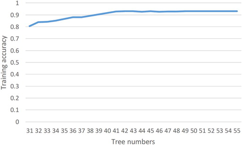
The parameter optimization of the BP neural network and RF is important for improving the accuracy of classification results. Although many studies introduced calculation formulas for the best number of nodes for BP neural networks and the best number of trees for RF, the results of the calculation formulas are different. Therefore, the best number of nodes and the best number of trees can be determined through repeated experiments. Figure 19 shows the different accuracy of different nodes of a BP neural network. Figure 20 shows the different accuracy corresponding to different RF tree numbers. Figure 19 shows that the change in the BP neural network using 20 nodes was not large, so 20 was selected as the node number for the BP neural network. For the RF in Figure 20, the training accuracy changed little after 50, so the number of trees in the random forest was set to 50.

Figure 19. BP neural network training accuracy with different numbers of hidden layer nodes.

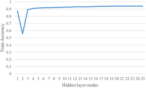
Figure 20. RF training accuracy with different numbers of trees.

4.4.2. Accuracy evaluation of classification results

The accuracy and kappa coefficient of the experimental classification results under three machine learning models (BP neural network, SVM, and RF) are shown in Table 7, and the corresponding line chart is provided in Figure 21. From Table 7 and Figure 21, the classification accuracy of BP method was between 90% and 94% and the kappa was above 0.65 in 2008–2018; the classification accuracy of RF method was between 90% and 94% and the kappa was above 0.6 in 2008–2018; the classification accuracy of SVM was between 90% and 92% and the kappa was above 0.6 in 2008–2018. Therefore, the method can distinguish lake and river targets correctly, and the performance is stable. The accuracies of the three machine learning classification results were similar, and the accuracy difference between different machine learning models was within 3%. Although the accuracy of SVM was significantly lower than the other two machine learning models in 2015, the difference between the accuracy values was still within 3%.

Figure 21. The accuracy of the classification results under BP, RF, and SVM from 2008 to 2018.

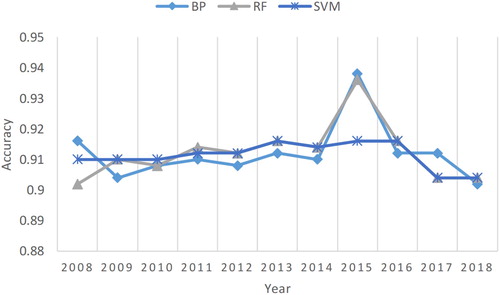
Table 7. The accuracy and kappa coefficient of classification results under BP, RF, and SVM from 2008 to 2018.

Year	BP		RF		SVM
	Accuracy	Kappa	Accuracy	Kappa	Accuracy	Kappa
2008	0.916	0.71345	0.902	0.66983	0.91	0.68644
2009	0.904	0.69589	0.91	0.70743	0.91	0.69839
2010	0.908	0.6544	0.908	0.61377	0.91	0.60106
2011	0.91	0.728	0.914	0.7347	0.912	0.73131
2012	0.908	0.65824	0.912	0.67623	0.912	0.67623
2013	0.912	0.69589	0.916	0.68773	0.916	0.68773
2014	0.91	0.71994	0.914	0.71814	0.914	0.71814
2015	0.938	0.80253	0.936	0.77824	0.916	0.72063
2016	0.912	0.72113	0.916	0.72983	0.916	0.65255
2017	0.912	0.73672	0.904	0.68304	0.904	0.70487
2018	0.902	0.69976	0.904	0.68992	0.904	0.68992

5. Discussions

5.1. Comparison with related work and advantages

Many previous studies mainly extract water bodies from remote sensing images by water index method (Feyisa et al. 2014; Fisher, Flood, and Danaher 2016; Huang et al. 2018; Khandelwal et al. 2017; Qiao, Zhu, and Yang 2019). The index method only can divide the identified objects into two categories as water body and non-water body. In this paper, the water bodies were further divided into subclass as lakes and rivers. Previous work (Wang, Sheng, and Tong 2014; Yao et al. 2019; Xie et al. 2017; Zhang et al. 2019) about lake extraction from remotely sensed data always including three steps: (1) defining regions of interest (ROIs) for lakes, (2) extracting lakes by water index method, and (3) doing human-interactive quality control. The processes need manual participation and are not high efficient. A full-automatic classification method of water sub classes was proposed without the guidance of ROIs. The proposed method has relatively high efficiency and high accuracy. For long-term and large-scale data, the method proposed in this paper has advantages.

5.2. Error analysis and disadvantages

5.2.1. Fragmented river

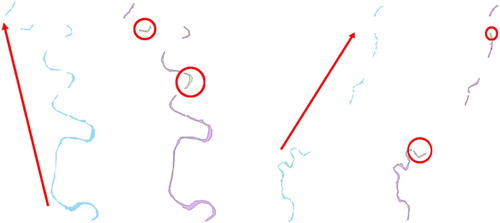
The JRC GSW images used in the experiment were incomplete and fragmented in the extraction results of small water bodies, especially small rivers. Fragmented rivers were easily misclassified, as shown in Figure 22. The rivers, which should be characterized by lengths far greater than widths, became water objects with discrete surface elements similar to lakes whose length and width are similar. Therefore, this river debris was easily mistakenly classified as lake. The method proposed in this paper does not handle the incomplete and fragmented water bodies before classification. The key aspect of the difficulty is that limited contextual information is available to handle the problem. A DEM-based product, e.g. the SRTM Water Body Dataset (accessed at https://lpdaac.usgs.gov), may help solve the river continuity problem. Future work will focus on improving the proposed method in the paper with a DEM-based product.

Figure 22. Incomplete and fragmented extraction of JRC GSW small water bodies producing errors.

5.2.2. Unchecked training samples

The OSM data used in this paper were unchecked. The lake and river information recorded by OSM may not be correct, resulting in the incorrect marking of training samples. When volunteers collect OSM data, due to subjective or objective reasons, the uploaded data may differ from the actual situation. If training samples contain wrong data, the accuracy of the final water classification would be affected. Future work will focus on the correction of OSM sampling data.

5.2.3. Overlapped shape factors

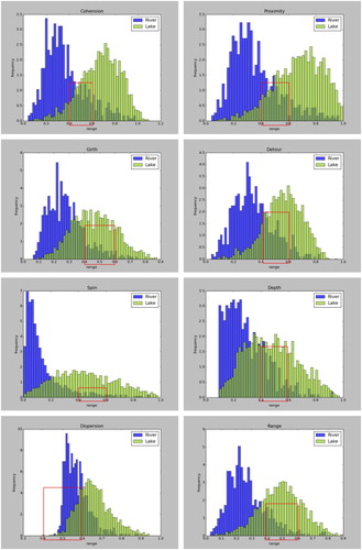
Each shape factor is proposed for specific morphological characteristics; each shape factor can only quantitatively describe one aspect of the shape of a water body. Although we used eight shape factors to distinguish lakes and rivers, the shape factors had some common overlapping results. As shown in Figure 23, we calculated the frequency distributions of rivers and lakes in different ranges of each shape factor. In the range of 0.4–0.6, the frequency distributions of the eight shape factors overlap. This leads to the occurrence of misclassifications. In addition, the shape factor requires a water body to have a certain size. When the size is too small, the shape factor cannot effectively reflect its morphological characteristics. This limits the ability of the shape factor to distinguish small lakes and rivers. Further work will focus on adding other but non-shape features as the inputs of the machine learning method.

Figure 23. The frequency distributions of rivers and lakes in different ranges for each of the eight shape factors: (a) cohesion, (b) proximity, (c) girth, (d) perimeter, (e) fullness, (f) depth, (g) dispersion, and (h) range.

6. Conclusions and future work

Calculating long-term and large-scale lake statistics is labour-intensive and time-consuming. This paper proposed a novel method for lake extraction via water body classification. The method includes three aspects: separation of river–lake complexes, training data sampling, and shape-factors- and machine-learning-based water body classification. The method was constructed by programming. Taking the Yangtze River Basin as the study area and based on JRC GSW and OSM data, we extracted lakes from 2008 to 2018. The main conclusions are as follows:

• A method for separation of river–lake complexes based on the width distribution was proposed in this paper. The river–lake complexes from 2008 to 2018 in the Yangtze River basin were successfully separated. In terms of quantity, the river–lake complexes number between 3008 and 4697. In terms of percentage, the river lake complexes account for between 3.56% and 5.70%.

• A method for long-term and large-scale lake extraction based on shape factors and machine learning by water body classification was proposed in this paper. The water bodies in the Yangtze River basin from 2008 to 2018 were classified as shown in Figure 13. The number and the area of the lakes and rivers in the Yangtze River Basin were determines (Tables 5 and 6). The accuracy of water classification in each year was stable between 90.2% and 93.6%. In comparing the BP, RF, and SVM machine learning models, we found that they have similar classification accuracies in this scenario.

• Fragmented and incomplete small rivers in the JRC GSW data, unchecked training samples, and overlapping shape factors are the three error sources of the proposed method.

To handle the three error sources of the proposed method, future work will focus on a method of judging the same object with multiple water bodies, the correction of OSM data, and using other types of inputs other than shape factors to distinguish water bodies.

Disclosure statement

No potential conflict of interest was reported by the author(s).

Data Availability Statement

The JRC GSW dataset is referenced by the paper (Pekel et al. 2016). The openstreetmap data is referenced by the website (https://www.openstreetmap.org). The results of this paper can be asked by corresponding email.

Additional information

Funding

This work was supported by the National Nature Science Foundation of China (nos. 41971351, 41771422, 41890822).

References

- Allen, G. H., and T. M. Pavelsky. 2015. “Patterns of River Width and Surface Area Revealed by the Satellite-Derived North American River Width Data set.” Geophysical Research Letters 42 (2): 395–402. doi:10.1002/2014GL062764.
- Allen, G. H., T. M. Pavelsky, E. A. Barefoot, M. P. Lamb, D. Butman, A. Tashie, and C. J. Gleason. 2018. “Similarity of Stream Width Distributions Across Headwater Systems.” Nature Communications 9 (1): 610. doi:10.1038/s41467-018-02991-w.
- Angel, S., J. Parent, and D. L. Civco. 2010. “Ten Compactness Properties of Circles: Measuring Shape in Geography.” The Canadian Geographer 54 (4): 441–461. doi:10.1111/j.1541-0064.2009.00304.x.
- Ballatore, A., M. Bertolotto, and D. C. Wilson. 2013. “Geographic Knowledge Extraction and Semantic Similarity in OpenStreetMap.” Knowledge and Information Systems 37 (1): 61–81. doi:10.1007/s10115-012-0571-0.
- Chen, J., J. Chen, A. Liao, X. Cao, L. Chen, X. Chen, C. He, et al. 2015. “Global Land Cover Mapping at 30 m Resolution: A POK-Based Operational Approach.” ISPRS Journal of Photogrammetry and Remote Sensing 103: 7–27. doi:10.1016/j.isprsjprs.2014.09.002.
- Downing, J. A., J. J. Cole, C. A. Duarte, J. J. Middelburg, J. M. Melack, Y. T. Prairie, P. Kortelainen, R. G. Striegl, W. H. Mcdowell, and L. J. Tranvik. 2012. “Global Abundance and Size Distribution of Streams and Rivers.” Inland Waters 2 (4): 229–236. doi:10.5268/IW-2.4.502.
- Feyisa, G. L., H. Meilby, R. Fensholt, and S. R. Proud. 2014. “Automated Water Extraction Index: A new Technique for Surface Water Mapping Using Landsat Imagery.” Remote Sensing of Environment 140: 23–35. doi:10.1016/j.rse.2013.08.029.
- Fisher, A., N. Flood, and T. Danaher. 2016. “Comparing Landsat Water Index Methods for Automated Water Classification in Eastern Australia.” Remote Sensing of Environment 175: 167–182. doi:10.1016/j.rse.2015.12.055.
- Goodchild, M. F. 2007. “Citizens as Sensors: The World of Volunteered Geography.” GeoJournal 69 (4): 211–221. doi:10.1002/9780470979587.ch48 doi: 10.1007/s10708-007-9111-y
- Guo, H., Q. Hu, Q. Zhang, and S. Feng. 2012. “Effects of the Three Gorges dam on Yangtze River Flow and River Interaction with Poyang Lake, China: 2003–2008.” Journal of Hydrology 416: 19–27. doi:10.1016/j.jhydrol.2011.11.027.
- Hornic, K. 1989. “Multilayer Feedforward Networks are Universal Approximators.” Neural Networks 2 (5): 359–366. doi:10.1016/0893-6080(89)90020-8.
- Huang, W., B. DeVries, C. Huang, M. W. Lang, J. W. Jones, I. F. Creed, and M. L. Carroll. 2018. “Automated Extraction of Surface Water Extent From Sentinel-1 Data.” Remote Sensing 10 (5): 797. doi:10.3390/rs10050797.
- Jiang, T., B. Su, and H. Hartmann. 2007. “Temporal and Spatial Trends of Precipitation and River Flow in the Yangtze River Basin, 1961–2000.” Geomorphology 85 (3-4): 143–154. doi:10.1016/j.geomorph.2006.03.015.
- Jiao, L., Y. Liu, and H. Li. 2012. “Characterizing Land-use Classes in Remote Sensing Imagery by Shape Metrics.” ISPRS Journal of Photogrammetry and Remote Sensing 72: 46–55. doi:10.1016/j.isprsjprs.2012.05.012.
- Khandelwal, A., A. Karpatne, M. E. Marlier, J. Kim, D. P. Lettenmaier, and V. Kumar. 2017. “An Approach for Global Monitoring of Surface Water Extent Variations in Reservoirs Using MODIS Data.” Remote Sensing of Environment 202: 113–128. doi:10.1016/j.rse.2017.05.039.
- Lehner, B., and P. Döll. 2004. “Development and Validation of a Global Database of Lakes, Reservoirs and Wetlands.” Journal of Hydrology 296 (1-4): 1–22. doi:10.1016/j.jhydrol.2004.03.028.
- Ma, Y., H. Wu, L. Wang, B. Huang, R. Ranjan, A. Zomaya, and W. Jie. 2015. “Remote Sensing Big Data Computing: Challenges and Opportunities.” Future Generation Computer Systems 51: 47–60. doi:10.1016/j.future.2014.10.029.
- Neis, P., D. Zielstra, and A. Zipf. 2012. “The Street Network Evolution of Crowdsourced Maps: OpenStreetMap in Germany 2007–2011.” Future Internet 4 (1): 1–21. doi:10.3390/fi4010001.
- Otsu, N. 1979. “A Threshold Selection Method From Gray-Level Histograms.” IEEE Transactions on Systems Man & Cybernetics 9 (1): 62–66. doi:10.1109/TSMC.1979.4310076.
- Pekel, J. F., A. Cottam, N. Gorelick, and A. S. Belward. 2016. “High-resolution Mapping of Global Surface Water and its Long-Term Changes.” Nature 540 (7633): 418–422. doi:10.1038/nature20584.
- Qiao, B., L. Zhu, and R. Yang. 2019. “Temporal-spatial Differences in Lake Water Storage Changes and Their Links to Climate Change Throughout the Tibetan Plateau.” Remote Sensing of Environment 222: 232–243. doi:10.1016/j.rse.2018.12.037.
- Rana, S., and T. Joliveau. 2009. “NeoGeography: An Extension of Mainstream Geography for Everyone Made by Everyone.” Journal of Location Based Services 3 (2): 75–81. doi:10.1080/17489720903146824.
- Talukdar, S., P. Singha, S. Mahato, Shahfahad, S. Pal, Y. Liou, and A. Rahman. 2020. “Land-Use Land-Cover Classification by Machine Learning Classifiers for Satellite Observations—A Review.” Remote Sensing 12 (7): 1135. doi:10.3390/rs12071135.
- van der Werff, H. M. A., and F. D. van der Meer. 2008. “Shape-Based Classification of Spectrally Identical Objects.” ISPRS Journal of Photogrammetry and Remote Sensing 63 (2): 251–258. doi:10.1016/j.isprsjprs.2007.09.007.
- Wang, J., Y. Sheng, and T. S. Tong. 2014. “Monitoring Decadal Lake Dynamics Across the Yangtze Basin Downstream of Three Gorges Dam.” Remote Sensing of Environment 152: 251–269. doi:10.1016/j.rse.2014.06.004.
- Xie, C., X. Huang, H. Mu, and W. Yin. 2017. “Impacts of Land-use Changes on the Lakes Across the Yangtze Floodplain in China.” Environmental Science & Technology 51 (7): 3669–3677. doi:10.1021/acs.est.6b04260.
- Yao, F., J. Wang, C. Wang, and J. F. Crétaux. 2019. “Constructing Long-Term High-Frequency Time Series of Global Lake and Reservoir Areas Using Landsat Imagery.” Remote Sensing of Environment 232: 111210. doi:10.1016/j.rse.2019.111210.
- Zhang, G., T. Yao, W. Chen, G. Zheng, C. K. Shum, K. Yang, S. Piao, et al. 2019. “Regional Differences of Lake Evolution Across China During 1960s–2015 and its Natural and Anthropogenic Causes.” Remote Sensing of Environment 221: 386–404. doi:10.1016/j.rse.2018.11.038.