Interactive data styling and multifocal visualization for a multigrid web-based Digital Earth

ABSTRACT

Globe-based Digital Earth (DE) is a promising system that uses 3D models of the Earth for integration, organization, processing, and visualization of vast multiscale geospatial datasets. The growing size and scale of geospatial datasets present significant obstacles to interactive viewing and meaningful visualizations of these DE systems. To address these challenges, we present a novel web-based multiresolution DE system using a hierarchical discretization of the globe on both server and client sides. The presented web-based system makes use of a novel data encoding technique for rendering large multiscale geospatial datasets, with the additional capability of displaying multiple simultaneous viewpoints. Only the data needed for the current views and scales are encoded and processed. We leverage the power of GPU acceleration on the client-side to perform real-time data rendering and dynamic styling. Efficient rendering of multiple views allows us to support multilevel focus+context visualization, an effective approach to navigate through large multiscale global datasets. The client–server interaction as well as the data encoding, rendering, styling, and visualization techniques utilized by our presented system contribute toward making DE more accessible and informative.

KEYWORDS:

• Digital Earth
• Discrete Global Grid System
• data integration
• data fusion
• multilevel focus+context visualization
• spatial resolution
• context awareness

1. Introduction

A globe-based Digital Earth (DE) is a 3D representation of the Earth on which geospatial datasets of multiple different types and scales can be efficiently integrated and visualized using the globe as a reference model (Goodchild 2000). In this approach, a curved Earth is used to model, organize, and visualize geospatial datasets as opposed to 2D map layers used in conventional GIS. Such representations aim to address grand challenges of geosciences – data integration, meaningful visualization, and effective user-interactions (Gil et al. 2018; Liu et al. 2020). It is an important challenge to make large dynamic multiscale datasets accessible, both in terms of their availability and in terms of interactive viewing. Although image-wrapping DE systems such as Google Earth (Google 2020) has made a noticeable impact in the user community through many fascinating applications, they organize geospatial datasets using 2D map layers, and consequently inherit map distortions and positional uncertainty (Goodchild 2018). Alternatively, a multiresolution globe-based DE such as a Discrete Global Grid System (DGGS) can reduce map distortions while supporting multiple resolutions to capture an equal-area sampling of geospatial datasets (Alderson, Mahdavi-Amiri, and Samavati 2016; Alderson et al. 2020; Mahdavi-Amiri, Alderson, and Samavati 2015, 2019). In this work, we detail approaches to tackle the problem of accessing and displaying multiple large datasets in multiple scales at once using a globe-based multiresolution DE. To this end, we introduce a generalized web-based system that supports a novel rendering and visualization framework capable of displaying large multiscale datasets for the entire globe, while allowing for context-aware user-interactions.

To develop this globe-based DE, we face several challenges. The first challenge lies in the size and variety of datasets. A single operation, such as the rendering of the globe, may require the use of several large datasets at varying resolutions. Execution of the underlying queries and rendering of resulting visualizations should be performed in real-time and through interactive interfaces. Another challenge, related to the visualization, is the limitation of screen space, which introduces difficulties in the effective presentation of large differences in scale, large distances between locations on the globe, and the wide varieties of data available. An important challenge is that of visualizing two distant cities, for example, at a detail level high enough to discern roads with a single point of view. Furthermore, datasets often have interesting information at multiple levels of detail. Viewing a dataset at city-scale and country-scale simultaneously is often impossible without special visualization techniques. Likewise, there is a limit to the amount of data that can be overlaid on a single view of the globe.

Finally, the simultaneous integration and visualization of multiple datasets poses another challenge. It becomes even more complicated when combining disparate datasets, such as elevation, cities, roads, labels and population density.

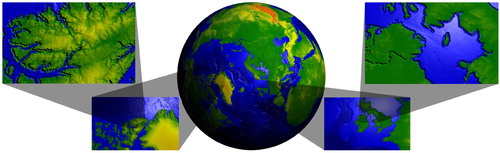
We overcome visualization challenges through the use of multilevel focus+context visualization. We use multiple views of the globe to allow for per-focus styling and scale. In a web-based application, utilizing all required datasets at their native resolution over the entire globe is an extremely slow and resource-intensive approach. Hence, we utilize only what is necessary to accommodate the various views of the globe. For a set of different views, chosen interactively, our system requests only those data required by these views, and at resolutions proportional to the size of the viewports. In summary, our system generates a multi-view aware DE where multiple active views of the globe are concurrently displayed, at a variety of locations and at separate levels of detail, as shown in Figure 1. See Section 6.2 for further related use cases supported by our view-aware DE.

Figure 1. Multilevel focus+context visualization of a DE.

To create an efficient web-based DE framework, we divide the required operations between the server and the web browser application (client). An efficient data structure is required to handle the thousands of pieces of data at multiple resolutions, and geometry of the Earth. This data structure should also facilitate communication between the server and clients. For this purpose, we introduce a new web-based DGGS (Alderson et al. 2020; Mahdavi-Amiri, Alderson, and Samavati 2015). A DGGS is a hierarchical discretization of the globe to highly regular cells, each representing an area on the surface of the Earth. This contrasts with conventional geographical coordinate systems, which encode infinitesimal point locations. DGGS provides a powerful reference system for organizing, integrating, and transmitting geospatial data on-the-fly, without the need for GIS experts to process the data (Mahdavi-Amiri, Alderson, and Samavati 2015). The challenge is that the functionality required of the grid system on the server-side is different from those on the client-side. In our new system, the DGGS on the server-side is more complex and sophisticated, geared towards providing an efficient hierarchical data structure for rapid integration, accurate sampling, and data analytics for data associated with the Earth. On the other hand, the DGGS on the client-side is streamlined for the tasks of handling user interactions resulting in queries, organizing multiple views, and creating flexible and high-quality renderings for various scenarios. Hence, our method expects the server and clients to use different grid systems, and therefore, it is necessary to have an efficient means of converting between these grids.

In order to integrate and visualize multiple datasets at once, we use a quadrilateral DGGS to encode data as 2D textures. Each pixel in such a 2D texture represents a single cell within the DGGS that can be utilized together during the rendering process in various ways. These textures, which we hereafter refer to as data textures, are transmitted as standard image files. The data textures, when passed to the GPU on the client-side, can be used for stylized rendering in real-time. An advantage of this system is that we can use a wide variety of rapid styling (e.g. blending colors, animating multiple styles, changing the shading effect, and texture mapping) without the need to request differently styled data from the server. This allows us to expand the range of techniques used to display datasets simultaneously.

Overall, this work includes three main contributions:

(1)	We introduce and develop a view-aware globe-based DE system that can dynamically retrieve and manage multiple large datasets using a novel client–server DGGS and data textures. Visualization within our system is hardware-accelerated, interfacing with the client's GPU, and is capable of real-time integration of disparate datasets and rendering multiple views of the Earth concurrently.
(2)	To overcome the visualization challenges that come with the size, scale, and disparity of global datasets and to showcase the strength of our proposed client–server DGGS architecture in interactive and context-aware exploration of multiple datasets in varying levels of resolution within the same visualization, we also introduce multilevel focus+context visualization for curved Earth models.
(3)	Furthermore, we introduce a novel data encoding technique for client-side real-time data rendering and styling.

2. Background and related work

In this section, we review background literature on DE, multilevel focus+context visualization, and geovisualization.

2.1. Digital Earth

Globe-based DE is a virtual model of the globe (i.e. curved Earth) for integration, processing, visualization, and retrieval of various types of geospatial data (Goodchild 2000). Large multiscale data integration is a central property of DE as opposed to virtual globes that focus mostly on the visual aspects related to one or two datasets (such as terrain rendering (Leigh et al. 2009)). One effective method for constructing a globe-based DE is the DGGS (Goodchild 2000; Mahdavi-Amiri, Alderson, and Samavati 2015, 2019; Purss et al. 2016). A DGGS encodes a globe as a hierarchy of discrete indexed cells, preferably regular. Each cell represents an area on the surface of the Earth as opposed to conventional geographical coordinate systems with infinitesimal point locations. These indexed cells are the key to on-the-fly data integration.

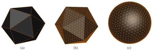
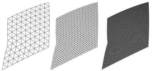
One method for achieving consistent cell areas is to initially approximate the globe with a regular polyhedron, such as a cube or icosahedron. The faces of this polyhedron are subdivided to create a hierarchy of repeatedly refined flat cells (i.e. triangle, quad, or hexagon) down to an arbitrary level of detail. The final (curved) cells are the result of un-projecting the resulting flat cells to the surface of the Earth, preferably using an equal-area projection (see Figure 2). Different types of initial polyhedrons and cell types have been used to create different grid structures used in various DGGSs (Mahdavi-Amiri, Alderson, and Samavati 2015). Although, the required type of grid system is dictated by the application's requirement, it causes some issues for interoperabilities among various DGGSs. Mahdavi-Amiri, Harrison, and Samavati (2016) provide a general framework for converting one hierarchical grid to another using simple transformations. This grid conversion is also fundamental for our client–server DE system.

Figure 2. An initial polyhedron (a), is refined (b), and then projected to the sphere (c).

Every cell within a DGGS is referenced by an index. This index is analogous to a latitude/longitude coordinate pair in that it indicates a particular location on the globe. Indices also serve as the entry point for data queries on a DGGS, since an index can be referenced to retrieve data from the area it represents. Several methods exist for producing indices, such as space-filling curve-based indexing, hierarchical indexing, and coordinate-based indexing; Mahdavi-Amiri, Samavati, and Peterson (2015) present various indexing methods in DGGS and conversions between them.

2.2. Focus+context visualization

In the fields of information and scientific visualization, Hauser generalized the common methods for discrimination between focus and context based on their degrees of importance (Hauser 2006). The use of a virtual lens to magnify foci is a common method for discriminating between focus and context (Hsu and Correa 2011; Taerum et al. 2006; Wang et al. 2011). Such visualizations draw their inspiration from preexisting techniques common to medical and scientific imagery, where the artist highlights areas of interest with magnified parts of an illustration (Hodges 2003). Our implementation uses a discontinuous undistorted technique (Taerum et al. 2006), rather than the continuous style (Hsu and Correa 2011; Wang et al. 2011), as the views are discrete and independent.

Packer et al. (Packer 2013; Packer, Hasan, and Samavati 2017) created a system allowing for multilevel focus+context visualization of layered tube-shaped structures with continuous artistic transitions between different levels of detail. However, unlike ours, their work does not support branching structures. Other related works include multifocal visualization of medical data by Ropinski et al. (2009), a multifocal, multilevel system by Cossalter, Mengshoel, and Selker (2013) for visualizing networks, a multifocal treemap visualization by Tu and Shen (2008), and multifocal and multicontext augmented reality systems by Mendez, Kalkofen, and Schmalstieg (2006) and Kalkofen, Mendez, and Schmalstieg (2007), respectively. Our approach primarily differs from these works in that it is based on view-dependent resource allocation derived from the viewing volumes of the foci.

Conventional DEs suffer from visualization difficulties stemming from the scales and distances involved in geospatial data. It is difficult to visualize regions that are vastly different in scale, as a single perspective is often insufficient. Viewing two or more distant areas at a high level of magnification is also problematic with a single point of view. Multilevel focus+context visualization technique of Hasan, Samavati, and Jacob (2014, 2016) and Hasan (2018) overcomes this limitation by providing multiple dynamic views of the data at customizable resolutions and perspectives. Their work produced a system that supports the exploration of large-scale 2D and 3D image data through a multilevel focus+context environment. The work is based upon a balanced wavelet transform (Hasan 2018; Hasan, Samavati, and Sousa 2015) of the dataset being visualized, and produces a tree structure where each level of magnification is available for further magnification by adding additional foci. Except for the root, each node in the tree can represent both focus and context in this environment and has varying degrees of interest (Card and Nation 2002) for directing resource allocations. Inspired by this work, our system uses virtual cameras to achieve multilevel focus+context visualization. However, our work applies to a curved Earth and relies on the server's available data for regions of interest (ROIs) as opposed to a multiresolution construction.

2.3. Geovisualization

One cannot meaningfully have a discussion of DE without referencing Google Earth (Google 2020). Google Earth supports a wide variety of data, and is possibly the best example of a photorealistic interactive 3D globe. It achieves a great level of data integration, though it lacks the analysis capabilities that are present in a DGGS.

With a similar set of features, Cesium (2020) is an open-source JavaScript library for web-based 3D globe visualization. It contains a wide variety of tools that span the spectrum from photorealistic visualization to plotting data on the globe. Their API allows for splitting the view of the globe, rendering different data on each pane. These panes, however only split the view between two different static sets of data. Our system improves on this by allowing the mixing of scales, moving distant locations closer together, and producing dynamic visualizations of data in real-time.

On the other hand, ArcGIS Online (ESRI 2020) is a web-based globe with more focus on data analysis compared to Google Earth and Cesium. This solution is part of a powerful analysis and visualization engine that supports a variety of data formats and sources. However, due to not being DGGS-based, some operations such as those benefiting from GPU-based hardware acceleration due to the straightforward correspondence between multiple large datasets at varying levels of resolutions offered by a DGGS, are difficult to run in real-time.

Finally, Global Grid Systems features a web-based globe that is constructed using our client-side system as a starting point (Global Grid Systems 2020). A wide variety of data can be imported and visualized, and a variety of cell-based analyses can be performed interactively because it is based on a DGGS.

3. Methodology

Our methodology for visualizing DE in a web browser is broken down into three separate topics: how we reference data, how we construct the view-aware DE, and how we build the data visualization system.

3.1. System overview

We present the implementation of a view-aware DE system capable of interactively displaying multiple simultaneous viewpoints, supporting multilevel focus+context visualization on the globe. It also supports several real-time data styling techniques that are designed to work efficiently on both the client and server. In our method, the client-side is responsible for triggering queries for missing data, managing the viewing area, and rendering various styles and effects. The server is responsible for generating data representations for DGGS cells in response to queries from clients. Only the data required for the current views and scales need to be processed, so the task of processing the datasets at their native resolution can be circumvented.

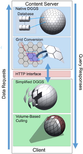
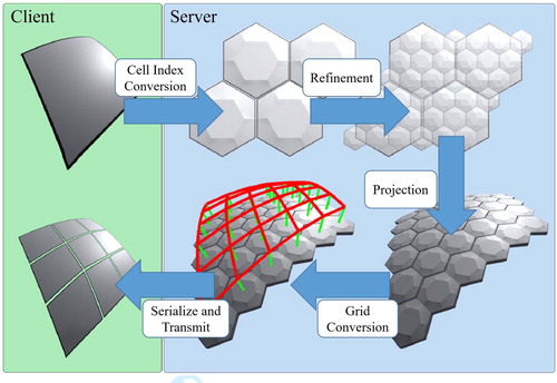
As illustrated in the visual synopsis of client and server responsibilities in Figure 3, tasks are divided between a server and one or more clients. Each client machine runs our client-side web application within a web browser, accessible via a URL. The client-side web application is programmed in JavaScript, so it runs in a variety of web browsers. It is functional in Microsoft Edge, Google Chrome, and even Chrome running on Android mobile devices. Our implementation makes use of WebGL, an API which is based on OpenGL ES for use in web browsers.

Figure 3. Overview of client and server responsibilities.

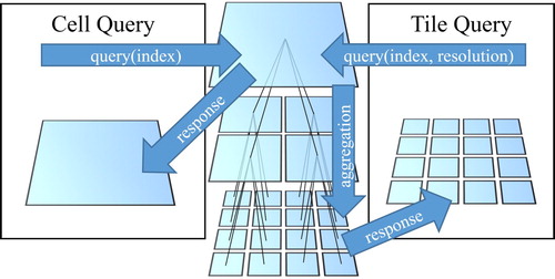
Although a DGGS is a very efficient framework for the storage and retrieval of data, queries sent over a network connection still have overhead. Because many thousands of cells need to be visible on the globe at a time for a visualization to be meaningful, this means that thousands of cells need to be queried. Individually requesting these cells is extremely impractical over a network. Therefore, data are shared between the client and server in the form of quadrilateral tiles composed of cells. These cells are the same as those used in the server DGGS, arranged into a quadrilateral tile through the use of an existing hierarchical grid conversion method (Mahdavi-Amiri, Harrison, and Samavati 2016). This hierarchical grid conversion for the case of hexagons to quadrilaterals is accomplished through the dual conversion method – the dual of a hexagonal grid is a triangular grid, where each vertex of a triangle corresponds to the centroid of a hexagon. The triangles of this dual grid are paired up to produce a quadrilateral grid. Next, to produce tiles, the cells in the quadrilateral grid are aggregated along the coordinate axes U and V of the parametric domain, as shown in Figure 3 and explained further in Section 3.3 (see Figure 6).

A tile is formed of cells sampled at a particular resolution and can be considered to be a special type of lower-resolution ancestor cell. Instead of containing a single datum, each tile contains an array of data values that correspond to its descendants' data at a higher level of detail. As shown in Figure 4, the process of requesting a tile from a DGGS is only slightly modified from the cell-querying process. Since many cells result from a single tile query, the cost of requesting these cells over the network is significantly reduced.

Figure 4. As opposed to a series of cell-based queries, a single tile-based query can request for all descendant cells at a desired resolution, reducing the cost of requesting those cells over the network.

The web application houses a hierarchy of tiles, which is created when the finer-detail data are requested and transmitted. Since these tiles are analogous to cells, this hierarchy serves as its own DGGS. We refer to this as the client DGGS. The client is responsible for determining which tiles need to be downloaded based on each tile's visibility within the current views and its size on the viewing screen. Each tile has its own unique index, which is used when the client sends queries for the desired data to the server. The server responds with data in tile form, which the client stores within the client DGGS.

The server has access to a database of geospatial datasets, referenced using the server DGGS. When the server is queried with the index of a given tile and a dataset, it samples the DGGS-referenced data and produces the result for the query as a tile. The query result takes one of two forms: the geometry of the cell being requested or a data texture representing the data thereupon.

Since tiles are collections of cells from the server DGGS, which can be sampled at different resolutions, they can contain a variable number of cells, as shown in Figure 5. A particular tile index has an accompanying resolution that indicates which level of detail the server DGGS was sampled at in order to produce it. Our system typically uses relatively low-resolution data for geometry, but high-resolution data textures to achieve a balanced trade-off between accuracy and performance.

Figure 5. A particular tile's geometry sampled at different levels of detail – here the cusp on the left edge of the tile is caused by the subdivision method applied to the dual hexagonal grid on the server DGGS.

3.2. Discrete Global Grid System

As discussed in Section 2, a core concept in DGGS is the idea that a cell with a particular index represents a physical piece of the Earth and is a bucket to which geospatial data may be assigned. Within a particular DGGS, the cell structure is immutable, giving every cell a known resolution, position, and size. When a dataset is stored into a DGGS, the data take on the same structure as the DGGS in which they are housed.

Though DGGSs often include complex indexing and projection schemes, these are not needed on the client-side if the server has the ability to serve cell geometry. Cell geometry, like other data, is provided to the client in the form of tiles. The two tests that the client needs to perform are tests for on-screen visibility and cell size, both of which may be performed on the geometry of the tiles. Using the server's ability to create and transmit tile geometry enables us to support interoperability with different DGGSs, since the client is not dependent upon a particular server-side DGGS and can interact with servers of a variety of data providers without modification.

3.3. Client–server DGGS

The client requests geometry and data tiles starting at the coarsest level of resolution and, in ROIs, requests refined tiles until an appropriate level of detail is acquired. This requires the client to be able to predict the indices of children cells, which is easily provided by the client-side hierarchy.

It is impractical to load full datasets onto the client due to limitations of memory and network throughput. To reduce the amount of data transmitted between the client and the server, we limit the data to only that which is required to render the globe from the current views. As views are changed (e.g. by zooming or panning) or added, the data needed to accommodate these views are requested and downloaded. The client requests the missing data from the server DGGS as shown in Figure 3. Since the exact size and resolution of cells are explicitly available from the client DGGS, they allow the client to send very specific queries to the server DGGS about which data are needed to complete a view.

In our client–server framework, the server transmits two types of information for rendering geospatial data on the client. The first type is globe geometry, consisting of 3D meshes that approximate the curved surface of the globe for a chosen tile, an example of which is shown in Figure 5. Because DGGS cells are indexed at various levels of resolution, the server DGGS can be queried in a manner capable of producing the mesh for a globe, in part or in whole, at a wide variety of resolutions. The second type of transmitted information is a preimage-tile of data that are to be visualized on the globe. To acquire these data, the client query references a data-source, an index, and a tile size, and the server responds with a sampling of data values within the corresponding cell. Since the tiles in both of these query types represent the same areas on the globe, their correlation is straightforward.

To reduce the processing load on the server, tasks such as rendering the globe and visualizing requested data are performed using client-side resources. Additionally, for the sake of efficiency, our server behaves in a stateless manner. Therefore, the client is also tasked with monitoring its downloaded tiles and for querying any missing data at its own discretion. To accomplish this, the client maintains a tree structure containing its downloaded tiles, which behaves as a client-side DGGS. Although the server and client DGGSs are closely connected, they do not necessarily have the exact same cell structure or hierarchy.

The DGGS underlying the server is typically not tuned for rendering or data transmission in a web-based environment. For example, as shown in Figure 3, the native DGGS (the PYXIS innovation 2020) on our server is built using hexagonal grids. Hexagons are a better choice for sampling data (Mahdavi-Amiri, Alderson, and Samavati 2015), but are not natively supported by graphics hardware. Thus, many systems require specialized methods for transmission and rendering.

Though the server in our implementation manages hexagonal cells, rectangular data are preferred on the client due to the ease of transmitting and rendering rectangular arrangements of data. Hierarchical grid conversion is a method by which hierarchical regular grids can be easily converted from one cell type to another (Mahdavi-Amiri, Harrison, and Samavati 2016). In this technique, triangular, quadrilateral, and hexagonal grids can be made interchangeable so that a system may utilize the various advantages of each, as needed. This conversion technique allows us to pack and convert hierarchical hexagonal grids into hierarchical quadrilateral grids with their own indexing methods. This packing is shown in Figure 6. The resulting indexing method allows us to build a tree of downloaded cells on the client-side, which can be efficiently traversed. Moreover, the resulting quadrilateral cells are compatible with the rendering pipeline, including shaders' 2D texture samplers.

Figure 6. An example client–server cell refinement process.

DGGSs use a variety of projection methods, typically area preserving, in order to map planar data to the surface of the Earth. To maintain interoperability with different DGGSs, our system relies on the server DGGS to perform the projection. This frees the client of the need to consider the often complex projection methods specific to any particular server. Therefore, the geometry and hierarchy of cells on the client DGGS depends on the structure of the server DGGS. A result of this is that the client cell hierarchy may not be perfectly congruent if the server DGGS is not congruent itself. To address this lack of congruency, when performing screen visibility tests, we use a bounding volume of the current cell that contains all descendant cells. Ensuring the bounding volume is sufficiently large is essential in order to prevent false-negatives in these tests.

4. View-aware DE and multiple views

One of the main goals of this work is to support multiple virtual cameras for DE applications. Each camera is responsible for the live creation of one view of the DE. In this Section, we show how our system can support multiple simultaneous views of the globe and how this enables multilevel focus+context visualization. We also explain how our system manages appropriate levels of detail and determines what new data to download.

4.1. View-aware DE

To render a high-detail DE in real-time, a system has to be discerning about its allocation of resources. A complete high-detail globe is impractical to download or render in real-time. Instead, our client-side globe tracks the extant cameras and adapts to each of them. Such adaptation ensures that the portions of the globe that are rendered are those that can be seen by the camera and are of appropriate resolution. Therefore, we base our method on two factors – determining what parts of the globe are visible to a camera, and determining the appropriate level of detail that should be presented to a camera.

For a given camera, we determine which tiles are outside of the view camera frustum so that they can be ignored by the rendering process. The tree hierarchy of the client DGGS, introduced in Section 3.3, is useful for determining the visibility and scale of portions of the globe. Additionally, to determine the appropriate level of detail, we determine the ratio of visible data samples in a tile to the number of screen pixels that it covers. To approximate the size of each tile on the screen, a bounding volume is calculated. In our implementation, we use bounding spheres, though other types of volumes are possible.

After projecting the bounding volume into screen space via the camera, we estimate the number of pixels that the tile covers on the screen by calculating how many pixels are covered by the bounding volume. By measuring the approximate ratio of cells in the tile to the number of screen pixels the tile occupies, we calculate a factor that determines whether the tile's resolution is appropriate for the current view. If this ratio is lower than a certain threshold, the tile is too large on the screen and is then replaced with its children. On the other hand, if this ratio is high, the tile is too small and contains data that are sub-pixel on the screen. In this case, its rendering costs exceed its benefit to the visualization, so it (and its siblings) are replaced with the parent tile instead.

The bounding volumes are also used to determine whether a particular tile is visible to the camera. If the bounding volume of a tile does not intersect the viewing frustum, the tile and its children are not visible. It is this property that makes the culling of the globe efficient, as entire branches of the tree can be quickly pruned without the need to test every individual tile in each branch.

This culling process can run many times between frames of animation. This allows the globe to adapt to a multitude of concurrent cameras. We render the cameras sequentially, adapting the globe to each in turn just before it is rendered.

4.2. DGGS tree traversal

In our method, the processes of rendering the globe and queuing the download of missing data are combined into a single traversal of the tree structure that represents the tile hierarchy of the client DGGS.

Since our client starts with very little information about the DGGS it is about to use, it requires a starting set of data. Therefore, when first created, the client requests from the server a list of indices for the tiles at the coarsest resolution and queues these tiles for download. Once the geometry for these tiles is received, it becomes possible to determine each tile's size and location, and traverse the client's DGGS tree for each camera. Algorithm 1 outlines this traversal. This algorithm recursively produces a list of tiles that should be rendered for a particular camera for a single frame, while it queues the download of any missing data. Since these downloads are an automatic by-product of our visibility checks, any camera in the scene can trigger the globe to download additional data as needed.

Algorithm 1: Depth-first tree traversal for requesting data and culling.

4.3. Multiple views and multilevel focus+context

One of the challenges of this work is to create a visualization and rendering framework capable of showing multiple and diverse geospatial datasets in the context of Digital Earth. As discussed in Section 2.2, multilevel focus+context is a method that may address this challenge.

While the techniques we have described thus far are sufficient to create multilevel focus+context, some challenges remain. Our system supports dynamic multilevel focus+context visualization, in which multiple ROIs can be viewed simultaneously, regardless of proximity or difference in scale. These different views form a multilevel, multiview hierarchy and provide context cues where applicable, allowing a viewer to easily identify the areas or different types of data being emphasized.

We extend the method proposed by Hasan, Samavati, and Jacob (2014, 2016) and Hasan (2018) for the creation and management of our multilevel focus+context visualization hierarchy for flat images to work with curved Earth models. In our work, the view-aware DE reacts to cameras to perform view culling and provide a comparable functionality. Thus, to extend multilevel focus+context visualization to our view-aware DE, we associate regions of interest (ROIs) with interactive cameras, interacting with datasets in varying resolutions indexed by the client DGGS. Our visualization is achieved as follows.

Initially, a new ROI can be chosen on the globe view interactively. This may be achieved in a variety of ways, such as by sketching strokes or by drawing a bounding box. A new camera is then created in the scene so that its viewable area matches the chosen ROI. Next, a magnified view of the ROI as viewed by the new camera is rendered separately on the screen. Finally, we render semitransparent connections between the chosen ROI and its magnified view. In the focus+context creation scenario thus described, the ROI is located on the initial globe view, which provides contextual information. Additionally, a magnified view of an ROI can recursively serve as the context for new ROIs. This allows the system to facilitate the creation of a multilevel focus+context visualization hierarchy (see Figure 1, for example).

Each of the newly created cameras is dynamic and can be controlled interactively. Alternatively, these cameras may be moved or animated procedurally. For example, a camera can be made to follow the orbit of a satellite, providing a live view from the satellite's point of view.

As discussed in Section 4.1, our DE system adapts to the views of the cameras, showing the globe from each view in the scene with an appropriate level of detail. Because downloading new data is also a by-product of this process, creating, moving, or zooming any of these cameras requests missing data where applicable. As this process only downloads missing data, regions viewed by two cameras at the same level of detail do not require the data to be acquired twice.

Internally, the cameras form a tree hierarchy, the root camera having the responsibility of rendering the globe to the main canvas. Any other camera is assigned a WebGL viewport, which represents the focus. All non-root cameras are also assigned a parent camera. A camera is the parent of all cameras whose ROIs appear within its focus. Thus, if an ROI is selected on the main view of the globe, a new camera is created as a child of the root camera, and its ROI is drawn on the main view. If an ROI is then selected within the viewport of this new camera, a third camera is created. This newest camera is the child of the previous, with its ROI being drawn within its parent's viewport.

4.4. Multilevel focus+context interface

To support multilevel focus+context visualization, we have to be able to place new cameras dynamically in positions that represent an increase of detail. This happens as the result of a user interaction within the browser. When an interaction event is detected, we check to see if it was produced within an existing viewport area. If the interaction is within a viewport, a new camera is produced that is a child of the viewport's associated camera, otherwise the new camera is a child of the original scene camera. This relationship defines a hierarchy for the various cameras in the scene.

In order to position the new camera in the scene, a ray is cast from the interaction coordinates into the 3D scene. The new camera is then positioned at some point along this ray, proportional to the zoom level desired. Alternatively, the new camera could be placed at a distance to the globe identical to its parent's, but with an altered Field of View (FOV) to produce zoom instead. These camera placements produce zoomed-in views that visually emulate the lens effect that is common in focus+context.

Once the cameras are placed, the ROIs need to be rendered, along with their connections to the foci. Cameras in 3D environments can be considered to possess a virtual rendering plane, somewhat like the film in a real-world camera. This virtual plane can be placed anywhere within that particular camera's viewing frustum. To aid with the visual association of where the camera is, and what it is looking at, our experiments reveal that a good approach is to pick a viewing plane that is very close to the surface of the globe. This produces a viewing plane that is large and also very close to the area on the Earth that it is viewing. Choosing a large viewing plane is beneficial because it is more likely to be visible if the parent view differs greatly in scale. The plane's proximity to the surface draws a strong correlation between the camera and the area it is viewing.

5. Performance considerations

The performance of the proposed system is a major factor in its design, as there are various interacting constraints. For our solution to work in practice, the server should be efficient, and ideally should benefit from technologies that scale well to large numbers of clients. The client's limitations also need to be considered, as caching large amounts of data within a web browser is not practical; only the RAM of the client machine should be considered available. Our system achieves a balance between these constraints while providing benefits to rendering and interactivity over current technologies. Here, we examine the performance characteristics of the main areas where performance bottlenecks could occur. These areas are the tree culling algorithm, which needs to be efficient in order to support multiple views, and the data encoding and caching mechanisms. These factors impact memory, network, and CPU usage on both the client and server.

5.1. Tree hierarchy and culling

Fast and appropriate culling is vital to this work. In order to render multiple simultaneous live views of a globe in real-time, we need to produce visible geometry that is suitable for fast rendering. Additionally, this decision needs to be quick as it has to be made for each camera in the scene. We expect our spatial tree to be able to cull data very quickly. We validated this hypothesis experimentally using Algorithm 1. Rendering 10 concurrent cameras, we typically maintained approximately 60 frames per second, with frame time between 13 ms and 20 ms. We also tested a render made up of tiles predominantly at the 8th resolution. At this resolution, it would take 430,467,210 quadrilaterals to fully cover the globe. As shown by the examples in Table 1, our system only needs to consider 495 of these quadrilaterals in the process of determining the 67 required for this rendering. Table 1 additionally shows the average time taken to download the tiles checked for visibility at each resolution, where the reported time is an average of 15 test runs.

Table 1. Comparison between the number of tiles checked for visibility, tiles visible to a camera, the total number of DGGS tiles at various resolutions, and average time taken to download the tiles checked for visibility. Server and client DGGS prototypes were equipped with 3.2 GHz Intel® Core™ i7-8700 and 2.6 GHz Intel® Core™ i7-6700 CPUs, respectively, and 16 GB of RAM each.

Level of resolution	Checked tiles	Visible tiles	Total tiles	Time to download checked tiles (ms)
1	90	45	90	670
2	153	78	810	976
3	279	41	7290	1869
4	315	34	65,610	2172
5	351	33	590,490	2340
6	414	56	5,314,410	2550
7	486	56	47,829,690	2950
8	495	67	430,467,210	3323

A drawback to using downloaded globe geometry to populate a spatial tree is that lower resolution regions must be downloaded before their higher resolution children. However, the overhead of a single parent tile is shared by all of its children. Thus, on average, the overhead is $t\cdot \sum _{r=1}^R\frac{1}{n^r}$, where t is the number of visible tiles and n is the number of children tiles in the multiresolution scheme, and R is the level of resolution for a viewed area. Experimentally, we find that this is close to the trend in our system. From the example above, the 67 visible quadrilaterals required only 7 tiles from coarser resolutions to support them within the hierarchy, close to the 8.37 we would expect.

5.2. Data transmission and encoding

Our primary method of encoding data is in the form of data textures. This encoding system uses the indexing scheme of Mahdavi-Amiri, Samavati, and Peterson (2015) and Mahdavi-Amiri, Harrison, and Samavati (2016), which can produce square textures wherein each texel represents a single tile of the DGGS from which it was sampled. In essence, the data textures are used as a method of batching a series of tiles for transmission. With this in mind, next we compare this process against the transmission of the hierarchical DGGS data if it were transmitted in some other format.

If the data were, for example, batched as a hierarchy of hexagons rather than data textures corresponding to the quadrilateral regions used in our client-side DGGS, the total amount of data sent would be similar. The hierarchy would, however, represent a region that is difficult to access within a shader. It would be possible to run the grid conversion algorithm (Mahdavi-Amiri, Samavati, and Peterson 2015; Mahdavi-Amiri, Harrison, and Samavati 2016) on the client to take some load off the server. We considered this model, but opted for the server-side grid conversion largely due to the asymmetry in the environments between client and server. The server has the ability to work with large hard drives and sizable caches, whereas a browser-based client is largely limited to just RAM. This allows the server to access small sections of a large dataset to handle the grid conversions per-request. A client-side grid conversion would likely require the client to maintain a memory-resident cache of cellular DGGS data as well as an entirely duplicate set of render-friendly rectangular textures and geometry.

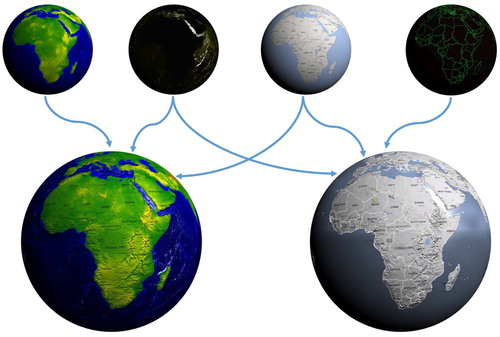
Our method of packing datasets into data textures is not exclusively used for improving the visual results; it also produces some considerable performance benefits. A particular dataset can be used for different purposes by different users. On one visualization, an elevation dataset may be used for shading terrain, whereas on another it could be used to colour a topographic map. To meet the demands of both clients, the server only needs to generate a single texture. This result can be used by both clients for their respective visualizations (see Figure 7, for example). This considerably improves the server's efficiency as it is able to cache results from a wide variety of visualizations with a relatively small number of textures.

Figure 7. Data textures shared between different visualizations (data sources: 1, 2, 4).

Similar benefits exist on the client-side as well. Some data textures on the globe can be reused between visualizations. If the client switches between two renderings where geopolitical boundaries are visible, the textures defining these boundaries do not need to be re-downloaded, even if they are styled differently. Our interactive data styling method utilizes this property. Since styling is purely a choice on how the textures are converted into colours on the screen, no new request for data is sent to the server when styling parameters are altered.

Though web caching works well with our system, there is a second type of caching that additionally helps with the overall server performance. A web cache will only get a successful cache hit on a texture if all four of the image channels match a previous request and if they were normalized and quantized with the same functions. Cache hits are therefore most probable if the images contain data which are commonly used together. To improve cache efficiency further, we also cache the individual data layers before they are packed into data textures for transmission to clients. This allows for cache hits even when a client asks for data arranged in a layer order not previously requested.

6. Data styling and visualization

In this section, we show how our work addresses several of the issues of web-based visualizations of data on the globe. Since an interface built atop a DGGS provides access to many datasets, we have been able to produce a variety of results using our implementation. Each render in this section is the product of multiple datasets used in a variety of manners. Results are divided into two subsections: the first subsection highlights the results of using data textures to produce visualizations beyond RGB values, and the second subsection focuses on results using multilevel focus+context visualization.

Data visualization is at its most useful when it can show us multiple data attributes at the same time. When the toolset is limited to only RGB texture values, colours can be quickly expended. This problem is compounded in datasets with pre-assigned colour codings. When blending such datasets using a preset colour legend, collisions between colours are both very likely, and difficult for a user to resolve. Since our system separates colour from the data, these conflicts can be altered in real-time through interactive styling and visualization. Furthermore, the visualization has access to a wider set of rendering parameters (e.g. lighting attributes) that yield effects that are more than just standard RGB texturing.

6.1. Data styling

Providing an interface that can map data to various rendering parameters allows us to produce a variety of complex results. Also, since these parameters are commonly used by the shaders within the rendering API, we produce 3D scenes with consistent lighting throughout. This is useful as it allows for digital globes to be used in a wider variety of applications. Rather than being confined to a purpose-built application designed to render only the Earth, the globe can be integrated seamlessly into visualizations that include other objects within the 3D space.

The ability to customize how light interacts with the globe is a useful added feature in itself. In Figure 8, topographical data are shown on the globe. In this case, it allows for the inclusion of a map dataset, which would normally interfere or obscure parts of the visualization, without compromising the information being conveyed. This visualization was produced by filtering a map dataset to highlight roads and labels, meanwhile suppressing features like lakes and parkland, then assigning the result to rendering parameter responsible for normal perturbation.

Figure 8. Topographical visualization with landmarks included as a normal perturbation to give location context (data sources: 1, 4).

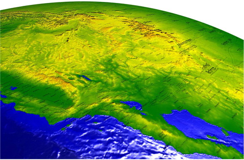
Rendering effects can be used to increase the perception of variations in a dataset, as shown in Figure 9(a). Variations in ocean depth, when visualized as colour gradients, can convey some information. However, since our own sense of detail in the real world often takes into account variations of lighting on a surface, these details stand out more when they interact with a scene's lighting model.

Figure 9. Various client-side data styling scenarios. (a) Artistic texture and styling emphasizing topography and bathymetry (data sources: 1, 3). (b) Map textures and embossed political boundaries (data sources: 1, 2, 4). (c) Population data and political boundaries as light-emitting textures (data sources: 1, 2, 5).

Figure 9(b) illustrates how lighting can be used to elevate the importance of particular features in a visualization. In this image, political boundaries are given some slight depth and light emission, allowing them to stand out from other map features, such as roads or parks, which are also shown but not highlighted. The textures for topographic and bathymetric shading are reused from Figure 9(a) and do not need to be re-downloaded if the client transitions from one to the other.

Figure 9(c) illustrates a more extreme use of light and shadow. In this visualization, population density is made to stand out from the rest of the map by moving the light source. Light emission allows a surface to produce some degree of light, effectively becoming glow-in-the-dark. Thus, interaction with the scene's light source acts as a method of switching between or blending multiple visualizations.

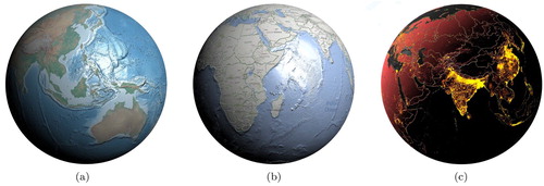
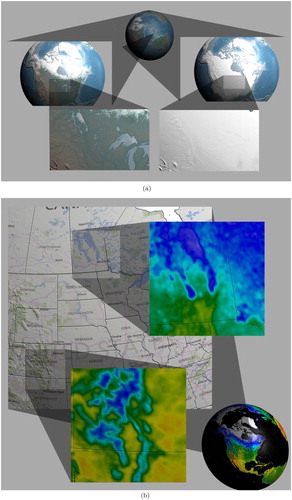
Figure 10 shows the versatility of styling matrices. The three types of visualization shown use the same four underlying data textures on the globe. Styling matrices can be used to produce a variety of visualizations, emphasizing different aspects of the data. These styling matrices may be blended or altered in real-time on the client, producing smooth animation from one style to another. Since these styling calculations are run on the client, these changes are made without any additional interaction with the server.

Figure 10. Three different visualizations of the same data but using different styling matrices (data sources: 1, 2, 3, 4, 5).

Conventional shaders used in applications such as video games typically dedicate one texture per lighting parameter, such as having a specular map, a texture map, a bump map, and so on. Our shaders needed to loosen this constraint, so they employ a styling matrix to remap each texture dynamically. This matrix is provided to the shader so that it may transform the sampled values for the provided textures, and create a set of virtual samples, as if we were actually using a specular map, a texture map, etc. The rest of the shader runs much like conventional ones. Simple changes to this styling matrix allows for considerable manipulation of the meanings of each input texture.

6.2. Multilevel focus+context visualization

Datasets vary by location and in scale considerably, and this presents an obstacle to visualization. Figure 11(a) shows road networks for Alberta and Nova Scotia. Unfortunately, if one were to attempt to compare the differences in the arrangements of these road networks with a typical single-view visualization, they would be forced to pan back and forth between the areas. A single view that captures both datasets is too distant to display enough detail, and a closer view is incapable of displaying both sets of features.

Figure 11. Canadian road networks in Alberta and Nova Scotia (data sources: 1, 8, 9). (a) These two road networks in Alberta and Nova Scotia cannot be viewed at high detail simultaneously without special techniques due to their distance and difference in scale. (b) Effective comparison of the road networks in Alberta and Nova Scotia utilizing multilevel focus+context visualization.

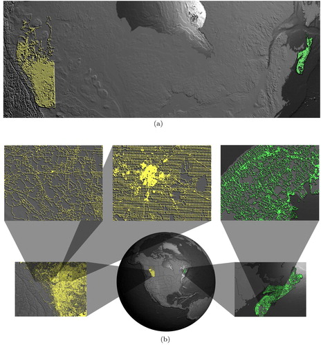
To confront this obstacle, as discussed in Section 4.3, our view-aware DE is capable of presenting appropriate levels of detail to multiple views at the same time, with little overhead. We chose to demonstrate this functionality through an implementation of multilevel focus+context visualization on DE. Figure 11(b) clearly shows the different patterns present in these datasets, as an appropriate level of detail is possible. Our system also facilitates easy and effective comparisons of ROIs in very distant locations or at very different scales. Despite the scales and distances involved, the respective contexts allow a user to easily perceive scale and location of the data being viewed.

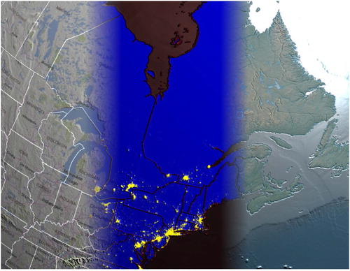
In Figure 12(a), we display the population densities of a few ROIs on the Earth. In a single-view DE visualization, it would not be possible to show this level of detail for areas so far apart.

Figure 12. Multilevel focus+context visualization on the globe. (a) Population densities in different parts of the world (data sources: 1, 2, 5). (b) Calgary water bodies and flood projection (data sources: 4, 10, 11).

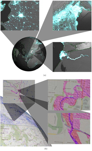
Our multi-view visualizations are also compatible with all of the benefits of our data integration and visualization systems. In Figure 12(b), we illustrate another benefit of a client-side rendering of data. Here we present a flood warning dataset, which originally comes in the form of vectors. When overlaying such a dataset on a map, the result can be confusing because the colours used by the dataset may conflict with those employed by the map. To avoid such confusion in this visualization, we apply an animated water-like ripple to the flood dataset, allowing it to stand out strongly against the background map. As all of our views are real-time, these regions animate within the foci and on the base globe simultaneously.

The views themselves may also interact with the data rendering techniques, as shown in Figure 13. In these visualizations, each globe view may possess its own styling parameters. Thus, focus+context visualizations can be used for side-by-side analysis of a single location, or as a method of browsing other styling options for the chosen datasets.

Figure 13. Multilevel focus+context visualizations which influence dataset styling. (a) Visualization comparing freezing point in winter versus spring (data sources: 1, 3, 6). (b) Mean temperatures for 2015, using a map dataset for context (data sources: 1, 4, 6).

7. Conclusion and future work

Our presented globe-based multiresolution DE overcomes several major challenges in the visualization of large geospatial datasets, particularly in the areas of data integration, versatility of visualization, effective user-interactions, and performance.

Data integration is a difficult task in many areas of geospatial visualization. Our presented system overcomes this difficulty by the use of a novel client–server DGGS that provides an interface to data that is free of conflicting projections or coordinate systems. The equal-area nature of DGGS cells also contributes to an environment where data can be easily compared and combined without expensive analysis.

The versatility of visualization in our presented system can be largely attributed to the consistent manner in which we treat various geospatial datasets – as data textures. Our rendering techniques process an array of data textures, wherein each texel represents the same location and area as its equivalent in another data texture, or channel therein. This enables the use of GPU-based hardware acceleration on the client-side, where a shader performs the required operations on multiple data textures. The ability to combine these data textures on the shader allows for fast and diverse client-side styling, and even animations between different styles.

By extending the multilevel focus+context visualization technique to curved Earth models through the concurrent and coordinated use of multiple cameras, our presented system provides an effective context-aware method to interact with and navigate through large multiscale geospatial datasets. While allowing for such multi-view visualisation, our presented system remains interactive by dynamically adapting to the views of the cameras within the scene – only the data viewable by a camera are requested for download, and at a level of detail that is appropriate for its proximity to the surface of the globe.

Relevant future works include the expansion of this system to handle large-scale time-varying data. An example of this would be smoothly and interactively traversing through years of Landsat data. We are also interested in the exploration of data-driven procedural content on the surface of the globe, such as the generation of 3D forests with high levels of detail. Additionally, we would prefer extending the set of data styling functions for use on the client-side. Further integration of the rendering process into DGGS is also a point of future interest, as we believe that a GPU-based referencing scheme for DGGS is inevitable, and would allow the grid to be drawn directly without the need for intermediate geometry. We are also interested in the inclusion of volumetric data within a web-based DE, as this would allow for the modeling and visualization of weather and subterranean features.

Credits for datasets

(1)	NOAA: 2-Minute Global Relief, www.ngdc.noaa.gov
(2)	ESRI: World Political Boundaries, www.esri.com
(3)	Natural Earth: Vector and Raster Map Dataset, www.naturalearthdata.com
(4)	Microsoft: Bing Maps, www.bing.com
(5)	Columbia University: Gridded Population of the World, sedac.ciesin.columbia.edu
(6)	NASA: Land Surface Temperature, neo.sci.gsfc.nasa.gov
(7)	NASA/USGS: Landsat 8, landsat.usgs.gov
(8)	Highway Geomatics Section (HGS), Alberta Transportation: Alberta Road Network, geodiscover.alberta.ca
(9)	Natural Resources Canada: Nova Scotia Road Network, www.nrcan.gc.ca
(10)	Statistics Canada: Canadian Inland Lakes and Rivers, www.statcan.gc.ca
(11)	City of Calgary: 1:100 Year Flood Map, www.calgary.ca

Acknowledgments

We would like to thank Idan Shatz, Ali Mahdavi-Amiri, and Perry Peterson for their insightful discussions and Troy Alderson for his editorial comments.

Disclosure statement

No potential conflict of interest was reported by the author(s).

Additional information

Funding

This research was supported in part by the National Science and Engineering Research Council (NSERC) of Canada and the PYXIS innovation inc.

References

- Alderson, Troy, Ali Mahdavi-Amiri, and Faramarz Samavati. 2016. “Multiresolution on Spherical Curves.” Graphical Models 86: 13–24.
- Alderson, Troy, Matthew Purss, Xiaoping Du, Ali Mahdavi-Amiri, and Faramarz Samavati. 2020. Digital Earth Platforms, 25–54. Singapore: Springer Singapore.
- Card, Stuart K., and David Nation. 2002. “Degree-of-Interest Trees: A Component of an Attention-Reactive User Interface.” In Proceedings of the Working Conference on Advanced Visual Interfaces, New York, USA, 231–245. ACM.
- Cesium. 2020. “Cesium, An Open-Source JavaScript Library for World-Class 3D Globes and Maps.” https://www.cesiumjs.org
- Cossalter, Michele, Ole J. Mengshoel, and Ted Selker. 2013, February. “Multi-Focus and Multi-Level Techniques for Visualization and Analysis of Networks with Thematic Data.” In Proceedings of the SPIE Conference on Visualization and Data Analysis, Burlingame, CA, USA, Vol. 8654, 16–30, 865403.
- ESRI. 2020. “ArcGIS.” https://www.arcgis.com
- Gil, Yolanda, Suzanne A. Pierce, Hassan Babaie, Arindam Banerjee, Kirk Borne, Gary Bust, and Michelle Cheatham, et al. 2018. “Intelligent Systems for Geosciences: An Essential Research Agenda.” Communications of the ACM 62 (1): 76–84.
- Global Grid Systems. 2020. “Global Grid Systems.” https://globalgridsystems.com
- Goodchild, Michael F. 2000, March 26–28. “Discrete Global Grids for Digital Earth.” In Proceedings of the 1st International Conference on Discrete Global Grids, Santa Barbara, CA, USA, 69–77.
- Goodchild, Michael F. 2018. “Reimagining the History of GIS.” Annals of GIS 24 (1): 1–8.
- Google. 2020. “Google Earth.” https://earth.google.com/web
- Hasan, Mahmudul. 2018. “Balanced Multiresolution in Multilevel Focus+Context Visualization.” PhD diss., Department of Computer Science, University of Calgary, Alberta, Canada.
- Hasan, Mahmudul, Faramarz F. Samavati, and Christian Jacob. 2014, October 6–8. “Multilevel Focus+Context Visualization using Balanced Multiresolution.” In Proceedings of the International Conference on Cyberworlds, 145–152. IEEE Computer Society.
- Hasan Mahmudul, Faramarz F. Samavati, and Christian Jacob. 2016. “Interactive Multilevel Focus+Context Visualization Framework.” The Visual Computer 32 (3): 323–334.
- Hasan Mahmudul, Faramarz F. Samavati, and Mario C. Sousa. 2015. “Balanced Multiresolution for Symmetric/Antisymmetric Filters.” Graphical Models 78: 36–59.
- Hauser, Helwig. 2006. “Generalizing Focus+Context Visualization.” In Scientific Visualization: The Visual Extraction of Knowledge from Data, edited by Georges-Pierre Bonneau, Thomas Ertl, and Gregory M. Nielson, 305–327. Berlin: Springer.
- Hodges, Elaine R. S. 2003. The Guild Handbook of Scientific Illustration. Hoboken, NJ: John Wiley and Sons.
- Hsu, Wei-Hsien, Kwan-Liu Ma, and Carlos Correa. 2011. “A Rendering Framework for Multiscale Views of 3D Models.” In Proceedings of the SIGGRAPH Asia Conference, New York, USA, 131:1–131:10. ACM.
- Kalkofen D., E. Mendez, and D. Schmalstieg. 2007. “Interactive Focus and Context Visualization for Augmented Reality.” In IEEE/ACM International Symposium on Mixed and Augmented Reality, November, 191–201. IEEE.
- Kooima R., J. Leigh, A. Johnson, D. Roberts, M. SubbaRao, and T. A. DeFanti. 2009. “Planetary-Scale Terrain Composition.” IEEE Transactions on Visualization & Computer Graphics 15: 719–733.
- Liu, Zhen, Tim Foresman, John van Genderen, and Lizhe Wang. 2020. Understanding Digital Earth, 1–21. Singapore: Springer Singapore.
- Mahdavi-Amiri, Ali, Troy Alderson, and Faramarz Samavati. 2015. “A Survey of Digital Earth.” Computers & Graphics 53 (Part B): 95–117.
- Mahdavi-Amiri, Ali, Troy Alderson, and Faramarz Samavati. 2019. “Geospatial Data Organization Methods with Emphasis on Aperture-3 Hexagonal Discrete Global Grid Systems.” Cartographica: The International Journal for Geographic Information and Geovisualization 54 (1): 30–50.
- Mahdavi-Amiri, Ali, Erika Harrison, and Faramarz Samavati. 2016. “Hierarchical Grid Conversion.” Computer-Aided Design 79: 12–26.
- Mahdavi-Amiri, Ali, Faramarz Samavati, and Perry Peterson. 2015. “Categorization and Conversions for Indexing Methods of Discrete Global Grid Systems.” ISPRS International Journal of Geo-Information4 (1): 320–336.
- Mendez E., D. Kalkofen, and D. Schmalstieg. 2006. “Interactive Context-Driven Visualization Tools for Augmented Reality.” In IEEE/ACM International Symposium on Mixed and Augmented Reality, October, 209–218. IEEE.
- Packer, Jeffrey F. 2013. “Focus+Context via Snaking Paths.” Master's thesis, Department of Computer Science, University of Calgary, Alberta, Canada.
- Packer, Jeffrey F., Mahmudul Hasan, and Faramarz F. Samavati. 2017. “Illustrative Multilevel Focus+Context Visualization Along Snaking Paths.” The Visual Computer 33 (10): 1291–1306.
- Purss, M. B. J., R. Gibb, F. Samavati, P. Peterson, and J. Ben. 2016, July 10–15. “The OGC® Discrete Global Grid System core standard: A framework for rapid geospatial integration.” In 2016 IEEE International Geoscience and Remote Sensing Symposium (IGARSS), Beijing, China, 3610–3613.
- the PYXIS innovation. 2020. “How PYXIS Works.” http://www.pyxisinnovation.com
- Ropinski, Timo, Ivan Viola, Martin Biermann, Helwig Hauser, and Klaus Hinrichs. 2009. “Multimodal Visualization with Interactive Closeups.” In Proceedings of the Theory and Practice of Computer Graphics Conference, 17–24. Eurographics Association.
- Taerum T., Mario Costa Sousa, Faramarz F. Samavati, S. Chan, and Joseph Ross Mitchell. 2006. “Real-Time Super Resolution Contextual Close-Up of Clinical Volumetric Data.” In Proceedings of the Joint Eurographics – IEEE VGTC Symposium on Visualization, May 8–10, 347–354. Eurographics Association.
- Tu, Ying, and Han-Wei Shen. 2008. “Balloon Focus: A Seamless Multi-Focus+Context Method for Treemaps.” IEEE Transactions on Visualization and Computer Graphics 14 (6): 1157–1164.
- Wang, Yu-Shuen, Chaoli Wang, Tong-Yee Lee, and Kwan-Liu Ma. 2011. “Feature-Preserving Volume Data Reduction and Focus+Context Visualization.” IEEE Transactions on Visualization and Computer Graphics 17 (2): 171–181.