Improvement of microwave emissivity parameterization of frozen Arctic soils using roughness measurements derived from photogrammetry

ABSTRACT

Soil emissivity of Arctic regions is a key parameter for assessing surface properties from microwave brightness temperature (Tb) measurements. Particularly in winter, frozen soil permittivity and roughness are two poorly characterized unknowns that must be considered. Here, we show that after removing snow, the 3D soil roughness can be accurately inferred from in-situ photogrammetry using Structure from Motion (SfM). We focus on using SfM techniques to provide accurate roughness measurements and improve emissivity models parametrization of frozen arctic soil for microwave applications. Validation was performed from ground-based radiometric measurements at 19 and 37 GHz using three different soil emission models: the Wegmüller and Mätzler [1999, TGRS] model (Weg99), the Wang and Choudhury [1981, JGR] model (QNH), and a geometrical optics model (Geo Optics). Measured and simulated brightness temperatures over different tundra and rock sites in the Canadian High Arctic show that Weg99, parametrized with SfM-based roughness and optimized permittivity $(\epsilon )$, yielded an RMSE of 3.1 K ($R^2=0.71$) for all frequencies and polarizations. Our SfM based approach allowed us to measure roughness with 0.1 mm accuracy at 55 locations of different land cover type using a digital camera and metal plates of know dimensions.

KEYWORDS:

• Surface roughness
• microwave remote sensing
• frozen Arctic soil
• SfM photogrammetry

1. Introduction

Most research on natural soil reflectivity focuses on soil moisture retrievals at L-band (reviewed by Wigneron et al. 2017) or higher frequencies (Njoku et al. 2003). Soil permittivity values are key parameters that allow retrieval of soil moisture using soil emissivity models such as those developed by Zhang et al. (2010) and Mironov et al. (2017). However, active and passive microwave dielectric sensitivity to soil moisture is strongly reduced by surface roughness that must be known or derived in the retrieval processing. During Arctic winter, surface parametrization is more difficult due to the presence of snow cover, and significant lingering uncertainties remain, specifically regarding required soil characteristics that are challenging to quantify in the Arctic.

Large scale monitoring of snow properties in the Canadian Arctic using both active and passive microwave has been conducted in the past (reviewed by Saberi et al. 2020; Shi, Xiong, and Jiang 2016) using measurement inversions based on radiative transfer models (Picard et al. 2013; Royer et al. 2017). These models must consider contributions from both snow and ground to simulate total backscatter or emission, particularly over northern areas with shallow snow cover (Roy et al. 2013; Derksen et al. 2014; Montpetit et al. 2018). Several soil microwave models integrated into the Snow Microwave Radiative Transfer Model (SMRT) (Picard, Sandells, and Löwe 2018) allow simulation of soil emissivity, but many uncertainties are associated with the permittivity and roughness of frozen ground (Montpetit et al. 2018). Models used for forward retrievals of soil parameters with satellite remote sensing are usually semi-empirical for the purposes of simplicity. For instance, the Soil Moisture Active and Passive mission (SMAP) retrieval algorithms use the QNH model, named for its parameters, Q, N, and H, to simulate surface reflectivity following Wang et al. (1983) and Wang and Choudhury (1981). More recently, the parameters in the QNH model were optimized by different studies (Wigneron, Laguerre, and Kerr 2001; Lawrence et al. 2013; Montpetit et al. 2015). Of particular relevance, the roughness parameters needed for the QNH model consist of effective parameters that were found to have smaller values than the actual physical measurements (Tsang and Newton 1982; Ulaby, Moore, and Fung 1982). Another semi-empirical model (Wegmüller and Mätzler 1999), developed for a wider range of applications (1–100 GHz), was derived from the QNH model using a simpler Kirchhoff approximation (Mo, Schmugge, and Wang 1987). Montpetit et al. (2018) parametrized permittivity and roughness using the Wegmüller and Mätzler (1999) semi-empirical model by optimizing surface-based radiometer multi-angle measurements of frozen soils in a subarctic environment in northern Québec, Canada, for higher frequencies (19 and 37 GHz) needed for snow application. Theoretical permittivity can also be calculated using the two models stated earlier: (Zhang et al. 2010; Mironov et al. 2017).

Surface reflectivity can be solved analytically using the Kirchhoff approximation or the Small Perturbation Method (SPM) with its associated bi-static coefficient. However, this requires a more detailed knowledge of the surface to determine which regime of scattering is involved (e.g. rough surface with geometrical optics). Other analytical solutions like Integral Equation Model (IEM or AIEM) (Fung 1994) can be used to simulate surface reflectivity. Finally, numerical methods solving Maxwell's equation using the Finite Element Method (FEM) or Method of Moments (MoM) (Lawrence et al. 2011; Tsang et al. 2013, 2017) can be used to calculate the scattered electric field from a rough surface, but they are more complex and computationally intensive than the models described above.

Another issue in soil microwave modeling is how to measure the soil roughness and link it to microwave sensitivity. The most common parameter used to describe roughness is height standard deviation (${\sigma }_H$), but it can also be described by horizontal correlation length $(l_c)$. Soil roughness parameters can be measured directly using a needle profiler (Trudel et al. 2010) or indirectly with terrestrial laser approaches (Martinez-Agirre et al. 2019; Turner et al. 2014; Zheng et al. 2014), which allow more complex 3D analysis. Recent studies using Structure-from-Motion (SfM), a technique that couples photogrammetry with artificial intelligence, have shown promising results in producing 3D models for various geoscience applications (Bühler et al. 2017; Westoby et al. 2012; Lejot et al. 2007). This method was recently tested over agricultural fields to provide roughness parameters (Gharechelou, Tateishi, and Johnson 2018; Martinez-Agirre et al. 2019; Snapir, Hobbs, and Waine 2014). Martinez-Agirre et al. (2019) showed that SfM photogrammetry can accurately provide roughness measurement comparable to high precision terrestrial laser scanner for agricultural fields. Also, it is common to see successful comparison of SfM with LIDAR or laser scanner used as reference in various applications outside roughness estimates (Nolan, Larsen, and Sturm 2015; Westoby et al. 2012; Murtiyoso et al. 2017). While the capabilities to measure ‘geometric roughness’ was validated by these experiments, we focused more on ‘radiometric’ roughness. We hypothesize here that SfM can deliver accurate roughness parameters to improve microwave radiative transfer models, which is the central focus of this paper.

This paper presents a comparison of three soil emissivity models using roughness parameters derived from SfM: QNH, Wegmüller and Mätzler (1999), hereafter noted Weg99, and the analytical solution of geometrical optics, hereafter noted Geo Optics. We first present an approach to measure surface roughness using photogrammetry (SfM) and then evaluate the use of SfM roughness measurements with different permittivity values and three radiative transfer models of frozen soil. Model results are then validated against in-situ radiometric measurements over different land cover types in Cambridge Bay, NT, Canada.

2. Background

The emissivity of a surface ($e_p$) can be calculated using reciprocity and energy conservation concepts (Equation (1)). The brightness temperature of soil (${T_B}_{\mathrm{soil}}$) (Equation (2)) is defined by the product of $e_p$ and the effective temperature of the surface ($T_{\mathrm{soil}}^{\mathrm{eff}}$). For ${T_B}_{\mathrm{soil}}$, the downward atmospheric contribution (${T_B}_{\mathrm{atmo}}\downarrow$) is taken into account for ground observations only following: (1) $\begin{array}{c}{e}_p=1-{\mathrm{\Gamma }}_p\end{array}$(1) (2) $\begin{array}{c}{T_B}_{\mathrm{soil}}(f,p)=(1-{\mathrm{\Gamma }}_{f,p})T_{\mathrm{soil}}^{\mathrm{eff}}+{\mathrm{\Gamma }}_{f,p}{T_B}_{\mathrm{atmo}}\downarrow \end{array}$(2) where the p and f indices are respectively for polarization and frequency and ${\mathrm{\Gamma }}_p$the reflectivity.

2.1. Permittivity model of Zhang et al. (2010)

Emissivity calculation requires known permittivity or dielectric constant of the medium. It can be calculated, for example, using the semi-empirical equation from Dobson et al. (1985). Zhang et al. (2003, 2010) adapted Dobson et al. (1985) equation for frozen soil by adding ice fraction in soil with a transition between liquid to solid water as a function of temperature. The inputs needed are frequency, soil moisture, temperature, dry bulk density and soil composition described by percentage of clay, silt and sand.

2.2. QNH model

The QNH reflectivity model is a semi-empirical model (Wang et al. 1983; Wang and Choudhury 1981) that uses Fresnel reflectivity with a polarization ratio and a roughness attenuation factor to simulate the reflectivity of random rough surface ${\mathrm{\Gamma }}_p$ (Equations (3)–(4)) for both horizontal and vertical polarizations, (3) $\begin{array}{c}{\mathrm{\Gamma }}_H=[(1-Q_R){\mathrm{\Gamma }}_H^{\mathrm{Fresnel}}(\theta ,\epsilon )+Q_R{\mathrm{\Gamma }}_V^{\mathrm{Fresnel}}(\theta ,\epsilon )]e^{-H_R\mathrm{co}{\mathrm{s}}^{N_H}(\theta )}\end{array}$(3) (4) $\begin{array}{c}{\mathrm{\Gamma }}_V=[(1-Q_R){\mathrm{\Gamma }}_V^{\mathrm{Fresnel}}(\theta ,\epsilon )+Q_R{\mathrm{\Gamma }}_H^{\mathrm{Fresnel}}(\theta ,\epsilon )]e^{-H_R\mathrm{co}{\mathrm{s}}^{N_V}(\theta )}\end{array}$(4)

Multiple studies have optimized the original values for the parameters of the QNH model, $Q_R$, $N_H$, $N_V$ and $H_R$, and provided different formulations of $H_R$ (Wigneron, Laguerre, and Kerr 2001; Lawrence et al. 2013). For instance, Montpetit et al. (2015) found values of $Q_R$, $N_H$, $N_V$, $H_R$ for the frequency range 1–90 GHz based on PORTOS-93 dataset (Wigneron, Laguerre, and Kerr 2001) because QNH is mostly used for L-band (1.4 GHz) and not for higher frequencies (19 and 37 GHz). However, Montpetit et al. (2015) parameters were not used because high biases for H polarization in our simulations led us to use the value proposed by Wang et al. (1983). Therefore, we used the following: $N_H=N_V=0$ and $Q_R=0$ was changed to $Q_R=0.9$ with the roughness parameter $H_R$ from Equation (5) proposed by Choudhury et al. (1979) where k is the wavenumber, provided best fit with our observations. (5) $\begin{array}{c}{H}_R={(2k{\sigma }_H)}^2\end{array}$(5)

2.3. Weg99 model

The Weg99 model (Wegmüller and Mätzler 1999) is semi-empirical and used over a wider range of applications in the 1–100 GHz frequency range. It mixes the functionality and simplicity of the QNH model with a theoretical background from a parametrization based on Kirchhoff’s approximation (Mo and Schmugge 1987). Weg99 also uses Fresnel reflectivity of smooth surfaces and a polarization ratio (${\beta }_f$) but a different roughness attenuation function based on the wavenumber ($k$), height standard deviation (${\sigma }_H$) and incident angle ($\theta$). Surface reflectivity in Weg99 is described by (Equation (6–7)) where the vertically polarized reflectivity is a function of the horizontal reflectivity (Equation (7)). (6) $\begin{array}{c}{\mathrm{\Gamma }}_H={\mathrm{\Gamma }}_H^{\mathrm{Fresnel}}(\theta ,\epsilon )e^{-{(k{\sigma }_H)}^{\sqrt{0.1\cos \theta }}}\end{array}$(6) (7) $\begin{array}{c}{\mathrm{\Gamma }}_V={\mathrm{\Gamma }}_H{(\cos \theta )}^{{\beta }_f}\end{array}$(7)

Wegmüller and Mätzler (1999) originally proposed a single parameter ${\beta }_f$ = 0.655 however, we followed the approach of Montpetit et al. (2018) who suggested using a ${\beta }_f$ per frequency based on observations at 11, 19 and 37 GHz (see Table 3 for values). Equations (6) and (7) are valid for $\theta \le {60}^{\circ }$, which is the case for this study.

2.4. Geo optics solution

The analytical solution of emissivity at polarization $q$ of a random rough surface can be solved by integrating the bi-static coefficient ${\gamma }_{pq}$ over the upper hemisphere (Equation (8)) (Tsang, Kong, and Ding 2000), where the bi-static coefficient under the Geo Optics solution is described by Equation (9) (Kong and Tsang 2001). Geo optics solution is characterized by a very rough surface yielding the coherent scattering component to vanish. The rough surface is described using a Gaussian autocorrelation function with a mean square slope ($m=2{\sigma }_H^2/l_c^2$) where ${\sigma }_H$ and correlation length $l_c$ can both be measured by SfM photogrammetry. (8) $\begin{array}{c}{e}_q({\theta }_i,{\varphi }_i)=1-{\mathrm{\Gamma }}_q=1-{\displaystyle \frac{1}{4\pi }\sum _{p=p,q}{\int }_0^{{\displaystyle \frac{\pi }{2}}}\mathrm{d}\theta \sin \theta {\int }_0^{2\pi }\mathrm{d}\varphi {\gamma }_{pq}(\theta ,\varphi ,{\theta }_i,{\varphi }_i)}\end{array}$(8) (9) $\begin{array}{c}{\gamma }_{pq}({\hat{k}}_i,{\hat{k}}_s)={\displaystyle \frac{{|k_d|}^4}{\cos {\theta }_i|{\hat{k}}_i\times {\hat{k}}_s{|}^4{k}_{dz}^{4}2m}{e}^{-{\displaystyle \frac{k_{dx}^2+k_{dy}^2}{2k_{dz}^{2}m}}}{f}_{pq}}\end{array}$(9) A more detailed description of $f_{pq},{\hat{k}}_i,{\hat{k}}_s,k_d,k_{dx},k_{dy},k_{dz}$ can be found in Kong and Tsang (2001) where the k vectors relate to the geometry (i: incident wave, s: scattered wave, d: vector difference between incident and scattered wave) and $f_{pq}$, also a geometric term, is dependent of ${\hat{k}}_i,{\hat{k}}_s$ and the Fresnel coefficients of both polarization p and q which depend on the permittivity of the medium.

The conditions for Geo Optics are $k{\sigma }_H\gg 1$ and $k{l}_c\gg 1$. The IEM model is not used in this paper since the model conditions, $k{\sigma }_H<3$ and $k^2{\sigma }_H{l}_c<\sqrt{\epsilon }$ where $k$ is the wavenumber and $\epsilon$ the permittivity, are not met (Table 1). The Advanced Integral Equation Model (AIEM) is a modified version of IEM that was developed to increase the validity range of IEM (Chen et al. 2003). They showed that for a rough case $(k\sigma =2.576$ and $k{l}_c=8.356)$, the emissivity modeled by AIEM and Geo optics converged to the Method of Moment (used as reference) while IEM still showed significant bias. Considering that in our case, the normalized roughness ($k\sigma =$ 6.4 and $k{l}_c=111.4$ at 19 GHz) is higher, we decided that only the analytical solution of geometrical optics for rough surfaces will be used.

Table 1. Summary of conditions needed for Geo Optics and IEM.

Frequency (GHz)	Geo Optics		IEM
	$k{\sigma }_H\gg 1$	$k{l}_c\gg 1$	$k{\sigma }_H<3$	$k^2{\sigma }_H{l}_c<\sqrt{\epsilon }$
19	6.4	111.4	6.4	709.4 > 1.73
37	12.4	217.0	12.4	2690.3 > 1.73

3. Data and methods

3.1. Study site

Field measurements were collected during spring 2019 in Cambridge Bay, Nunavut, Canada (69° 13′ 05.66″ N/104° 56′ 47.90″ W). The study site is located inside Greiner Lake watershed in the arctic tundra spanning across various ecotypes (Figure 1).

Figure 1. Study site in Greiner Lake watershed, Nunavut, Canada.

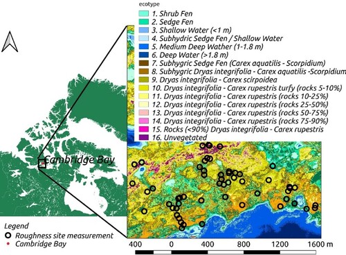
The ecotypes described in Figure 1 were determined using an ecosystem mapping approach (Ponomarenko et al. 2019) based on an ecosystem classification (McLennan et al. 2018). In total, 55 sites were used to create 3D point clouds for roughness measurements. These sites were classified in 4 different ecosystem types derived from the 15 classes displayed in Figure 1: (1) sedge/shrub, classes 1, 2 and 7; (2) organic soil (rock < 10%), classes 8, 9 and 10; (3) organic soil (rock < 75%), classes 11, 12 and 13; (4) rock > 75%, classes 14 and 15. It should be noted that for the sedge/shrub type, the roughness measurements were not of actual shrubs but rather of the area surrounding small vegetation.

3.2. Data

3.2.1. Roughness measurements

At each site, after sweeping the snow off without damaging the surface, approximately 30 downward facing photographs of the ground were taken using a standard compact camera (Canon Powershot Elph 160 5.0 mm). All sites were batch processed with Agisoft Metashape software using the same parameters for point cloud filtering (Normalized criterion for filtering: Reprojection error = 0.2, Reconstruction Uncertainty = 10.0, Projection Accuracy = 10.0), producing 3D models yielding approximately 2–4 million points each (Figure 2). Once a 3D point cloud is produced from 2D pictures, there is no scale to real world dimension. The relative distance between every point is accurate but lacks an absolute relationship. Known dimensions are then used to scale the 3D model. Using the software, we can define on the images the plate’s length so that these known dimensions can be used for optimization. Three metal plates of 50 cm each were used to scale the model where two were used for optimization of camera and position parameters and a third for validation yielding a precision of 0.1 mm by estimating the length of the third plates using optimization from first two plates. The plates need to be within as many pictures as possible without the radiometers field of view (FOV) becoming obstructed (after a radiometer measurement) so roughness can be measured. Light condition is also critical when doing photogrammetry, shadowing of half the surface could add uncertainty in reconstruction so constant illumination condition for every surface produced is desirable. Shadowing can be avoided while taking pictures by not going full circle around the sites, ¾ of a circle is sufficient for SfM to reconstruct the scene. This technique is fast and efficient in the field, producing reliable and precise measurements with only a standard digital camera and metal plates of known dimensions. These plates allow 3D models to be scaled without using a differential GPS unit with ground control points (GCP), e.g. Martinez-Agirre et al. (2019). The area covered for each 3D model ranged approximately from 0.25 to 0.6 ${\mathrm{m}}^2$. Dimensions can be seen for one site in Figure 2.

Figure 2. (a) 3D point cloud creation, (b) clipped 3D model to field of view of radiometer, (c) fitted plane to 3D surface and (d) histogram of perpendicular distances to plane, with ${\sigma }_H=1.3$ cm and 2,787,233 points.

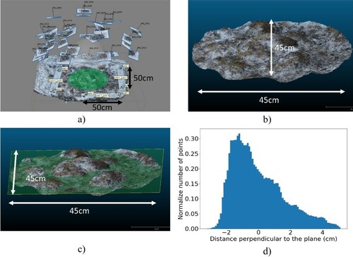
After the 3D reconstruction, the point cloud was clipped and a plane fitted by minimizing the mean perpendicular distance to zero. The height standard deviation was calculated with the perpendicular distance of every point to the plane and correlation length estimated using a variogram with x–y coordinates and height (z) from a randomly selected sub data set within point cloud (5000 points) where the fitted plane serves as the new x–y plane for the correlation in z. Several point clouds where tested (pairwise correlations calculations using up to 10,000 points) selected randomly from the entire point cloud. The correlation length converged on similar values irrespective of whether 5000 or 10,000 points were used. Therefore 5000 points was used for batch processing. Soil roughness is described at each site by the height standard deviation and correlation length. A fixed roughness parameter applicable to all sites was estimated with the mean of roughness parameters for all 55 sites. First the roughness value per site is used and then the mean roughness was tested for all simulations.

3.2.2. Radiometric data

Brightness temperatures were measured at all sites (April and May 2019) with surface-based radiometers (SBR) at 19 and 37 GHz mounted on a mobile sled measuring both vertical and horizontal polarizations. Snow was removed so as to measure only soil brightness temperature, and effective surface temperatures were recorded within the soil surface (2–3 cm) shielded from the sun using a probe thermometer with an accuracy of ±0.5°C at five different locations within the field of view of the radiometers. Among the 55 roughness sites analyzed, 21 radiometric measurements at 55° from nadir were recorded and calibrated using cold and warm targets (Asmus and Grant 1999) yielding an accuracy for radiometers of 2 K. Downward atmospheric contribution ($T_{B_{\mathrm{Atmo}\downarrow }}$) was estimated for each frequency using the amount of precipitable water in the 29 atmospheric layers from the North America Regional Reanalysis model (NARR) (Roy et al. 2012) within 32 × 32 km pixels. All sites are within the same pixel, thus variations in atmospheric contribution by date only represent changes in the atmosphere (see Table 2). Angular emissivity was also simulated ($e_H$ = 1–${\mathrm{\Gamma }}_H$ and $e_V$ = 1–${\mathrm{\Gamma }}_V$ derived from Equations (6) and (7)) using the Weg99 model (for incident angles between 0° and 60°) to analyze angular dependency. Using averaged measurements of soil temperature and atmospheric contribution of all sites, the mean measured emissivity at 55° (from Equations (1) and (2)) was calculated with standard variation (±0.009).

Table 2. Summary of radiometric observations and modeled downward atmospheric contributions.

Date	Number of sites	Mean Tsoil (°C)	Mean height std (cm)	Mean $T_B$ (K)				$T_B{}_{\mathrm{atmo}}\downarrow$ (K)
				19H	19V	37H	37V	19	37
2019-04-30	1	−17	1.6	235.5	239.8	240.4	244.4	12.5	25.5
2019-05-02	7	−14.1	1.4	244.6	251.2	247.7	252.3	13.5	26.1
2019-05-03	2	−14.8	2.1	242.8	252.1	247.6	253.0	11.7	24.9
2019-05-10	6	−10.1	2.4	248.5	249.4	250.1	252.4	14.9	27.1
2019-05-11	4	−9.6	1.9	254.2	256.1	256.4	258.2	15.5	27.5

Montpetit et al. (2018), hereafter noted Mont18, parametrized frozen sub-arctic tundra soil using multi-angular microwave observations. Based on Weg99 model retrieval, the Mont18 effective parameters shown in Table 3 are from a different site but can serve as a comparison in this study given that they were found from passive observations at 19 and 37 GHz such as conducted in our experiment. King et al. (2018) measured a permittivity of 4 + 0.5i also in a sub-Arctic environment in NWT, Canada. The retrieved permittivity values $({{\epsilon }^{\mathrm{\prime }}}_f-{{\epsilon }^{\mathrm{\prime }\mathrm{\prime }}}_{f}i)$ are in agreement with simulated permittivity using the soil radiative transfer model of Zhang et al. (2010) for frozen Arctic sites ($-{15}^{\circ }\mathrm{C}<T<-{10}^{\circ }\mathrm{C}$). The simulated values range from dry (wet) conditions: 3.13 − 0.0081i (4.63 − 0.0067i) and 3.11 − 0.0043i (4.61 − 0.0036i) respectively at 19 and 37 GHz (Table 3) with a sub-arctic soil composition (Clay = 9.66%, Sand = 50.73%, Silt = 39.61%). The values from Zhang et al. (2010) theoretical model (hereafter Zhang10) with a Volumetric Moisture Content (VMC) = 0.05 will be used as a reference value for the permittivity. The permittivity will then be optimized for all models to allow deviations from theoretical values to reflect the assumptions presented here.

Table 3. Parameters (Mont18) from optimization in Montpetit et al. (2018) with different soil moisture permittivity from model of Zhang et al. (2010).

Frequency (GHz)		$\epsilon$	${\beta }_f$	${\sigma }_H$ (cm)
Montpetit et al. (2018) optimization
19	Retrieved	3.42 − 0.005i	0.72	0.19
37		4.47 − 0.033i	0.42
Zhang et al. (2010) model
19	dry (VMC = 0.05)	3.13 − 0.008i
	wet (VMC = 0.6)	4.63 − 0.007i
37	dry (VMC = 0.05)	3.11 − 0.004i
	wet (VMC = 0.6)	4.61 − 0.004i

4. Results

4.1. Roughness measurements

Table 4 presents the results of all 55 sites, where both height standard deviation $({\sigma }_H)$and correlation length $(l_c)$were measured for each ecotype. The average ${\sigma }_H$ was 1.65 cm with $l_c$ of 39.5 cm.

Table 4. Mean value of roughness parameters measured with SfM photogrammetry.

Ecotype	Number of sites		Mean ${\sigma }_H$ (cm)	Std ${\sigma }_H$ (cm)	Mean $l_c$ (cm)	Std $l_c$ (cm)
	Roughness	Radiometric
Sedge/shrub	6	3	1.57	0.29	29.4	12.5
Organic soil (rock < 10%)	25	8	1.91	0.59	37.9	25.1
Organic soil (rock < 75%)	14	7	1.46	0.72	52.2	38.6
Rock > 75%	8	2	1.50	0.95	33.0	16.5
Total	55	20	1.65	0.71	39.5	28.3

Measured ${\sigma }_H$ greatly differs from Mont18 (${\sigma }_{\mathrm{eff}}$ = 0.19 cm), which was derived from a microwave optimization approach using Weg99. Effective roughness optimized in Mont18 using Weg99 yielded lower roughness values than the actual physical measurement. This point is examined in the discussion.

4.2. Brightness temperature simulation

Three soil emission models were tested using different roughness parameters and permittivity values as inputs in Equation (2). Model performances are shown in Figure 3 and summarized in Table 5. Simulated brightness temperatures from two semi-empirical models, QNH and Weg99, using dry permittivity from Zhang et al. (2010) model (${\epsilon }_{19}^{\mathrm{\prime }}$ = 3.13 and ${\epsilon }_{37}^{\mathrm{\prime }}$ = 3.11, Table 3) and roughness derived from SfM, were compared to SBR measurements (Figure 3(a,b)). The final model used was the Geo Optics (Figure 3(c)) analytical approach, which required two roughness parameters (${\sigma }_H$ and $l_c$) measured with SfM photogrammetry. Table 5 summarizes the root mean square errors (RMSE) and correlation (R²) between observed and simulated brightness temperatures shown in Figure 3 for all three models and parameters used. Results are first presented for all sites and for all sites without rocks (excluding two sites with rock > 75%), as they exhibit particular clusters. At rock-free sites: Sedge/shrub and Organic soil (rock < 10% and rock < 75%), Weg99 with ${\sigma }_H$ derived from SfM and permittivity from Zhang10 has one of the lowest RMSE with 3.3 K and highest R² of 0.71. RMSE for horizontal polarization (H pol) were generally higher than for V pol (high model dependency to the polarization ratio).

Figure 3. Simulations using Weg99, QNH and Geo optics models based on roughness estimates from SfM. Permittivity from Zhang10 was used. Polarization ratio (${\beta }_f$) used for Weg99 are (${\beta }_{f_{19}}=0.72$,${\beta }_{f_{37}}=0.42$) (Table 3) and parameters for QNH defined in Section 2.2.

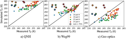
Table 5. Simulation results using roughness parameters from SfM and permittivity from Zhan10 model (dry: VMC = 0.05).

Model	Roughness	$\epsilon$	RMSE (K)
			19H	19V	37H	37V	Total	$R^2$
QNH	SfM	Zhang10	10.8	11.8	7.9	8.7	9.8	0.23
Weg99	SfM	Zhang10	7.3	7.4	5.5	4.9	6.3	0.13
Geo optics	SfM	Zhang10	9.2	9.3	10.1	7.9	9.1	0.07
No rock
QNH	SfM	Zhang10	8.2	8.0	5.9	6.9	7.2	0.68
Weg99	SfM	Zhang10	4.2	2.8	3.7	2.6	3.3	0.71
Geo optics	SfM	Zhang10	8.8	6.4	10.2	7.2	8.2	0.55

To investigate permittivity further and see if optimized values for every model would converge, each model using parameters from Table 5 without rock sites, were optimized from (1–10) for ${\epsilon }^{\mathrm{\prime }}$ and are shown in Figure 4 and Table 6. While QNH was optimized to lower RMSE, the value had no physical meaning since the permittivities are too high for frozen soil as optimization did not reach a minimum (${\epsilon }_{19}^{\mathrm{\prime }}$ = 10.0, ${\epsilon }_{37}^{\mathrm{\prime }}$ = 10.0). Weg99 and geo optics reached a minimum and indicating a low volumetric moisture content if we refer to Zhang et al. (2010) model values from Table 3. The Geo Optics model also shows a lower RMSE with 3.3 K when the permittivity is optimized (${\epsilon }_{19}^{\mathrm{\prime }}$ = 2.4, ${\epsilon }_{37}^{\mathrm{\prime }}$ = 2.3). The permittivity is outside Zhang et al. (2010) moisture interval presented in Table 3 however, there is uncertainty linked to the composition of soil type chosen.

Figure 4. Simulated vs measured brightness temperatures for all models with optimized permittivity in (a), (b), and (c) and optimization results in (d).

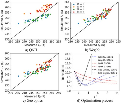
Table 6. Results from optimization of permittivity.

Model	${\epsilon }^{\mathrm{\prime }}$		RMSE (K)
	19	37	19H	19V	37H	37V	Total	$R^2$
QNH	10.0	10.0	4.3	6.0	3.1	5.0	4.6	0.51
Weg99	3.3	3.6	4.0	2.7	3.2	2.6	3.1	0.71
Geo optics	2.4	2.3	4.2	2.7	3.7	2.8	3.4	0.66

4.3. Analysis of rock sites

The two rocky sites (rock > 75%) had high biases in simulated brightness temperatures (Figure 3, and Table 5). It is difficult to precisely attribute the observed bias to only one factor (permittivity, temperature, structure of piled stones, see Figure 5(b)). Part of the deviation can result from the difference in permittivity between rocks and the mainly frozen organic soil at all the other sites. The ‘rocks’ found in the Greiner Watershed study site are in fact a loose part of a limestone bedrock emerging to the surface at the top of a hill (McLennan et al. 2018). The dielectric constant (${\epsilon }^{\mathrm{\prime }}$) of limestone was measured from 0.5 to 4.5 GHz in the recent study by Wang et al. (2020), giving values ranging from 8 to 8.5 at room temperature (∼20–25°C), and without trend within the range of frequency used. Even though this study is at higher frequencies and at lower temperatures (∼−10°C), this permittivity differs greatly from the Mont18 values used in this paper. Moreover, the five temperature measurements taken per site after snow removal and radiometric measurement yielded a mean temperature of −9.4 ± 1.4°C for both rock sites, while the mean rock temperature at the snow–rock interface was at −14°C and the air temperature was between −8 and −6°C during the experiments. Rock warming during the delay between the radiometric and temperature measurements might explain the observed difference in $T_B$ if we recall Equation (2), effective soil temperature is major component in $T_B$ calculation. Also, it is more difficult to measure rock temperature than organic soil with a probe thermometer. To investigate the potential impact of temperature differences, a sensitivity analysis was performed on the brightness temperature as a function of permittivity and temperature changes for the rock sites (Figure 5(a)).

Figure 5. (a) Representation of RMSE as function of permittivity and bias in effective temperature of the rock > 75% sites with Weg99 model and roughness SfM. (b) Image of one of the rock sites. (c) Simulation with modification of ϵ' = 8.3 and a change in temperature of $-8^{\circ }\mathrm{C}$ (from −9.4°C to −17°C) in Figure 5(a) for rock sites.

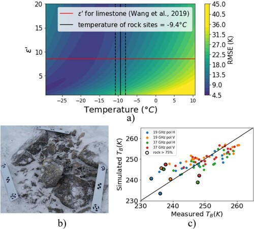
Figure 5(a) shows the RMSE associated with rock sites as a function of ${\epsilon }^{\mathrm{\prime }}$ and effective temperature compared to mean $T_B$ measurements at 19 and 37 GHz. Assuming ${\epsilon }^{\mathrm{\prime }}$ from Wang et al. (2020) (red line in Figure 5(a)), a low RMSE is reached with a change in temperature of $-8^{\circ }\mathrm{C}$ (from −9.4°C to −17°C in Figure 5(a)) from the measured temperature (black line). Soil temperature are presented in Table 2 with $T_{\mathrm{soil}}$ = −17°C for 2019-04-30, for which values are colder than air temperature given the fact that measurements occurred earlier during the Spring season. Figure 5(c) shows measured and simulated results when a fixed optimized temperature using Wang’s permittivity (8.3) is used for rock sites, giving a total RMSE of 3.8 K. Improvements are significant in the range of data uncertainties.

5. Sensitivity analysis and discussion

This discussion analyzes two points. We first examine the sensitivity of the considered soil emission model to the roughness variability at the 55 studied sites in the same tundra environment. Can a single value of roughness metrics be used to simulate emissivity of frozen arctic soil for global scale applications? We then discuss the observed differences between the measured physical roughness (by SfM) and the previously retrieved effective microwave roughness by Mont18.

We now explore the performance of a single roughness parameter applicable to all sites. The mean of roughness parameters was calculated for all 55 sites and then used as a reference value for all simulations (Table 7). Only Weg99 and Geo Optics models are presented as they had the lowest RMSE and highest R² values in Table 6. The mean value of ${\sigma }_H$ for Weg99 and the mean value of ${\sigma }_H$ and $l_c$ with $\epsilon$ = Table 6 were then applied as a fixed roughness metric in both models. Results in Table 7 show that the mean RMSE remains very similar to Table 5 and 6 (for Weg99, SfM, without rocks), suggesting that average roughness can be satisfactorily applied, despite the observed spatial variability (Table 4, 43% of variation coefficient). This offers confidence in using a single parameter for different sites (or roughness) as uncertainty due to local roughness variability may average out at larger scale.

Table 7. Summary of simulation with a fixed SfM value of roughness for all sites without rock.

		${\sigma }_H$ (cm)	$l_c$ (cm)	RMSE
				19H	19V	37H	37V	Total	$R^2$
Weg99	Mean	1.65		4.3	2.6	3.0	2.8	3.2	0.77
Geo Optics	Mean	1.65	39.5	4.2	2.7	3.9	2.7	3.4	0.71

The physical surface roughness measured by SfM differs greatly from the effective roughness parameter found at a different site by inverse modeling of 0.19 cm (Montpetit et al. 2018). This difference is consistent with conclusions from Tsang and Newton (1982) and Ulaby, Moore, and Fung (1982) that found discrepancy when using the QNH model. As such, the difference observed in our study when using Weg99 can also be attributed to the mix of QNH and the parametrization from Mo and Schmugge (1987). This explains the observed discrepancy between our measured roughness and the effective roughness found by Mont18.

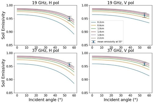
Also, in this study, all measurements were performed at 55° while multiple angles were used by Montpetit et al. (2018). The angular sensitivity of roughness is evaluated in Figure 6 for both frequencies and polarizations. All other factors being constant (soil moisture-permittivity in particular), roughness shows a stronger influence on emissivity at higher incidence angles (>50°), particularly for horizontal polarization. In other words, $e_p$ around and over 50° is more sensitive to roughness. This could be one of the reasons why multi-angular retrieved effective roughness does not match physically measured roughness (of the order of 2 cm, instead of 0.2 cm from Mont18). Other factors are also involved like the frequency dependency between 19 and 37 GHz. This greater sensitivity of emissivity at higher viewing angles was shown in the pioneering works of Wang et al. (1983) and Singh et al. (1995), which concluded that the best fit angle for satellite-borne surface roughness observations is near 50° for both polarizations.

Figure 6. Sensitivity analysis on angular dependency of emission with different roughness values, for 19 and 37 GHz with horizontal and vertical polarization.

Our results are also in agreement with results from King et al. (2018), who studied similar types of tundra environment. Using airborne dual band SAR radar measurements at 9.6 and 17.2 GHz, they found an optimized effective roughness of 1.3 cm at an incident angle of 40°.

Very few values of estimated effective roughness at high frequencies have been validated against in-situ roughness estimates. One reason is that previous techniques, such as those that use pin profilometers, are time consuming and best for point values, while modern techniques, such as laser scanning and SfM (Martinez-Agirre et al. 2019), are relatively easy to use and efficient for large-scale studies. Rahman et al. (2008) showed that the effective bare soil roughness at C-band (5.3 GHz) retrieved from radar measurements using the IEM model is of 2.19 ± 0.49 cm, while in-situ pin profilometer measurements gave a significantly lower soil roughness value of 0.79 ± 0.29 cm.

Our results also show permittivity values that are representative of spatial variability and permittivity fluctuations within studied soil types, as multiple landcovers were part of the in-situ validation. In the literature, in-situ permittivity values and roughness for frozen soils are currently rare, our study offers measured roughness values with permittivity and soil moisture that are valid with assumptions made within the Zhang et al. (2010) model. Results from this study could be generalized spatially, for example on a catchment scale, by linking in-situ results (roughness and permittivity) to the types of land cover. Increasingly, it is possible to derive centimeter scale roughness information from UAVs that characterize different hydrological response units within catchments. In addition, topographic and ecological land-cover classes can be derived from very high-resolution optical satellite images (such as WORLDVIEW-3 images), which opens opportunities for application of roughness to land cover classes over larger pan-Arctic scales.

6. Conclusion

In this study, we applied an effective and relatively simple method to measure soil roughness at multiple Arctic sites using the Structure-from-Motion (SfM) technique. Measurements of surface roughness over 55 sites across 4 Arctic tundra ecotypes had an average RMS height (${\sigma }_H$) of 1.65 cm and mean 2 $D_{x,y}$ correlation length ($l_c$) of 39.5 cm. The observed variability appears relatively low for ${\sigma }_H$ but high for $l_c$. For the first time, we tested three different rough surface reflectivity models (QNH, Weg99 and Geo Optics) at 19 and 37 GHz over frozen ground conditions and compared simulations to ground-based radiometer observations. Results show best performance with the Weg99 model parametrized with SfM-based roughness (1.65 cm) and frozen organic soil permittivity $(\epsilon )$ from theoretical model by Zhang et al. (2010). When permittivity is optimized, Weg99 still best fit observations. Accuracy considering fixed permittivity and measured roughness at each site for Tb simulations yielded similar results indicating a fixed value could be used for large scale application. The Geo Optics model also shows good results if the permittivity is optimized (see Table 6).

A fixed value for roughness (${\sigma }_H$) for all the sites gives similar modeling performance even though variability of ${\sigma }_H$ between sites was observed. The mean roughness value of ${\sigma }_H=1.65\mathrm{cm}$ and $\epsilon$given in Table 6 using the Weg99 model appears to be representative of Arctic tundra land cover, mainly characterized by sedge/shrub with organic soil and rock between 10% and 75%.

Analysis of particular rock sites with limestone composition and similar roughness to organic soils revealed different behavior in radiometric measurements, suggesting a need to consider specific rock permittivity and a colder effective temperature to match simulations and observations. This is an important finding as rock surfaces cover up to 8% of terrestrial high Arctic areas (Ponomarenko et al. 2019). Because of the large difference in permittivity between rocks and soil, future studies may consider a mixed model that takes into account the fraction of rocks in each land cover or geological class. This could be useful in inversion of parameters for remote sensing planetary surfaces.

This study thus offers surface roughness values that can be used on a larger scale in a satellite retrieval algorithm for global Arctic monitoring by remote sensing. Using inversion algorithm to retrieve surface parameters is difficult because both backscattering coefficient and brightness temperature are strongly affected in the same way by several factors including roughness, soil moisture, vegetation or snow cover (e.g. Moradizadeh and Saradjian 2016; Wigneron et al. 2017). The reduction in microwave dielectric sensitivity to soil moisture caused by surface roughness is a well-known problem. In addition, estimating these parameters remains challenging, as shown in numerous studies (e.g. Du, Shi, and Sun 2010, with active radiometry; Roy et al. 2016; Shi, Xiong, and Jiang 2016, with passive radiometry). For example, surface roughness change linked to land cover change, such as observed shrub expansion in the Arctic, could be an important source of uncertainties for modeling active and passive microwave signals. The photogrammetry method presented in this paper offers an effective and low-cost way to reliably measure soil roughness when performing ground-based validation of passive/active microwave data while allowing us to gain a better understanding of geophysical properties of frozen soil.

Acknowledgements

The authors would like to thank Benoît Montpetit and Alex Mavrovic for their contribution and helpful comments on this work. We thank Donald McLennan, Johann Wagner and Serguei Ponomarenko for the ecosystem map and their help in Cambridge Bay. We also thank Daniel Kramer, Simon Levasseur, Coralie Gautier, Guillaume Couture and Patrick Cliche from Université de Sherbrooke and Ludovic Brucker from the NASA Cryospheric Sciences Laboratory for field work assistance, instrument maintenance and overall guidance.

Data availability statement

All brightness temperatures and emissivity values will be available on request.

Disclosure statement

No potential conflict of interest was reported by the author(s).

Additional information

Funding

This research was made possible thanks to the financial support of the Natural Sciences and Engineering Research Council of Canada (NSERC), Polar Knowledge Canada, Canada Foundation for Innovation (CFI), Fonds québécois de la recherche sur la nature et les technologies (FRQNT-Québec), Northern Scientific Training Program (NSTP), Environment and Climate Change Canada Grant and Contribution program and research funding from Northumbria University, UK.

Notes

Note: Permittivity from Montpetit et al. (2018) was used for calculation.

Note: VMC stands for volumetric moisture content.

References

- Asmus, K. W., and C. Grant. 1999. “Surface Based Radiometer (SBR) Data Acquisition System.” International Journal of Remote Sensing 20 (15–16): 3125–3129. doi:https://doi.org/10.1080/014311699211651.
- Bühler, Yves, Marc S. Adams, Andreas Stoffel, and Ruedi Boesch. 2017. “Photogrammetric Reconstruction of Homogenous Snow Surfaces in Alpine Terrain Applying Near-Infrared UAS Imagery.” International Journal of Remote Sensing 38 (8–10): 3135–3158. doi:https://doi.org/10.1080/01431161.2016.1275060.
- Chen, K. S., Tzong-Dar Wu, Leung Tsang, Qin Li, Jiancheng Shi, and A.K. Fung. 2003. “Emission of Rough Surfaces Calculated by the Integral Equation Method with Comparison to Three-Dimensional Moment Method Simulations.” IEEE Transactions on Geoscience and Remote Sensing. doi:10.1109.TGRS.2002.807587.
- Choudhury, B. J., T. J. Schmugge, A. Chang, and R. W. Newton. 1979. “Effect of Surface Roughness on the Microwave Emission from Soils.” Journal of Geophysical Research 84 (C9): 5699. doi:https://doi.org/10.1029/JC084iC09p05699.
- Derksen, C., J. Lemmetyinen, P. Toose, A. Silis, J. Pulliainen, and M. Sturm. 2014. “Physical Properties of Arctic Versus Subarctic Snow: Implications for High Latitude Passive Microwave Snow Water Equivalent Retrievals.” Journal of Geophysical Research: Atmospheres 119 (12): 7254–7270. doi:https://doi.org/10.1002/2013JD021264.
- Dobson, Myron, Fawwaz Ulaby, Martti Hallikainen, and Mohamed El-rayes. 1985. “Microwave Dielectric Behavior of Wet Soil-Part II: Dielectric Mixing Models.” IEEE Transactions on Geoscience and Remote Sensing GE-23 (1): 35–46. doi:https://doi.org/10.1109/TGRS.1985.289498.
- Du, Jinyang, Jiancheng Shi, and Ruijing Sun. 2010. “The Development of HJ SAR Soil Moisture Retrieval Algorithm.” International Journal of Remote Sensing 31 (14): 3691–3705. doi:https://doi.org/10.1080/01431161.2010.483486.
- Fung, A.K. 1994. Microwave Scattering and Emission Models and Their Applications. Boston: Artech House Publishers.
- Gharechelou, Saeid, Ryutaro Tateishi, and Brian A. Johnson. 2018. “A Simple Method for the Parameterization of Surface Roughness from Microwave Remote Sensing.” Remote Sensing 10 (11): 1711. doi:https://doi.org/10.3390/rs10111711.
- King, Joshua, Chris Derksen, Peter Toose, Alexandre Langlois, Chris Larsen, Juha Lemmetyinen, Phil Marsh, et al. 2018. “The Influence of Snow Microstructure on Dual-Frequency Radar Measurements in a Tundra Environment.” Remote Sensing of Environment 215 (May): 242–254. doi:https://doi.org/10.1016/j.rse.2018.05.028.
- Kong, Jin Au, and Leung Tsang. 2001. Scattering of Electromagnetic Waves. Vol. 3. New York: Wiley.
- Lawrence, Heather, François Demontoux, Jean-Pierre Wigneron, Philippe Paillou, Tzong-Dar Wu, and Yann H. Kerr. 2011. “Evaluation of a Numerical Modeling Approach Based on the Finite-Element Method for Calculating the Rough Surface Scattering and Emission of a Soil Layer.” IEEE Geoscience and Remote Sensing Letters 8 (5): 953–957. doi:https://doi.org/10.1109/LGRS.2011.2131633.
- Lawrence, Heather, Jean-Pierre Wigneron, Francois Demontoux, Arnaud Mialon, and Yann H. Kerr. 2013. “Evaluating the Semiempirical H-Q Model Used to Calculate the L-Band Emissivity of a Rough Bare Soil.” IEEE Transactions on Geoscience and Remote Sensing 51 (7): 4075–4084. doi:https://doi.org/10.1109/TGRS.2012.2226995.
- Lejot, J., C. Delacourt, H. Piégay, T. Fournier, M.-L. Trémélo, and P. Allemand. 2007. “Very High Spatial Resolution Imagery for Channel Bathymetry and Topography from an Unmanned Mapping Controlled Platform.” Earth Surface Processes and Landforms 32 (11): 1705–1725. doi:https://doi.org/10.1002/esp.1595.
- Martinez-Agirre, Alex, Jesús Álvarez-Mozos, Milutin Milenković, Norbert Pfeifer, Rafael Giménez, José Manuel Valle Melón, and Álvaro Rodríguez Miranda. 2019. “Evaluation of Terrestrial Laser Scanner and Structure from Motion Photogrammetry Techniques for Quantifying Soil Surface Roughness Parameters over Agricultural Soils.” Earth Surface Processes and Landforms, esp.4758. doi:https://doi.org/10.1002/esp.4758.
- McLennan, Donald S., William H. MacKenzie, Del Meidinger, Johann Wagner, and Christopher Arko. 2018. “A Standardized Ecosystem Classification for the Coordination and Design of Long-Term Terrestrial Ecosystem Monitoring in Arctic-Subarctic Biomes.” Arctic 71 (5): 1–15. doi:https://doi.org/10.14430/arctic4621.
- Mironov, Valery L., Liudmila G. Kosolapova, Yury I. Lukin, Andrey Y. Karavaysky, and Illia P. Molostov. 2017. “Temperature- and Texture-Dependent Dielectric Model for Frozen and Thawed Mineral Soils at a Frequency of 1.4 GHz.” Remote Sensing of Environment 200 (August): 240–249. doi:https://doi.org/10.1016/j.rse.2017.08.007.
- Mo, Tsan, and Thomas J. Schmugge. 1987. “A Parameterization of the Effect of Surface Roughness on Microwave Emission.” IEEE Transactions on Geoscience and Remote Sensing GE-25 (4): 481–486. doi:https://doi.org/10.1109/TGRS.1987.289860.
- Mo, Tsan, Thomas J. Schmugge, and James R. Wang. 1987. “Calculations of the Microwave Brightness Temperature of Rough Soil Surfaces: Bare Field.” IEEE Transactions on Geoscience and Remote Sensing GE-25 (1): 47–54. doi:https://doi.org/10.1109/TGRS.1987.289780.
- Montpetit, B., A. Royer, A. Roy, and A. Langlois. 2018. “In-Situ Passive Microwave Emission Model Parameterization of Sub-Arctic Frozen Organic Soils.” Remote Sensing of Environment 205 (November 2017): 112–118. doi:https://doi.org/10.1016/j.rse.2017.10.033.
- Montpetit, B., A. Royer, J. P. Wigneron, A. Chanzy, and A. Mialon. 2015. “Evaluation of Multi-Frequency Bare Soil Microwave Reflectivity Models.” Remote Sensing of Environment 162: 186–195. doi:https://doi.org/10.1016/j.rse.2015.02.015.
- Moradizadeh, Mina, and Mohammad R. Saradjian. 2016. “The Effect of Roughness in Simultaneously Retrieval of Land Surface Parameters.” Physics and Chemistry of the Earth, Parts A/B/C 94 (August): 127–135. doi:https://doi.org/10.1016/j.pce.2016.03.006.
- Murtiyoso, A., M. Koehl, P. Grussenmeyer, and T. Freville. 2017. “Acquisition and Processing Protocols for UAV Images: 3D Modeling of Historical Building Using Photogrammetry.” ISPRS Annals of Photogrammetry, Remote Sensing and Spatial Information Sciences IV-2/W2 (2W2): 163–170. doi:https://doi.org/10.5194/isprs-annals-IV-2-W2-163-2017.
- Njoku, E. G., T. J. Jackson, Venkataraman Lakshmi, T. K. Chan, and S. V. Nghiem. 2003. “Soil Moisture Retrieval from AMSR-E.” IEEE Transactions on Geoscience and Remote Sensing 41 (2): 215–229. doi:https://doi.org/10.1109/TGRS.2002.808243.
- Nolan, M., C. Larsen, and M. Sturm. 2015. “Mapping Snow Depth from Manned Aircraft on Landscape Scales at Centimeter Resolution Using Structure-from-Motion Photogrammetry.” Cryosphere 9 (4): 1445–1463. doi:https://doi.org/10.5194/tc-9-1445-2015.
- Picard, G., L. Brucker, A. Roy, F. Dupont, M. Fily, A. Royer, and C. Harlow. 2013. “Simulation of the Microwave Emission of Multi-Layered Snowpacks Using the Dense Media Radiative Transfer Theory: The DMRT-ML Model.” Geoscientific Model Development 6 (4): 1061–1078. doi:https://doi.org/10.5194/gmd-6-1061-2013.
- Picard, Ghislain, Melody Sandells, and Henning Löwe. 2018. “SMRT: An Active-Passive Microwave Radiative Transfer Model for Snow with Multiple Microstructure and Scattering Formulations (v1.0).” Geoscientific Model Development 11 (7): 2763–2788. doi:https://doi.org/10.5194/gmd-11-2763-2018.
- Ponomarenko, Serguei, Donald McLennan, Darren Pouliot, and Johann Wagner. 2019. “High Resolution Mapping of Tundra Ecosystems on Victoria Island, Nunavut – Application of a Standardized Terrestrial Ecosystem Classification.” Canadian Journal of Remote Sensing 45 (5): 551–571. doi:https://doi.org/10.1080/07038992.2019.1682980.
- Rahman, M. M., M. S. Moran, D. P. Thoma, R. Bryant, C. D. Holifield Collins, T. Jackson, B. J. Orr, and M. Tischler. 2008. “Mapping Surface Roughness and Soil Moisture Using Multi-Angle Radar Imagery Without Ancillary Data.” Remote Sensing of Environment 112 (2): 391–402. doi:https://doi.org/10.1016/j.rse.2006.10.026.
- Roy, Alexandre, Ghislain Picard, Alain Royer, Benoit Montpetit, Florent Dupont, Alexandre Langlois, Chris Derksen, and Nicolas Champollion. 2013. “Brightness Temperature Simulations of the Canadian Seasonal Snowpack Driven by Measurements of the Snow Specific Surface Area.” IEEE Transactions on Geoscience and Remote Sensing 51 (9): 4692–4704. doi:https://doi.org/10.1109/TGRS.2012.2235842.
- Roy, Alexandre, Alain Royer, Olivier St-Jean-Rondeau, Benoit Montpetit, Ghislain Picard, Alex Mavrovic, Nicolas Marchand, and Alexandre Langlois. 2016. “Microwave Snow Emission Modeling Uncertainties in Boreal and Subarctic Environments.” The Cryosphere 10 (2): 623–638. doi:https://doi.org/10.5194/tc-10-623-2016.
- Roy, Alexandre, Alain Royer, Jean-Pierre Wigneron, Alexandre Langlois, Jean Bergeron, and Patrick Cliche. 2012. “A Simple Parameterization for a Boreal Forest Radiative Transfer Model at Microwave Frequencies.” Remote Sensing of Environment 124 (September): 371–383. doi:https://doi.org/10.1016/j.rse.2012.05.020.
- Royer, Alain, Alexandre Roy, Benoit Montpetit, Olivier Saint-Jean-Rondeau, Ghislain Picard, Ludovic Brucker, and Alexandre Langlois. 2017. “Comparison of Commonly-Used Microwave Radiative Transfer Models for Snow Remote Sensing.” Remote Sensing of Environment 190 (November): 247–259. doi:https://doi.org/10.1016/j.rse.2016.12.020.
- Saberi, Nastaran, Richard Kelly, Margot Flemming, and Qinghuan Li. 2020. “Review of Snow Water Equivalent Retrieval Methods Using Spaceborne Passive Microwave Radiometry.” International Journal of Remote Sensing 41 (3): 996–1018. doi:https://doi.org/10.1080/01431161.2019.1654144.
- Shi, JianCheng, Chuan Xiong, and LingMei Jiang. 2016. “Review of Snow Water Equivalent Microwave Remote Sensing.” Science China Earth Sciences 59 (4): 731–745. doi:https://doi.org/10.1007/s11430-015-5225-0.
- Singh, K. P., D. Singh, S. K. Sharma, and P. K. Mukherjee. 1995. “Remote Sensing of Earth’s Surface Roughness at Microwave Frequency.” Advances in Space Research 16 (10): 189–192. doi:https://doi.org/10.1016/0273-1177(95)00402-Z.
- Snapir, B., S. Hobbs, and T. W. Waine. 2014. “Roughness Measurements over an Agricultural Soil Surface with Structure from Motion.” ISPRS Journal of Photogrammetry and Remote Sensing 96 (October): 210–223. doi:https://doi.org/10.1016/j.isprsjprs.2014.07.010.
- Trudel, Mélanie, François Charbonneau, Fernando Avendano, and Robert Leconte. 2010. “Quick Profiler (QuiP): A Friendly Tool to Extract Roughness Statistical Parameters Using a Needle Profiler.” Canadian Journal of Remote Sensing 36 (4): 391–396. doi:https://doi.org/10.5589/m10-070.
- Tsang, Leung, Kung Hau Ding, Shaowu Huang, and Xiaolan Xu. 2013. “Electromagnetic Computation in Scattering of Electromagnetic Waves by Random Rough Surface and Dense Media in Microwave Remote Sensing of Land Surfaces.” Proceedings of the IEEE 101 (2): 255–279. doi:https://doi.org/10.1109/JPROC.2012.2214011.
- Tsang, Leung, Jin Au Kong, and Kung Hau Ding. 2000. Scattering of Electromagnetic Waves. Vol. 1. New York: Wiley. doi:https://doi.org/10.1201/9780429431210-3.
- Tsang, Leung, Tien Hao Liao, Shurun Tan, Huanting Huang, Tai Qiao, and Kung Hau Ding. 2017. “Rough Surface and Volume Scattering of Soil Surfaces, Ocean Surfaces, Snow, and Vegetation Based on Numerical Maxwell Model of 3-D Simulations.” IEEE Journal of Selected Topics in Applied Earth Observations and Remote Sensing 10 (11): 4703–4720. doi:https://doi.org/10.1109/JSTARS.2017.2722983.
- Tsang, L., and R. W. Newton. 1982. “Microwave Emissions from Soils with Rough Surfaces.” Journal of Geophysical Research 87 (C11): 9017–9024. doi:https://doi.org/10.1029/JC087iC11p09017.
- Turner, Russell, Rocco Panciera, Mihai A. Tanase, Kim Lowell, Jorg M. Hacker, and Jeffrey P. Walker. 2014. “Estimation of Soil Surface Roughness of Agricultural Soils Using Airborne LiDAR.” Remote Sensing of Environment 140: 107–117. doi:https://doi.org/10.1016/j.rse.2013.08.030.
- Ulaby, F. T., R. K. Moore, and A. K. Fung. 1982. Microwave Remote Sensing: Active and Passive. Volume II. Radar Remote Sensing and Surface Scattering and Emission Theory. Boston: Addison-Wesley.
- Wang, J. R., and B. J. Choudhury. 1981. “Remote Sensing of Soil Moisture Content over Bare Field at 1.4 GHz Frequency.” Journal of Geophysical Research 86 (C6): 5277–5282. doi:https://doi.org/10.1029/JC086iC06p05277.
- Wang, James R., Peggy E. O’Neill, Thomas J. Jackson, and Edwin T. Engman. 1983. “Multifrequency Measurements of the Effects of Soil Moisture, Soil Texture, and Surface Roughness.” IEEE Transactions on Geoscience and Remote Sensing GE-21 (1): 44–51. doi:https://doi.org/10.1109/TGRS.1983.350529.
- Wang, Shaofei, Qiang Sun, Nianqin Wang, and Lei Yang. 2020. “Variation in the Dielectric Constant of Limestone with Temperature.” Bulletin of Engineering Geology and the Environment 79 (3): 1349–1355. doi:https://doi.org/10.1007/s10064-019-01647-3.
- Wegmüller, Urs, and Christian Mätzler. 1999. “Rough Bare Soil Reflectivity Model.” IEEE Transactions on Geoscience and Remote Sensing 37 (3 I): 1391–1395. doi:https://doi.org/10.1109/36.763303.
- Westoby, M. J., J. Brasington, N. F. Glasser, M. J. Hambrey, and J. M. Reynolds. 2012. “‘Structure-from-Motion’ Photogrammetry: A Low-Cost, Effective Tool for Geoscience Applications.” Geomorphology 179: 300–314. doi:https://doi.org/10.1016/j.geomorph.2012.08.021.
- Wigneron, J. P., T. J. Jackson, P. O’Neill, G. De Lannoy, P. de Rosnay, J. P. Walker, P. Ferrazzoli, et al. 2017. “Modelling the Passive Microwave Signature from Land Surfaces: A Review of Recent Results and Application to the L-Band SMOS & SMAP Soil Moisture Retrieval Algorithms.” Remote Sensing of Environment 192 (January): 238–262. doi:https://doi.org/10.1016/j.rse.2017.01.024.
- Wigneron, J.-P., Laurent Laguerre, and Y. H. Kerr. 2001. “A Simple Parameterization of the L-Band Microwave Emission from Rough Agricultural Soils.” IEEE Transactions on Geoscience and Remote Sensing 39 (8): 1697–1707. doi:https://doi.org/10.1109/36.942548.
- Zhang, Lixin, Jiancheng Shi, Zhongjun Zhang, and Kaiguang Zhao. 2003. “The Estimation of Dielectric Constant of Frozen Soil-Water Mixture at Microwave Bands.” International Geoscience and Remote Sensing Symposium 4 (40271080): 2903–2905. doi:https://doi.org/10.1109/igarss.2003.1294626.
- Zhang, Lixin, Tianjie Zhao, Lingmei Jiang, and Shaojie Zhao. 2010. “Estimate of Phase Transition Water Content in Freeze-Thaw Process Using Microwave Radiometer.” IEEE Transactions on Geoscience and Remote Sensing 48 (12): 4248–4255. doi:https://doi.org/10.1109/TGRS.2010.2051158.
- Zheng, Xingming, Zhao Kai, Li Xiaojie, Li Yangyang, and Ren Jianhua. 2014. “Improvements in Farmland Surface Roughness Measurement by Employing a New Laser Scanner.” Soil and Tillage Research 143 (November): 137–144. doi:https://doi.org/10.1016/j.still.2014.06.010.