Chlorophyll-a concentrations in 82 large alpine lakes on the Tibetan Plateau during 2003–2017: temporal–spatial variations and influencing factors

ABSTRACT

As essential parts of the unique ecosystem of Tibetan Plateau (TP), the sizes and associated physical properties of alpine lakes have long been investigated. However, little is known about one of the most critical biogeochemical properties, i.e. the Chlorophyll-a (Chl-a) concentrations. Here, for the first time, we presented a comprehensive investigation of the temporal–spatial variations in Chl-a in 82 lakes (>50 km²) across the entire TP region, based on MODIS observations in the period of 2003–2017. The results showed that the 82 lakes exhibited an average long-term mean Chl-a of 3.3  ±  4.3 mg m⁻³, with high Chl-a lakes concentrated in the eastern and southern inner TP basin and northeastern parts of the TP. An interannual trend analysis revealed that lakes exhibiting (significantly) decreasing Chl-a trends and (significantly) increasing Chl-a trends were comparable in numbers but differed in distribution patterns. A correlation analysis indicated that at least 70% of the interannual variability in Chl-a values of lakes was significantly correlated with one of the four environmental factors (wind speed, ice cover duration, lake water surface temperature and surface runoff) and lake size. In addition, glacier meltwater tended to reduce lake Chl-a while salinity levels showed minor influences.

KEYWORDS:

• Chlorophyll-a
• inland water
• Tibetan Plateau
• remote sensing
• alpine lake

1. Introduction

The Tibetan Plateau (TP), which is widely regarded as the Asian Water Tower, is the cradle of many large international rivers and serves as an indispensable part of the water supply for many countries across Asia. Due to the harsh and unique natural conditions, the TP is minimally disturbed by human activities but is very sensitive to climate changes characterized by significant warming and varied changes in other important climate factors, such as precipitation, evapotranspiration, wind and sunshine duration (Qiu 2008; Kuang and Jiao 2016b). The dense distribution of alpine water bodies, combined with widespread glaciers and permafrost in the TP region, make the region a unique ecosystem. Lakes in the TP are profoundly affected by regional climate change (Zhang et al. 2017b), which could in turn exert a significant impact on the regional climate through biophysical feedbacks. Therefore, the dynamics of lakes in the TP have drawn widespread attention from society and scholars (Lei and Yang 2017).

A series of studies have focused on lake physical properties in the TP region, including lake area (Song et al. 2014c; Zhang et al. 2017b; Sun et al. 2018a), lake level (Song et al. 2014a; Jiang et al. 2017), lake water storage (Zhang et al. 2017c; Qiao, Zhu, and Yang 2019b), lake ice phenology (Guo et al. 2018; Cai et al. 2019), lake surface water temperature (Zhang et al. 2014a; Wan et al. 2017a) and so on. However, little attention has been given to the biogeochemical properties of lakes in the TP, such as chlorophyll-a (Chl-a) concentration. Chl-a is a key indicator of eutrophication status and water's primary productivity and is therefore essential for understanding related biogeochemical processes in lakes (Guildford and Hecky 2000; Gons, Auer, and Effler 2008; Hu, Lee, and Franz 2012; Lyche-Solheim et al. 2013). Detailed documentation of spatial and temporal Chl-a distribution in the TP would greatly benefit regional water resource management, environmental regulation and relevant research (Sayers et al. 2015).

Owing to the extreme environment (altitude above 4000 m), the majority of lakes in the TP are located in the depopulated zone, characterized by low accessibility of traffic networks and shortages of vessels for cruise surveys. Regular in situ sampling or field monitoring of Chl-a for the myriad lakes across the entire TP region is therefore hampered by its inherent constraints in spatiotemporal coverage as well as the inconvenience and high cost resulting from the extreme environments. As a feasible alternative, remote sensing has shown great potential in providing large-scale and continuous time series of Chl-a observations across various spatial and temporal domains. Currently, numerous ocean color satellite sensors have been widely applied in deriving Chl-a distributions, including the Sea-Viewing Wide Field-of-View Sensor (SeaWiFS), the Moderate Resolution Imaging Spectroradiometer (MODIS), the Visible Infrared Imaging Radiometer Suite (VIIRS), the Medium Resolution Spectroradiometer (MERIS) and its successor, the Sentinel-3 Ocean and Land Color Instrument (OLCI). It is undeniable that relevant research using these satellite observations facilitates a deeper understanding of the variations in the geochemical and biochemical properties of water bodies to a certain extent (Behrenfeld and Boss 2006; McClain 2009). However, there is no such a study focusing on a comprehensive assessment of the spatial–temporal Chl-a distribution over the unique region of the TP, which is critical for its function as the Asian Water Tower.

Lakes in the TP have witnessed dramatic changes during the past few decades. For instance, Zhang et al. studied the lakes larger than 1 km² across the TP and observed a 31.9%'s growth in the lake number (from 1080 to 1424) and an increase of 25.4% in the lake surface area (from ∼ 4.0 × 104 to ∼ 5.0 × 104 km²) during the period of 1970s to 2018 (Zhang et al. 2014b; Zhang et al. 2019b). The same phenomena have been found in many other studies, and further indicated the linkage of rapid lake expansion in the TP (especially in the central TP) with the accelerated shrinkage of glaciers since 1990 (Lei et al. 2014; Song et al. 2014c; Yang et al. 2017; Zhang et al. 2017b). In the southern part of the TP, opposite changes have been observed (Zhang et al. 2011, 2013). Associated with these observed changes, it is interesting to further explore the potential impacts of lake size on Chl-a concentration in general. In fact, the influence of lake size variations on Chl-a is rather complex. The dynamics of lake size are a combined result of direct impacts from different climate factors such as air temperature, evaporation, precipitation, and climate-induced glacial melt (Song et al. 2014b; Zhang et al. 2017a; Sun et al. 2018b; Qiao, Zhu, and Yang 2019a). Each of these particular factors can have different magnitudes of impact on the changes in lake size and can further trigger other processes to impact lake Chl-a. Taking glacier meltwater as an example, as an essential contributor to lake expansion, the meltwater-associated decrease in water temperature and increase in light attenuation were found to modulate phytoplankton growth and thus impact lake Chl-a concentrations (Vinebrooke et al. 2010; Rose et al. 2014).

To fill the knowledge gaps in the Chl-a variations and their potential impact factors, the current study was designed to (1) present a first comprehensive glance of the variation in lake Chl-a at both spatial and temporal scales in the TP region using long-term Chl-a products from MODIS Aqua between 2003 and 2017 and to (2) explore the potential impacts of lake size variations and several other key environmental factors on lake Chl-a. To achieve these objectives, the paper is structured as follows. In the first step, the data and methods adopted in this study are introduced, including the background of the study area, procedures for satellite-based Chl-a retrieval along with the selection principles and data sources of relevant environmental driving factors. Then, a detailed description of the interannual and monthly changes in Chl-a is presented. In the next step, the potential effects of lake size, wind speed, lake surface water temperature (LSWT), ice cover duration (ICD), surface runoff, glaciers and salinity are investigated, which is followed by a brief discussion on other potential factors that are not statistically explored. Finally, the uncertainty, validity and future implications of satellite-derived Chl-a in the TP region are discussed.

2. Materials and methods

2.1. Study area

Our study area, the TP, is located in the western part of China and central Asia, within latitudes 26°00′N-39°47′N and longitudes 73°19′E-104°47′E. The TP is recognized as ‘the roof of the world’, as its mean elevation is over 4000 m above sea level. The TP's profound spatial variations in climate is governed by the Asian monsoon system and the westerlies (Krause et al. 2010; Yao et al. 2012), resulting in a relatively warm and humid climate conditions in the southeastern part of TP and a cold and arid climate in the northwestern TP (Yin et al. 2013). The entire TP region covers approximately 2.5 × 10⁶ km², and thousands of lakes can be identified (Kuang and Jiao 2016a). Among those lakes, approximately 1400 lakes are larger than 1 km²in 2018 (Zhang et al. 2019a).

The majority of lakes on TP belong to salt or salt water lakes, especially those endorheic lakes distributed at the inner TP basin (Lin et al. 2020). The hydrochemistry condition of TP's alpine lake system were reported to be influenced by many geological and climatic factors, including atmospheric precipitation, glacial meltwater, rock weathering and evapo-crystallization processes and is also intervened by human activities (Pant et al. 2018; Yang et al. 2019). Like many other high altitude lakes, the lakes on TP are generally characterized by low biodiversity and simple ecosystem structure (Kong et al. 2017; Ren et al. 2017). In addition, a broad satellite observation on the water clarity changes of 64 large alpine lakes also indicated that the lakes on TP are relatively clear (especially those in the southern and northeastern TP), with a long-term mean Z_sd of 4.4 m (Pi et al. 2020).

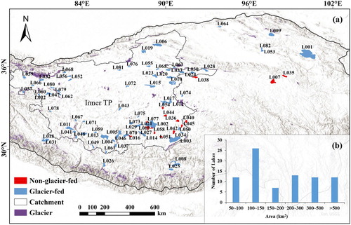
For the current Chl-a analysis, 82 lakes were selected based on the image quality (i.e. relatively lesser cloud cover and less missing Chl-a values on satellite retrievals) and lake size (larger than 50 km²). Among these selected lakes, Qinghai Lake (4232 km²) and Keluke Lake (54 km²) are the largest lake and smallest lake, respectively. Together, they account for around 65% of the total lake area of the TP. Detailed information about the selected lakes is presented in Table A1. The distribution of those lakes as well as whether they are glacier-fed lakes is presented in Figure 1a (Wang and Dou 1998), along with the percentage of lakes that fall into each size group (50–100 km², >500 km², and so on) is shown in Figure 1b.

Figure 1. (a) Locations of the 82 examined lakes on the TP. Lakes annotated with red colors receive water from glacial melt, while lakes marked by blue colors do not. (b) The histogram shows the number of lakes characterized by size.

2.2. Satellite-derived Chl-a concentrations

Level-2 ocean color images from MODIS Aqua, MODSI Terra and VIIRS were obtained from the NASA Ocean Color Web Archive (https://oceancolor.gsfc.nasa.gov/). MODIS Aqua data were used to examine the Chl-a trends for the TP lakes, and Chl-a estimates from both MODIS Terra and VIIRS were used to partially evaluate the fidelity of the derived trends from Aqua. All level-2 files from MODIS Aqua and Terra in the 2003–2017 period were downloaded, while data from VIIRS were not available until 2012. The numbers of images available for MODIS Aqua, MODIS Terra and VIIRS are 14,447, 15,188 and 6091, respectively. Note that the data between June and October during each year was used because many lakes were covered by ice during the other months. The 1-km-resolution data were kept with the same cylindrical equidistance projection through the SeaDAS software (version 7.5). Quality control flags were applied for the images to reduce the potential errors caused by unfavorable observation conditions (i.e. clouds and straylight in this study), and data that failed to satisfy the quality control criterion of NASA (https://oceancolor.gsfc.nasa.gov/atbd/ocl2flags/) were discarded. Note that a 3 × 3 pixel straylight mask was conducted in replacement of the default 7 × 5 pixel window to improve data coverage for these lakes, as such a process has demonstrated limited impacts on data quality (Hu et al. 2019).

The Chl-a concentrations in each level 2 file were the default Chl-a product, which is estimated with the combination of the color index-based (CI-based) algorithm (Hu, Lee, and Franz 2012) for Chl-a poor waters (with Chl-a values <0.15 mg m⁻³) and the blue-to-green band ratio algorithm (OCx-based) for Chl-a rich waters (O’Reilly et al. 1998). For lakes in the TP, the OCx algorithm is apparently more applicable because the Chl-a values are expected to be higher than 0.3 mg m⁻³, as demonstrated by the in situ collected Chl-a datasets from the National Tibetan Plateau Data Center (http://data.tpdc.ac.cn).

For each image, all valid Chl-a pixels within the lake boundary were averaged to represent the Chl-a values of that lake. In the next step, the monthly and annual mean Chl-a values for the period of 2003–2017 were estimated for all studied lakes in the TP. For each lake, the long-term mean Chl-a was calculated as the average of all annual mean Chl-a values during the study period. Note that, for otherwise specified, the annual mean of the current study is actually the mean Chl-a value between June and October due to the absence of data caused by ice cover in other months. Linear regression for each lake was also performed to calculate the averaged changing rate (in percentage/year, or % yr⁻¹, denoted as the slope of the Chl-a change trend divided by the long-term mean Chl-a values) and the associated statistical significance based on analysis of variance (ANOVA) Table. To assess the validity of satellite-derived Chl-a, the correction of determination (R²), root mean square error (RMSE), and mean relative error (MRE) were measured for comparisons between MODIS Aqua and MODIS Terra/VIIRS.

2.3. Selection of environmental driving factors

To identify the potential impacts of environmental factors on the interannual variations in Chl-a, several key environmental variables were selected for correlation analysis, including lake size, wind speed, ICD, LSWT and surface runoff. Many studies have investigated the impact of wind speed on Chl-a, suggesting that wind regulates nutrient mixing, facilitates water column turbulence and exerts a significant impact on water stratification, resulting in variations in both the magnitude and distribution (horizontally and vertically, respectively) of Chl-a concentrations (Hodges et al. 2000; Carranza and Gille 2015; Liu, Feng, and Wang 2019). Ice cover also represents an important driving factor. On the one hand, ice cover plays a critical role in sediment resuspension and thus affects the nutrient concentration suspended by turbulent mixing (Eadie et al. 2002). On the other hand, ice cover on lakes limits light accessibility, which is of vital significance for photosynthesis function and thus the growth of phytoplankton (Horvat et al. 2017). The impacts of LSWT take effect both through directly regulating the growth of phytoplankton and indirectly controlling the water stratification and the mixing of nutrients in vertical direction (Kalff 2002; Carey et al. 2012; Liu, Feng, and Wang 2019). Surface runoff replenishes lakes with water and nutrients, exerting profound impacts on phytoplankton growth and lake productivity (Liu, Feng, and Wang 2019). Since many lakes in the TP region have experienced extensive dynamics in their inundation areas, the possible effects induced by such variations should not be neglected. The datasets for those environmental factors are described below. Note that due to data limitation, only data between 2003 and 2015 were acquired and used for analysis.

Annual inundation areas for each lake were obtained with Landsat images, where data ranged from Thematic Mapper (TM) to Enhanced Thematic Mapper Plus (ETM+) to Operational Land Image (OLI). All available Landsat images between 2003 and 2015 were obtained from the USGS website (http://glovis.usgs.gov/). Only cloud-free images during the wet season (April to September) were selected to represent the annual situation of that year. The Normalized Difference Water Index (NDWI) (McFEETERS 1996) with image-specific optimal thresholds was used to determine the inundation of the lakes.

Wind speed was obtained from the China Meteorological Forcing Dataset (CMFD) (Yang et al. 2010; He et al. 2020). The performance of CMFD was considered of high quality across the China and has also been widely applied in TP region (Qiao and Zhu 2017; Qi, Liu, and Chen 2018a; Yang et al. 2020). CMFD is a composite dataset merged by several existing datasets: Princeton forcing data (Sheffield, Goteti, and Wood 2006), Global Land Data Assimilation System (GLDAS) data (Rodell et al. 2004), Global Energy and Water cycle Experiment-Surface Radiation Budget (GEWEX-SRB) radiation data (https://gewex-srb.larc.nasa.gov/), Tropical Rainfall Measuring Mission (TRMM) precipitation data (Huffman et al. 2007) and China Meteorological Administration in situ observation data. CMFD provides data with a temporal resolution of 3h and a spatial resolution of 0.1° × 0.1°. In our study, 3-hour data were combined to generate data on a daily scale.

Dataset regarding the surface water temperature for selected lakes from 2003 to 2015 were acquired from Wan et al., which was specially designed for TP region and has been validated by in-situ measurements (Wan et al. 2017b). The dataset was derived from the MODIS Land Surface Temperature (LST) level 3 8-day composite product (MOD11A2) with a nominal spatial resolution of 1 km. MOD11A2 is the averaged version of the daily MODIS LST product MOD11A1 over 8 days, which results in 46 8-day images for each year. A series of processing procedures was conducted for extraction of LSWT, and for detailed information, please refer to the original paper (Wan et al. 2017b). In our study, daytime LSWT was used to explore the association between temperature and Chl-a.

The surface runoff data used were simulated through the Water and Energy Budget-based Distributed biosphere Hydrological Model (WEB-DHM) (Qi, Liu, and Chen 2018b; Qi et al. 2020). WEB-DHM (Wang et al. 2009) is a distributed hydrological model that couples a biosphere scheme (SiB2) (Sellers et al. 1996) with a geomorphology-based hydrological model (GBHM) (Yang et al. 2001). The WEB-DHM model was well calibrated and validated using observed runoff in the large river basins in the southern and eastern TP and has demonstrated its capacity for simulating runoff in the TP (Qi, Liu, and Chen 2018b; Qi et al. 2020). The modeled daily scale surface runoff data at a 0.1° × 0.1° resolution was used for the statistical analysis. Note that the uncertainty of runoff simulation on some region such as the Inner TP may be larger, as in-situ observations such as precipitation, wind speed, solar radiation, air pressure and air temperature were more sparse on this region, which was a constraint on all model simulations.

Dataset regarding lake ice cover was acquired from Cai et al., which was constructed based on MODIS Daily Snow Cover Products with a spatial resolution of 500 m (Cai et al. 2019). Specifically, two types of MODIS Daily Snow Cover Products were used, including MOD10A1 obtained from the Terra satellite and MYD10A1 obtained from the Aqua satellite. Due to the relatively high cloud cover (with an annual mean of >40%) (Yu et al. 2015), a cloud removal process was conducted to reduce this impact on the accuracy of water cover classification (Cai et al. 2019). For extraction of the ice cover period, a method proposed by Kropáček et al. was applied (Kropáček et al. 2013). To exclude the impact of this disturbing noise, 5% and 95% of ice cover were used as thresholds to indicate whether the lake completely broke up or froze to replace the values of 0% and 100%, respectively (Kropáček et al. 2013). Then, the ICD was calculated as the end date of the breaking-up date minus the start date of the freezing-up period.

Similar to Chl-a, the annual mean values for the environmental driving factors listed above were calculated for all the selected lakes during the period of 2003–2015. Then, correlation analyses between lake Chl-a and each of the environmental driving factors was conducted and evaluated using the Pearson correlation coefficient (r) as well as the corresponding significance for correlation.

3. Results

3.1. Interannual variations in Chl-a

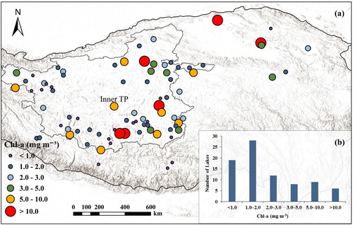
The annual mean Chl-a values of the studied lakes in the period of 2003–2017 are presented in Figure 2 and Table A1. The long-term mean Chl-a of the studied lakes ranged from 0.3 to 23.0 mg m⁻³, with a mean (±standard error) of 3.3  ±  4.3 mg m⁻³. Clearly, the majority (55/82) of selected lakes fitted the criteria of oligotrophic trophic class in terms of the Chl-a values (<2.6 mg m⁻³), according to the Carlson's trophic states classification scheme (i.e. oligotrophic: Chl-a <2.6 mg m⁻³; mesotrophic: 2.6 mg m⁻³ <Chl-a <20 mg m⁻³; and eutrophic 20 mg m⁻³ < Chl-a <55 mg m⁻³) (Carlson 2007). Others were all belonged to the mesotrophic level except for Ngangze Co, Keluke Lake and Ma’erxia Co, which were identified to have long-term mean Chl-a values close to or larger than 20.0 mg m⁻³. A clear spatial pattern is revealed is Figure 2. It can be seen that the majority of lakes with higher Chl-a values were located in the eastern and southern parts of the inner TP basin, as well as the northeastern TP region. In contrast, only a few lakes with Chl-a values above the mean level (i.e. 3.3 mg m⁻³) could be found in the western TP region.

Figure 2. (a) Distributions of long-term annual mean Chl-a of the examined lakes covering the TP over the period of 2003–2017. (b) The number of lakes characterized by different annual mean Chl-a levels.

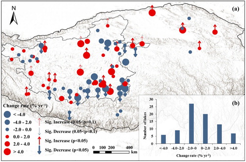
The distribution of the Chl-a change rate for the examined lakes is presented in Figure 3 and the exact value for each studied lake can be found in Table A1. It can be clearly seen that the majority (69/82) of lakes exhibited an absolute change trend of <4.0% yr⁻¹. Trend analysis indicated that 45.2% (19/42) of those lakes demonstrated a significant trend with p-values of <0.1, and 35.7% (15/42) of them had p-values of <0.05. Similarly, for lakes showing increasing trends, the percentages that experienced significant variation levels of 0.1 and 0.05 were 50.0% (20/40) and 37.5% (15/40), respectively. In general, the lakes demonstrating decreasing trends and the increasing trends were comparable in number but diverse in distribution pattern. While lakes with (significant) decreasing trends were concentrated in the southeastern part of the inner TP basin, lakes with (significant) increasing trends were distributed more evenly across the whole region, with a moderate aggregation in the northwestern inner TP basin as well as the eastern part of the entire TP region.

Figure 3. (a) Distributions of the annual Chl-a change rate for the examined lakes covering the TP for the period of 2003–2017. Lakes with a statistically significant change rate at a significance level of 0.05 were annotated with bold versions of ‘↑’ and ‘↓’, while those at a significance level of 0.1 but not at a significance level of 0.05 were annotated with light versions of ‘↑’ and ‘↓’. (b) The number of lakes characterized by different Chl-a change rate levels.

3.2. Long-term monthly means and variations in Chl-a

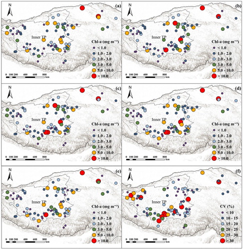
Figure 4 demonstrated the monthly mean Chl-a of the entire region from June to October, as well as the monthly coefficient of variance (CV, a result of the division of the mean by standard deviation) for the period of 2003–2017. The monthly median Chl-a for the studied lakes was generally close to one another (1.8–2.0 mg m⁻³). However, the seasonal discrepancy did exist in which August had the lowest number of lakes with Chl-a values of <1.0 mg m⁻³ and the highest number of lakes with Chl-a values of >10.0 mg m⁻³, while the situation in June and October was exactly the opposite. Despite of the seasonal discrepancy, the spatial pattern of monthly Chl-a in the overall region was consistent with the annual results stated above. In addition, the CV map (Figure 4) showed that lakes located in the western inner TP basin had higher monthly variations than the eastern TP inner basin, where more than half of the lakes in the western inner TP basin had CV values >20%, while CV values of the majority of lakes in the eastern inner TP basin were <20%.

Figure 4. (a-e) Distributions of long-term monthly mean Chl-a (a-e represent June-October, respectively) in the examined lakes covering the TP for the period of 2003–2017. (f) The CV between the long-term monthly mean Chl-a in panels a-e.

Figure 5 further reveals the monthly shift for each studied lake across the entire TP region. It is clearly presented that the lakes that had the lowest Chl-a in September and October were aggregated in the northwestern and northeastern parts of the TP region, respectively. In contrast, the south TP region was occupied by lakes with the lowest Chl-a observed from June to August. Statistically, approximately two-thirds of lakes reached minimum Chl-a levels in June and October. A different picture can be revealed when considering the spatial distribution of the months in which lakes presented the highest monthly Chl-a levels. In general, the number of lakes that had the highest Chl-a in August was the largest, accounting for 30.5% (25/82) of the total lakes. In terms of the spatial pattern, while the majority of lakes with the highest Chl-a in June and July were concentrated in the eastern (especially northeastern) inner TP basin, the lakes demonstrating the highest Chl-a in September and October were primarily located in the southern and northwestern inner TP basin. For lakes showing the highest Chl-a in August, their distributions were relatively scattered across the whole region, although a higher proportion can be observed in the south.

Figure 5. The months in which lakes exhibit the (a) lowest mean Ch-a and (b) highest mean Chl-a for the period of 2003–2017, as well as the corresponding histograms of the number of lakes in different months.

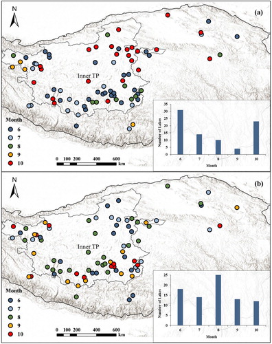
In summary, the monthly climatologies (i.e. long term monthly mean) of lakes in the TP region are revealed as follows: In June and July, when the Chl-a values in more than 60% of the studied lakes located in the southern TP began to increase from the bottom, the lakes in the northwestern inner TP basin had already reached their maximum levels throughout the examined months. In August, more than 30% of lakes spreading across the whole region reached the maximum. In contrast, only a few lakes located in the southeastern TP inner basin exhibited the Chl-a minima during this month. In September and October, a large proportion of lakes in the southern and northwestern inner TP basin show large Chl-a values, while many lakes in the northeastern and northwestern inner TP basin demonstrated minimum Chl-a concentrations accordingly.

3.3. Correlations with lake sizes and four environmental factors

Analysis showed that the Chl-a of 35.4% (29/82) of studied lakes were strongly correlated with lake area, indicating that profound alternations in aquatic environments would occur during the process of expansion or shrinkage of lakes. Indeed, the dynamics of lakes in area/volume is a combined effect of various environmental factors, which would simultaneously influence the aquatic environment. However, the variations in Chl-a may not be fully explained by the expansion/shrinkage of lakes alone. Other environmental factors may also play essential roles. Figure 6 demonstrates the percentages of lakes that exhibited significant correlations between Chl-a and the other four environmental factors. The corresponding correlation coefficients for each lake are displayed in Table A1. Except for lake size, the Chl-a value of 20.7% (17/82) of lakes was significantly correlated with wind speed, while the values for LSWT, ICD and surface runoff were 18.3% (15/82), 23.1% (9/39) and 23.2% (19/82), respectively, with both positive and negative correlations being identified. Indeed, the impacts of those environmental factors on lake Chl-a are complex and may vary across different lakes. For example, wind strongly impacts the mixing of nutrients and water column turbulence. A previous study showed that a high wind speed facilitates a high Chl-a concentration, in a way that high wind deepened the mixed layer, leading to a greater entrainment of deep nutrients and Chl-a being brought to the surface (Kahru et al. 2010). However, high wind speeds were also found to not favor water stability and thus disrupted the accumulation of phytoplankton, indicating a negative impact on Chl-a (Cao et al. 2006; Zhang et al. 2012). Such a diversity of impacts may also exist in other environmental factors. It is acknowledged that mechanism-based modeling on lacustrine Chl-a dynamics of this region would better facilitate our understanding of the specific roles these environmental factors play in regulating lake Chl-a.

Figure 6. The percentages of lakes with significant correlations (blue for p < 0.05 and red for p < 0.1) between different environmental factors and annual mean Chl-a.

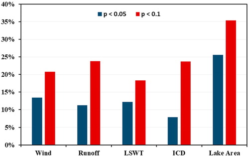
In summary, lake size and other environmental factors were found to be important factors affecting Chl-a. Statistically, 70% of the variations in lake Chl-a were significantly associated with at least one of the five environmental drivers studied above. Although the analysis conducted above could only explain part of the Chl-a variations, the analysis indicates relative importance of the influencing factors. Particularly, the expansion or shrinkage of lakes in this region has played an important role in the variations of Chl-a.

4. Discussion

4.1. Potential impacts from other forces

Except for the environmental factors discussed above, there are some environmental factors that are hard to quantify (owing to a lack of data) but may also exert significant influences on the dynamics of lake Chl-a, including salinity, glacial melt, nutrients and other possible driving factors.

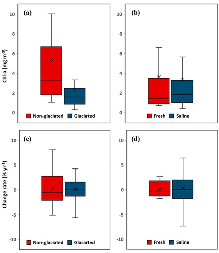
Glacial melt introduces cold water along with nutrients, providing the minerals required for algae growth while cooling the lake surface temperature and reducing light availability for phytoplankton simultaneously. To investigate the impact of glacial melting, the studied lakes were portioned into two groups (status of glaciation for each lake is presented in Table A1), with one containing glaciated lakes and the other consisting of non-glaciated lakes (Figure 7a, c). Considering the long-term annual Chl-a mean, a significant difference (p = 0.033) could be identified among the two groups based on t-test. Compared with groups that were made up of non-glaciated lakes, lakes fed by glaciers had lower mean (5.4 mg m⁻³ for non-glaciated lakes and 2.8 mg m⁻³ for glaciated lakes) and median (3.3 mg m⁻³ for non-glaciated lakes and 1.7 mg m⁻³ for glaciated lakes) Chl-a values. In terms of the change trend, the non-glaciated lakes exhibited a larger variations in both increasing rate and decreasing rate than the glaciated lakes while no significant difference between the two groups was identified. Overall, the results suggested a potential negative impact of glacier meltwater on Chl-a concentrations for lakes in the TP region, from the perspectives of long-term annual mean values. This result may be achieved mainly through the cooling effects of glacier meltwater on phytoplankton living in lakes.

Figure 7. Boxplot of the impact of (a) glacial melt and (b) salinity on Chl-a in the studied lakes.

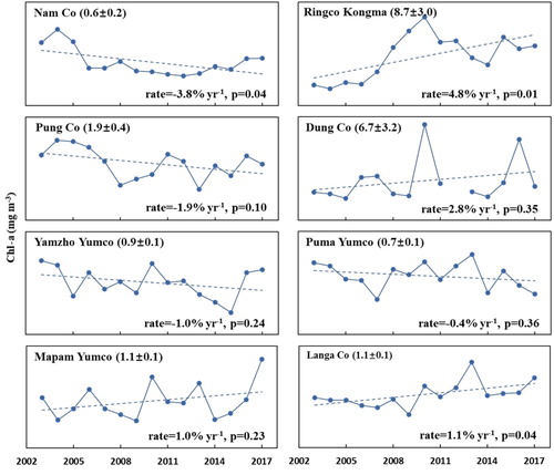
To further investigate the contribution of glacier meltwater to the fluctuation of lake Chl-a, several pairs of lakes in close proximity to each other are displayed for comparison (see Figure 8). The annual changes in Chl-a for Nam Co and Ringco Kongma were first compared, with the former receiving glacier meltwater and the latter not receiving meltwater. Overall, Nam Co (glacier-fed) experienced a significantly decreasing trend during the study period at a rate of −3.8% yr⁻¹. In contrast, Ringco Kongma (non-glacier-fed) experienced a significantly increasing trend during the same period at a rate of 4.8% yr⁻¹. Since the two lakes are geographically close to each other (with a distance of ∼60 km), the climatic influence on these lakes can be minimized. In this case, the difference in Chl-a values between the lakes may primarily be induced by glacier meltwater (Song et al. 2014b). A similar situation could be observed for Lake Pung Co (glacier-fed) and Dung Co (non-glacier-fed). While the Chl-a values of the former lake decreased, an increasing trend could be observed for the latter, suggesting a potential negative impact of glaciers on lake Chl-a. For comparison, Yamzho Yumco and Puma Yumco are a pair of lakes that are not only located in spatially adjacent areas but also receive meltwater from glaciers. These two lakes exhibited comparable mean Chl-a values as well as similar decreasing trends, which was also true for Lake Mapam Yumco and Langa Co. The analysis above further confirmed the important role of glacier meltwater in modulating lake Chl-a. For the lakes in the TP region, the glacier meltwater primarily lowers the lake Chl-a levels.

Figure 8. Interannual variation of Chl-a and trend (% yr⁻¹) for the period of 2003–2017 for several pairs of lakes that are in close proximity. Lake names and long term annual mean Chl-a values (mg m⁻³) are presented in the upper left corner, while change rates and corresponding p-values are displayed in the bottom right corner.

Another potentially influential environmental factor is salinity. Salinity is used to describe the content of dissolved inorganic salt in water bodies. Saline water may also exert an influence on Chl-a concentrations through possible regulation of cell division and algae development (Ding et al. 2013; Desmit, Ruddick, and Lacroix 2015; Lin et al. 2017). To investigate the actual impact of salinity on the lakes in the TP, group difference analyses were conducted (Figure 7b, 7d). Note that the status of salinity for each lake is presented in Table A1. The annual mean Chl-a was 4.0 ± 4.9 mg m⁻³ for fresh lakes and 3.8 ± 4.3 mg m⁻³ for saline lakes, which was a minor difference. Statistically nonsignificant group difference results based on a t-test in view of either long-term annual mean values (p = 0.848) or long-term trends (p = 0.349 for an increasing trend and p = 0.103 for a decreasing trend) further confirmed the limited impact of salinity on lake Chl-a in the TP.

In terms of nutrient, previous studies have revealed nutrient (especially for nitrogen and phosphorous) as one of the most important factors because of their evident impact on facilitating phytoplankton growth (Warner and Lesht 2015; Zhang et al. 2016; Rowe et al. 2017; Huang et al. 2019). However, due to the data limitation on nutrient loads discharged in lakes, the direct impact of nutrients cannot be assessed in this study. In this case, surface runoff and glacier were chosen to partially reflect the potential impact of nutrients, as surface runoff and glacier meltwater are the most important nutrient inputs for many lakes in the TP region.

In addition, solar radiation, water turbidity and hydrological conditions including water level and water residence time are also believed to be potential factors regulating lake Chl-a (Wu et al. 2013; Feng et al. 2014; Wang et al. 2015; Yang et al. 2016; Cha et al. 2017; Blauw et al. 2018; Liu, Feng, and Wang 2019). In general, these factors take effect through either direct or indirect regulations on the availability of light or nutrients that are indispensable for phytoplankton growth. In addition, there may be other unknown factors that play significant roles; however, the underlying mechanism remains to be explored.

4.2. Validity and uncertainty of remotely sensed Chl-a

Due to the harsh environment, as well as the limited accessibility for cruise surveys, in situ measurements of Chl-a throughout lakes in the TP are rare. To our knowledge, an intensive field observation was conducted in 2017, and the relevant dataset was available in the National Tibetan Plateau Data Center (http://data.tpdc.ac.cn). The water quality dataset contained vertical profiles of ∼30 observation points in lakes across the TP. However, due to the presence of clouds and other nonoptimal observational conditions, daily valid observational coverage is unsatisfactory, leading to limited match-ups between in situ data and satellite-derived Chl-a. In practice, only 10 valid match-ups with day gaps ≤3 days were extracted successfully from the 30 in situ data samples, which was inadequate for model development and validation. In fact, the function of the in situ data in most cases was an adjustment of the empirical coefficients of the Chl-a algorithm, which had little impact on the calculated long-term Chl-a trend. Such conclusion has been confirmed by Lewis (Lewis, van Dijken, and Arrigo 2020) in the study of Chl-a variations in Arctic Ocean where the standard empirical algorithms adopted by NASA showed consistent trend with their tuned algorithm. In addition, our validation results showed that the R² was 0.79 and a significant correlation (p < 0.001 through the Spearman's rank correlation, which are widely used to describe nonlinear correlation relationship) can be identified between in-situ Chl-a and satellite-derived Chl-a. Since the number of match-up was not adequate and the temporal differences between satellite and in situ observations are up to 3 days, we did not tune the empirical coefficients of the standard NASA algorithm. Nevertheless, the results supported our opinion that the trend captured by the Chl-a product were consistent with the ‘true value’. Therefore, since the major objective of this study is to examine the variations of lake Chl-a rather than the exact Chl-a values, the results demonstrated here would not be strongly influenced by the lack of sufficient in situ data to conduct re-calibration and validation of the satellite Chl-a retrieving algorithm.

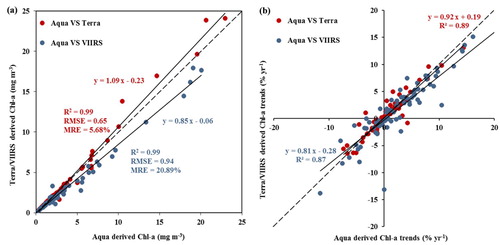
On the other hand, the capability of Aqua-derived Chl-a observations in capturing Chl-a change trend can also be partially assessed through a comparison with similar satellite products, including MODIS Terra and VIIRS. Because data from VIIRS are not available until 2012, long-term annual mean Chl-a in the period of 2003–2017 were applied for comparison of MODIS Aqua and Terra, while the 2012–2017 long-term annual mean data were used for comparison of MODIS Aqua and VIIRS. The processing procedures were the same for all satellites, and the results are shown in Figure 9. The R² was 0.99 for both correlations in terms of long-term annual mean (Figure 9a), indicating high consistency between the Chl-a derived from the three satellites. The comparison results in the Chl-a trend (Figure 9b) further confirmed the high level of agreement among the three instruments, with R² = 0.89 and 0.87, respectively. In addition, a detailed examination for each lake showed that the annual mean Chl-a of 96.3% in the studied lakes exhibited a significant correlation between MODIS Aqua and Terra, while the percentage is 81.7% in terms of MODIS Aqua and VIIRS. In fact, the percentage for the latter may be higher in the future once longer time series of data for VIIRS are available for correlation analysis. Although Chl-a values derived from MODIS Terra were consistently larger than those from MODIS Aqua and Chl-a derived from VIIRS exhibited systematically lower values, the uncertainties among the three satellites, represented either as RMSE or MRE, were moderate. In general, Chl-a observed from MODIS Aqua exhibited higher proximity with those obtained from Terra (RMSE = 0.65 mg m⁻³, MRE = 5.68%) than those from VIIRS (RMSE = 0.94 mg m⁻³, MRE = 20.89%). This finding is most likely because the instrument and algorithmic designs of Aqua and Terra are similar except for the 3 h temporal differences; however, all three types of differences exist among MODIS Aqua and VIIRS.

Figure 9. Comparison of (a) long-term annual mean Chl-a and (b) long-term Chl-a trend of 82 examined lakes derived from MODIS Aqua with MODIS Terra and VIIRS.

In summary, the Chl-a derived from the three satellites exhibited high consistency for most studied lakes (with an average R² = 0.84) in the TP, which confirmed the long-term trend of Chl-a variations in this region. Since the trend of the dynamics and the broad picture rather than the absolute values of lake Chl-a are of more importance in improving our understanding of Chl-a distribution and lake ecology in the TP region, it is reasonable to conclude that the remotely sensed results in this study were fairly reliable and valuable.

Several uncertainty sources that may exert impacts on Chl-a estimations can be identified in this study. The first type of uncertainty is closely related to data gaps under unfavorable measurement conditions. Under conditions of cloud cover, straylight, sun glint and imperfect solar/viewing angles, the validity of Chl-a retrievals are profoundly diminished and typically discarded according to corresponding data quality flags. In practice, a 7 × 5 pixel straylight mask is implemented for data exclusion in SeaDAS. However, a large quantity of valid data would also be screened out during this process, resulting in a reduction in valid coverage as well as an increase in uncertainty because less valid data can be used for zonal statistics (Feng and Hu 2015). Such a problem can be partially addressed by applying Feng and Hu's data recovery method, where a 3 × 3, rather than a standard 7 × 5, pixel window was implemented for low-quality data screening, leading to an average of approximately 40% increases in valid observations globally (Hu et al. 2019). This method has been proven to be efficient in recovering valid data close to nonoptimal observational conditions and hence reducing product uncertainty without compromising data quality (Feng and Hu 2016; Hu et al. 2019).

Another type of uncertainty may be induced by residual errors from atmospheric correction (AC) algorithms. Indeed, it is ultimately difficult to remove the effects of aerosols in AC procedures due to the distinct variations in aerosol properties; hence, the residual errors introduced by aerosols are embedded in current AC methods (Liu et al. 2015; Pahlevan et al. 2017; Liu et al. 2019). However, as the TP is characterized by nominal human activities, such an impact may be limited (Feng et al. 2019). On the other hand, the standard AC approach (Gordon and Wang 1994) is established with the assumption that the water-leaving radiance (Lw) in the two near-infrared (NIR) bands is close to zero, which works well for most open oceans (McClain 2009). As the turbidity increases, it is argued that the water signal in the NIR bands may no longer be zero, and the shortwave infrared (SWIR) bands are recommended (Wang and Shi 2007) for AC instead because the Lw (SWIR) in this case can be zero (due to high absorption in SWIR bands). However, using Chesapeake Bay as an example, Werdell et al. discovered that extra errors in the derivation of Lw(λ) would be introduced into the SWIR-based AC owing to poor signal-to-noise (SNR) ratios inherent in the SWIR bands of MODIS Aqua (Werdell, Franz, and Bailey 2010). Such deficiency in the design of MODIS Aqua instruments restricted the applicability of SWIR-based AC. In addition, many lakes in the TP are relatively clearer than Chesapeake Bay, leading to more satisfactory results in the NIR-based AC. Therefore, although potential uncertainties may exist, the NIR-based standard AC was used in this study. Moreover, the look-up tables for AC embedded in SeaDAS were based on sea level, while the current study area has an altitude of >4000 m that may also increase the uncertainties in AC processes. However, the accuracy of this currently used dataset has been confirmed through comparison of MODIS Rrs corrected in the AC process and in situ samplings in Qinghai Lake conducted by Feng et al (Feng et al. 2019). Both the magnitude and spectral shape of MODIS Rrs are observed to be highly consistent with the in situ measurements (see Figure 8 in [Feng et al. 2019]).

Other sources that may contribute to estimation uncertainties include the bottom reflectance as well as the optical properties impacted by water constituents like colored dissolved organic matter (CDOM). Bottom reflectance is often regarded as an essential contributor to the water-leaving radiance for optically shallow inland waters, exerting negative impacts on the accuracies of bio-optical algorithms (Lee et al. 2001; Li et al. 2017). However, for optically deep inland waters, the light reflected by bottom sediments is significantly attenuated by the water column as well as its constituents and is expected to exert a negligible impact on the total water-leaving signals at a certain depth (Dogliotti et al. 2015). Since many examined lakes in the TP have an average depths of tens of meters, the uncertainty caused by bottom reflectance, if present, would be limited under these circumstances (Wang and Dou 1998). For the optical disturbance of nonliving water constituents, it is acknowledged that those substances may induce variant bias among different lakes in terms of the estimation of absolute Chl-a values. However, similar to the uncertainty introduced by AC, it is believed that such an influence would be less significant in the evaluation of long-term Chl-a fluctuations across oceans and comparably in inland waters less impacted by human activities across the TP region (Hu et al. 2019).

4.3. Future implications

The results of this study provide a baseline for studying the biogeochemical characteristics of lakes in the TP and have significant implications for understanding the responses of lake Chl-a to future climate changes. Given the current climate variations and future trends, majority of lakes in this region have experienced rapid expansions since the 2000s and will continue to expand for a certain period (Sun et al. 2018b). These changes would in turn result in considerable alterations in the aquatic environment. Functioning as the Asian Water Tower, water security in the TP is critical and thus drawing increasing attention and scientific investment from society and governments. In the future, it is expected that denser in situ observation networks will be developed in this region, along with the initiation of new satellites with higher spatial/temporal/spectral resolutions and mature cross-sensor calibrations among different instruments for multiple data infusion. Under such conditions, a more detailed understanding of the biogeochemical properties of lakes will be achieved, which is of great significance in addressing the potential risks induced by variations in inland water quality and maintaining water security in this region.

5. Conclusion

In this study, the interannual and monthly changes of Chl-a in various lakes across the entire TP region was quantified using multiple ocean color products. A total of 82 lakes were investigated in the period of 2003–2017. The derived Chl-a from MODIS Aqua exhibited high consistency with the values retrieved from MODIS Terra and VIIRS, indicating the validity of the results in revealing spatiotemporal variations and change trend in lake Chl-a across the TP. A clear spatial pattern in the long-term annual mean Chl-a can be observed, where lakes with high Chl-a values were primarily distributed in the eastern and southern inner TP basin together with the northeastern part of the whole TP region. In term of long-term trends, nearly half of the lakes were observed to experience a significant change trend during the study period. Overall, lakes with (significantly) decreasing trends were primarily located in the southeastern part of the inner TP basin, while the northwestern inner TP basin and the eastern part of the entire TP region were mainly occupied by lakes manifesting (significantly) increasing trends. Analysis of monthly mean values indicated a higher monthly variation for lakes located in the western inner TP basin. Statistically, a large proportion (approx. 65.9%) of the lakes represented the lowest Chl-a in June or October. In contrast, the percentage of lakes presenting the highest Chl-a in August is the largest, accounting for 30.5% of the total numbers with a scatter distribution across the whole region.

The Chl-a values in 35.4% of the lakes studied were strongly correlated with the dynamics of lake area. Another four environmental factor, wind speed, ICD, LSWT and surface runoff were also found contribute to the changes of Chl-a in lakes. In addition, the Chl-a levels could be lowered by glacier meltwater while there was no significant difference in Chl-a values between saline and fresh lakes. In summary, the influence of environmental factors on Chl-a is complicated and may behave differently for individual lakes. Further research focusing on the specific role of these factors as well as other unexplored factors requires mechanism-based modeling equipped with more comprehensive datasets. Nevertheless, this study demonstrates the applicability of satellite remote sensing in retrieving regional-scale Chl-a data, and the dataset is valuable for lake ecology monitoring and water security in this unique region.

Acknowledgements

This work was supported by the Strategic Priority Research Program of the Chinese Academy of Sciences (XDA20060402), the Second Tibetan Plateau Scientific Expedition and Research Program (2019QZKK0202), the National Natural Science Foundation of China (91747204and 41971304), the Shenzhen Science and Technology Innovation Committee (JCYJ20190809155205559), and the Colleges Pearl River Scholar FundedScheme 2018. The gridded wind speed dataset used in this study originated from the China Meteorological Forcing Dataset (CMFD), which was developed by the Data Assimilation and Modeling Center for Tibetan Multi-spheres, Institute of Tibetan Plateau Research of Chinese Academy of Sciences (https://data.tpdc.ac.cn/en/data/8028b944-daaa-4511-8769-965612652c49/). The ocean color data was obtained from NASA Ocean Biology Processing Group (OBPG) (https://oceancolor.gsfc.nasa.gov/cms/) and the Landsat imagery was provided by USGS EROS Data Center and NASA (https://glovis.usgs.gov/). We also thanked Dr. Changqing Ke for providing the lake ice cover duration data.

Disclosure statement

No potential conflict of interest was reported by the author(s).

Additional information

Funding

This work was supported by the Strategic Priority Research Program of the Chinese Academy of Sciences (XDA20060402), the Second Tibetan Plateau Scientific Expedition and Research Program (2019QZKK0202), the National Natural Science Foundation of China (91747204 and 4197130), the Shenzhen Science and Technology Innovation Committee (JCYJ20190809155205559), and the Colleges Pearl River Scholar FundedScheme 2018.

References

- Behrenfeld, Michael J., and Emmanual Boss. 2006. “Beam Attenuation and Chlorophyll Concentration as Alternative Optical Indices of Phytoplankton Biomass.” Journal of Marine Research 64 (3): 431–451.
- Blauw, Anouk N., Elisa Benincà, Remi W.P.M. Laane, Naomi Greenwood, and Jef Huisman. 2018. “Predictability and Environmental Drivers of Chlorophyll Fluctuations Vary across Different Time Scales and Regions of the North Sea.” Progress in Oceanography 161 (February): 1–18. doi:10.1016/j.pocean.2018.01.005.
- Cai, Yu, Chang-Qing Ke, Xingong Li, Guoqing Zhang, Zheng Duan, and Hoonyol Lee. 2019. “Variations of Lake Ice Phenology on the Tibetan Plateau From 2001 to 2017 Based on MODIS Data.” Journal of Geophysical Research: Atmospheres 124 (2): 825–843. doi:10.1029/2018JD028993.
- Cao, Huan-Sheng, Fan-Xiang Kong, Lian-Cong Luo, Xiao-Li Shi, Zhou Yang, Xiao-Feng Zhang, and Yi Tao. 2006. “Effects of Wind and Wind-Induced Waves on Vertical Phytoplankton Distribution and Surface Blooms of Microcystis Aeruginosa in Lake Taihu.” Journal of Freshwater Ecology 21 (2): 231–238.
- Carey, Cayelan C., Bas W. Ibelings, Emily P. Hoffmann, David P. Hamilton, and Justin D. Brookes. 2012. “Eco-Physiological Adaptations That Favour Freshwater Cyanobacteria in a Changing Climate.” Water Research 46 (5): 1394–1407.
- Carlson, R. E. 2007. “Estimating Trophic State.” LakeLine 27 (1): 25–28.
- Carranza, Magdalena M., and Sarah T. Gille. 2015. “Southern Ocean Wind-driven Entrainment Enhances Satellite Chlorophyll-a through the Summer.” Journal of Geophysical Research: Oceans 120 (1): 304–323.
- Cha, YoonKyung, Kyung Hwa Cho, Hyuk Lee, Taegu Kang, and Joon Ha Kim. 2017. “The Relative Importance of Water Temperature and Residence Time in Predicting Cyanobacteria Abundance in Regulated Rivers.” Water Research 124: 11–19.
- Desmit, Xavier, Kevin Ruddick, and Geneviève Lacroix. 2015. “Salinity Predicts the Distribution of Chlorophyll a Spring Peak in the Southern North Sea Continental Waters.” Journal of Sea Research 103 (September): 59–74. doi:10.1016/j.seares.2015.02.007.
- Ding, Lanping, Yuanyuan Ma, Bingxin Huang, and Shanwen Chen. 2013. “Effects of Seawater Salinity and Temperature on Growth and Pigment Contents in Hypnea Cervicornis J. Agardh (Gigartinales, Rhodophyta).” BioMed Research International 2013: 1–10. doi:10.1155/2013/594308.
- Dogliotti, Ana Inés, K. G. Ruddick, B. Nechad, D. Doxaran, and E. Knaeps. 2015. “A Single Algorithm to Retrieve Turbidity from Remotely-Sensed Data in All Coastal and Estuarine Waters.” Remote Sensing of Environment 156: 157–168.
- Eadie, Brian J, David J Schwab, Thomas H Johengen, Peter J Lavrentyev, Gerald S Miller, Ruth E Holland, George A Leshkevich, Margaret B Lansing, Nancy R Morehead, and John A Robbins. 2002. “Particle Transport, Nutrient Cycling, and Algal Community Structure Associated with a Major Winter-Spring Sediment Resuspension Event in Southern Lake Michigan.” Journal of Great Lakes Research 28 (3): 324–337.
- Feng, Lian, and Chuanmin Hu. 2015. “Comparison of Valid Ocean Observations between MODIS Terra and Aqua over the Global Oceans.” IEEE Transactions on Geoscience and Remote Sensing 54 (3): 1575–1585.
- Feng, Lian, and Chuanmin Hu. 2016. “Cloud Adjacency Effects on Top-of-Atmosphere Radiance and Ocean Color Data Products: A Statistical Assessment.” Remote Sensing of Environment 174: 301–313. doi:10.1016/j.rse.2015.12.020.
- Feng, Lian, Chuanmin Hu, Xingxing Han, Xiaoling Chen, and Lin Qi. 2014. “Long-Term Distribution Patterns of Chlorophyll-a Concentration in China’s Largest Freshwater Lake: MERIS Full-Resolution Observations with a Practical Approach.” Remote Sensing 7 (1): 275–299. doi:10.3390/rs70100275.
- Feng, Lian, Junguo Liu, Tarig A. Ali, Junsheng Li, Juan Li, and Xingxing Kuang. 2019. “Impacts of the Decreased Freeze-up Period on Primary Production in Qinghai Lake.” International Journal of Applied Earth Observation and Geoinformation 83 (January): 101915. doi:10.1016/j.jag.2019.101915.
- Gons, Herman J., Martin T. Auer, and Steven W. Effler. 2008. “MERIS Satellite Chlorophyll Mapping of Oligotrophic and Eutrophic Waters in the Laurentian Great Lakes.” Remote Sensing of Environment 112 (11): 4098–4106.
- Gordon, Howard R, and Menghua Wang. 1994. “Retrieval of Water-Leaving Radiance and Aerosol Optical Thickness over the Oceans with SeaWiFS: A Preliminary Algorithm.” Applied Optics 33 (3): 443–452.
- Guildford, Stephanie J, and Robert E Hecky. 2000. “Total Nitrogen, Total Phosphorus, and Nutrient Limitation in Lakes and Oceans: Is There a Common Relationship?” Limnology and Oceanography 45 (6): 1213–1223.
- Guo, Linan, Yanhong Wu, Hongxing Zheng, Bing Zhang, Junsheng Li, Fangfang Zhang, and Qian Shen. 2018. “Uncertainty and Variation of Remotely Sensed Lake Ice Phenology across the Tibetan Plateau.” Remote Sensing 10 (10): 1534. doi:10.3390/rs10101534.
- He, Jie, Kun Yang, Wenjun Tang, Hui Lu, Jun Qin, Yingying Chen, and Xin Li. 2020. “The First High-Resolution Meteorological Forcing Dataset for Land Process Studies over China.” Scientific Data 7 (1): 25. doi:10.1038/s41597-020-0369-y.
- Hodges, Ben R, Jörg Imberger, Angelo Saggio, and Kraig B Winters. 2000. “Modeling Basin-Scale Internal Waves in a Stratified Lake.” Limnology and Oceanography 45 (7): 1603–1620.
- Horvat, Christopher, David Rees Jones, Sarah Iams, David Schroeder, Daniela Flocco, and Daniel Feltham. 2017. “The Frequency and Extent of Sub-Ice Phytoplankton Blooms in the Arctic Ocean.” Science Advances 3 (3): e1601191.
- Hu, Chuanmin, Lian Feng, Zhongping Lee, Bryan A. Franz, Sean W. Bailey, P. Jeremy Werdell, and Christopher W. Proctor. 2019. “Improving Satellite Global Chlorophyll a Data Products Through Algorithm Refinement and Data Recovery.” Journal of Geophysical Research: Oceans 124 (3): 1524–1543. doi:10.1029/2019JC014941.
- Hu, Chuanmin, Zhongping Lee, and Bryan Franz. 2012. “Chlorophyll Aalgorithms for Oligotrophic Oceans: A Novel Approach Based on Three-Band Reflectance Difference.” Journal of Geophysical Research: Oceans 117 (C1): C01011.1–C01011.25.
- Huang, Changchun, Yunlin Zhang, Tao Huang, Hao Yang, Yunmei Li, Zhigang Zhang, Mengying He, Zhujun Hu, Ting Song, and A-xing Zhu. 2019. “Long-Term Variation of Phytoplankton Biomass and Physiology in Taihu Lake as Observed via MODIS Satellite.” Water Research 153: 187–199.
- Huffman, George J., David T. Bolvin, Eric J. Nelkin, David B. Wolff, Robert F. Adler, Guojun Gu, Yang Hong, Kenneth P. Bowman, and Erich F. Stocker. 2007. “The TRMM Multisatellite Precipitation Analysis (TMPA): Quasi-Global, Multiyear, Combined-Sensor Precipitation Estimates at Fine Scales.” Journal of Hydrometeorology 8 (1): 38–55.
- Jiang, Liguang, Karina Nielsen, Ole B. Andersen, and Peter Bauer-Gottwein. 2017. “Monitoring Recent Lake Level Variations on the Tibetan Plateau Using CryoSat-2 SARIn Mode Data.” Journal of Hydrology 544: 109–124. doi:10.1016/j.jhydrol.2016.11.024.
- Kahru, M., S. T. Gille, R. Murtugudde, P. G. Strutton, M. Manzano-Sarabia, H. Wang, and B. G. Mitchell. 2010. “Global Correlations between Winds and Ocean Chlorophyll.” Journal of Geophysical Research: Oceans 115 (C12): C12040.
- Kalff, J. 2002. Limnology: Inland Water Ecosystems. Prentice Hall. https://books.google.com.hk/books?id=DzgUAQAAIAAJ.
- Kong, Lingyang, Xiangdong Yang, Giri Kattel, N. J. Anderson, and Zhujun Hu. 2017. “The Response of Cladocerans to Recent Environmental Forcing in an Alpine Lake on the SE Tibetan Plateau.” Hydrobiologia 784 (1): 171–185. doi:10.1007/s10750-016-2868-6.
- Krause, P., S. Biskop, J. Helmschrot, W.-A. Flügel, S. Kang, and T. Gao. 2010. “Hydrological System Analysis and Modelling of the Nam Co Basin in Tibet.” Advances in Geosciences 27 (August): 29–36. doi:10.5194/adgeo-27-29-2010.
- Kropáček, J., F. Maussion, F. Chen, S. Hoerz, and V. Hochschild. 2013. “Analysis of Ice Phenology of Lakes on the Tibetan Plateau from MODIS Data.” The Cryosphere 7 (1): 287–301. doi:10.5194/tc-7-287-2013.
- Kuang, Xingxing, and Jiu Jimmy Jiao. 2016a. “Review on Climate Change on the Tibetan Plateau during the Last Half Century.” Journal of Geophysical Research 121 (8): 3979–4007. doi:10.1002/2015JD024728.
- Kuang, Xingxing, and Jiu Jimmy Jiao. 2016b. “Review on Climate Change on the Tibetan Plateau during the Last Half Century.” Journal of Geophysical Research: Atmospheres 121 (8): 3979–4007. doi:10.1002/2015JD024728.
- Lee, Zhongping, Kendall L Carder, Robert F Chen, and Thomas G Peacock. 2001. “Properties of the Water Column and Bottom Derived from Airborne Visible Infrared Imaging Spectrometer (AVIRIS) Data.” Journal of Geophysical Research: Oceans 106 (C6): 11639–11651.
- Lei, Yanbin, and Kun Yang. 2017. “The Cause of Rapid Lake Expansion in the Tibetan Plateau: Climate Wetting or Warming?” Wiley Interdisciplinary Reviews: Water 4 (6): e1236. doi:10.1002/wat2.1236.
- Lei, Yanbin, Kun Yang, Bin Wang, Yongwei Sheng, Broxton W. Bird, Guoqing Zhang, and Lide Tian. 2014. “Response of Inland Lake Dynamics over the Tibetan Plateau to Climate Change.” Climatic Change 125 (2): 281–290. doi:10.1007/s10584-014-1175-3.
- Lewis, K. L., G. L. van Dijken, and Kevin R. Arrigo. 2020. “Changes in Phytoplankton Concentration, Not Sea Ice, Now Drive Increased Arctic Ocean Primary Production.” Science 202 (July): 198–202.
- Li, Jiwei, Qian Yu, Yong Q Tian, and Brian L Becker. 2017. “Remote Sensing Estimation of Colored Dissolved Organic Matter (CDOM) in Optically Shallow Waters.” ISPRS Journal of Photogrammetry and Remote Sensing 128: 98–110.
- Lin, Li, Lei Dong, Zhen Wang, Chao Li, Min Liu, Qingyun Li, and John C Crittenden. 2020. “Hydrochemical Composition, Distribution, and Sources of Typical Organic Pollutants and Metals in Lake Bangong Co, Tibet.” Environmental Science and Pollution Research.
- Lin, Qiuqi, Lei Xu, Juzhi Hou, Zhengwen Liu, Erik Jeppesen, and Bo-Ping Han. 2017. “Responses of Trophic Structure and Zooplankton Community to Salinity and Temperature in Tibetan Lakes: Implication for the Effect of Climate Warming.” Water Research 124 (November): 618–629. doi:10.1016/j.watres.2017.07.078.
- Liu, Xia, Jianfeng Feng, and Yuqiu Wang. 2019. “Chlorophyll a Predictability and Relative Importance of Factors Governing Lake Phytoplankton at Different Timescales.” Science of The Total Environment 648 (January): 472–480. doi:10.1016/j.scitotenv.2018.08.146.
- Liu, Ge, Yunmei Li, Heng Lyu, Shuai Wang, Chenggong Du, and Changchun Huang. 2015. “An Improved Land Target-Based Atmospheric Correction Method for Lake Taihu.” IEEE Journal of Selected Topics in Applied Earth Observations and Remote Sensing 9 (2): 793–803.
- Liu, Huizeng, Qiming Zhou, Qingquan Li, Shuibo Hu, Tiezhu Shi, and Guofeng Wu. 2019. “Determining Switching Threshold for NIR-SWIR Combined Atmospheric Correction Algorithm of Ocean Color Remote Sensing.” ISPRS Journal of Photogrammetry and Remote Sensing 153: 59–73.
- Lyche-Solheim, Anne, Christian K. Feld, Sebastian Birk, Geoff Phillips, Laurence Carvalho, Giuseppe Morabito, Ute Mischke, Nigel Willby, Martin Søndergaard, and Seppo Hellsten. 2013. “Ecological Status Assessment of European Lakes: A Comparison of Metrics for Phytoplankton, Macrophytes, Benthic Invertebrates and Fish.” Hydrobiologia 704 (1): 57–74.
- McClain, Charles R. 2009. “A Decade of Satellite Ocean Color Observations.” Annual Review of Marine Science 1: 19–42.
- McFEETERS, S. K. 1996. “The Use of the Normalized Difference Water Index (NDWI) in the Delineation of Open Water Features.” International Journal of Remote Sensing 17 (7): 1425–1432. doi:10.1080/01431169608948714.
- O’Reilly, John E., Stéphane Maritorena, B. Greg Mitchell, David A. Siegel, Kendall L. Carder, Sara A. Garver, Mati Kahru, and Charles McClain. 1998. “Ocean Color Chlorophyll Algorithms for SeaWiFS.” Journal of Geophysical Research: Oceans 103 (C11): 24937–24953. doi:10.1029/98JC02160.
- Pahlevan, Nima, S. Sarkar, B. A. Franz, S. V. Balasubramanian, and J. He. 2017. “Sentinel-2 MultiSpectral Instrument (MSI) Data Processing for Aquatic Science Applications: Demonstrations and Validations.” Remote Sensing of Environment 201: 47–56.
- Pant, Ramesh Raj, Fan Zhang, Faizan Ur Rehman, Guanxing Wang, Ming Ye, Chen Zeng, and Handuo Tang. 2018. “Spatiotemporal Variations of Hydrogeochemistry and Its Controlling Factors in the Gandaki River Basin, Central Himalaya Nepal.” Science of the Total Environment 622: 770–782.
- Pi, Xuehui, Lian Feng, Weifeng Li, Dan Zhao, Xingxing Kuang, and Junsheng Li. 2020. “Water Clarity Changes in 64 Large Alpine Lakes on the Tibetan Plateau and the Potential Responses to Lake Expansion.” ISPRS Journal of Photogrammetry and Remote Sensing 170 (October): 192–204. doi:10.1016/j.isprsjprs.2020.10.014.
- Qi, Wei, Junguo Liu, and Deliang Chen. 2018a. “Evaluations and Improvements of GLDAS2.0 and GLDAS2.1 Forcing Data’s Applicability for Basin Scale Hydrological Simulations in the Tibetan Plateau.” Journal of Geophysical Research: Atmospheres 123 (23): 13,128–13,148. doi:10.1029/2018JD029116.
- Qi, Wei, Junguo Liu, and Deliang Chen. 2018b. “Evaluations and Improvements of GLDAS2.0 and GLDAS2.1 Forcing Data’s Applicability for Basin Scale Hydrological Simulations in the Tibetan Plateau.” Journal of Geophysical Research: Atmospheres 123: 23. doi:10.1029/2018JD029116.
- Qi, Wei, Junguo Liu, Jun Xia, and Deliang Chen. 2020. “Divergent Sensitivity of Surface Water and Energy Variables to Precipitation Product Uncertainty in the Tibetan Plateau.” Journal of Hydrology 581 (February): 124338. doi:10.1016/j.jhydrol.2019.124338.
- Qiao, Baojin, and Liping Zhu. 2017. “Differences and Cause Analysis of Changes in Lakes of Different Supply Types in the North-Western Tibetan Plateau.” Hydrological Processes 31 (15): 2752–2763. doi:10.1002/hyp.11215.
- Qiao, Baojin, Liping Zhu, and Ruimin Yang. 2019a. “Temporal-Spatial Differences in Lake Water Storage Changes and Their Links to Climate Change throughout the Tibetan Plateau.” Remote Sensing of Environment 222 (January): 232–243. doi:10.1016/j.rse.2018.12.037.
- Qiao, Baojin, Liping Zhu, and Ruimin Yang. 2019b. “Temporal-Spatial Differences in Lake Water Storage Changes and Their Links to Climate Change throughout the Tibetan Plateau.” Remote Sensing of Environment 222 (March): 232–243. doi:10.1016/j.rse.2018.12.037.
- Qiu, Jane. 2008. “China: The Third Pole.” Nature 454 (7203): 393–396. doi:10.1038/454393a.
- Ren, Jiao, Xiaoping Wang, Chuanfei Wang, Ping Gong, Xiruo Wang, and Tandong Yao. 2017. “Biomagnification of Persistent Organic Pollutants along a High-Altitude Aquatic Food Chain in the Tibetan Plateau: Processes and Mechanisms.” Environmental Pollution 220 (January): 636–643. doi:10.1016/j.envpol.2016.10.019.
- Rodell, Matthew, P. R. Houser, U. E. A. Jambor, J. Gottschalck, K. Mitchell, C.-J. Meng, K. Arsenault, B. Cosgrove, J. Radakovich, and M. Bosilovich. 2004. “The Global Land Data Assimilation System.” Bulletin of the American Meteorological Society 85 (3): 381–394.
- Rose, Kevin C., David P. Hamilton, Craig E. Williamson, Chris G. McBride, Janet M. Fischer, Mark H. Olson, Jasmine E. Saros, Mathew G. Allan, and Nathalie Cabrol. 2014. “Light Attenuation Characteristics of Glacially-Fed Lakes.” Journal of Geophysical Research-Biogeosciences 119 (7): 1446–1457. doi:10.1002/2014JG002674.
- Rowe, Mark D, Eric J Anderson, Henry A Vanderploeg, Steven A Pothoven, Ashley K Elgin, Jia Wang, and Foad Yousef. 2017. “Influence of Invasive Quagga Mussels, Phosphorus Loads, and Climate on Spatial and Temporal Patterns of Productivity in Lake Michigan: A Biophysical Modeling Study.” Limnology and Oceanography 62 (6): 2629–2649.
- Sayers, Michael J., Amanda G. Grimm, Robert A. Shuchman, Andrew M. Deines, David B. Bunnell, Zachary B. Raymer, Mark W. Rogers, Whitney Woelmer, David H. Bennion, and Colin N. Brooks. 2015. “A New Method to Generate a High-Resolution Global Distribution Map of Lake Chlorophyll.” International Journal of Remote Sensing 36 (7): 1942–1964.
- Sellers, P. J., D. A. Randall, G. J. Collatz, J. A. Berry, C. B. Field, D. A. Dazlich, C. Zhang, et al. 1996. “A Revised Land Surface Parameterization (SiB2) for Atmospheric GCMS. Part I: Model Formulation.” Journal of Climate 9 (4): 676–705. doi:10.1175/1520-0442(1996)009<0676:ARLSPF>2.0.CO;2.
- Sheffield, Justin, Gopi Goteti, and Eric F. Wood. 2006. “Development of a 50-Year High-Resolution Global Dataset of Meteorological Forcings for Land Surface Modeling.” Journal of Climate 19 (13): 3088–3111.
- Song, Chunqiao, Bo Huang, Linghong Ke, and Keith S. Richards. 2014a. “Seasonal and Abrupt Changes in the Water Level of Closed Lakes on the Tibetan Plateau and Implications for Climate Impacts.” Journal of Hydrology 514: 131–144. doi:10.1016/j.jhydrol.2014.04.018.
- Song, Chunqiao, Bo Huang, Keith Richards, Linghong Ke, and Vu Hien Phan. 2014b. “Accelerated Lake Expansion on the Tibetan Plateau in the 2000s: Induced by Glacial Melting or Other Processes.” Water Resources Research 50 (4): 3170–3186. doi:10.1002/2013WR014724.
- Song, Chunqiao, Bo Huang, Keith Richards, Linghong Ke, and Vu Hien Phan. 2014c. “Accelerated Lake Expansion on the Tibetan Plateau in the 2000s: Induced by Glacial Melting or Other Processes?” Water Resources Research 50 (4): 3170–3186. doi:10.1002/2013WR014724.
- Sun, Jian, Tiancai Zhou, Miao Liu, Youchao Chen, Hua Shang, Liping Zhu, Arshad Ali Shedayi, et al. 2018a. “Linkages of the Dynamics of Glaciers and Lakes with the Climate Elements over the Tibetan Plateau.” Earth-Science Reviews 185 (October): 308–324. doi:10.1016/j.earscirev.2018.06.012.
- Sun, Jian, Tiancai Zhou, Miao Liu, Youchao Chen, Hua Shang, Liping Zhu, Arshad Ali Shedayi, et al. 2018b. “Linkages of the Dynamics of Glaciers and Lakes with the Climate Elements over the Tibetan Plateau.” Earth-Science Reviews 185: 308–324. doi:10.1016/j.earscirev.2018.06.012.
- Vinebrooke, Rolf D., Patrick L. Thompson, William Hobbs, Brian H. Luckman, Mark D. Graham, and Alexander P. Wolfe. 2010. “Glacially Mediated Impacts of Climate Warming on Alpine Lakes of the Canadian Rocky Mountains.” SIL Proceedings, 1922–2010 30 (9): 1449–1452. doi:10.1080/03680770.2009.11902351.
- Wan, Wei, Huan Li, Hongjie Xie, Yang Hong, Di Long, Limin Zhao, Zhongying Han, et al. 2017a. “A Comprehensive Data Set of Lake Surface Water Temperature over the Tibetan Plateau Derived from MODIS LST Products 2001–2015.” Scientific Data 4 (June): 1–10. doi:10.1038/sdata.2017.95.
- Wan, Wei, Huan Li, Hongjie Xie, Yang Hong, Di Long, Limin Zhao, Zhongying Han, et al. 2017b. “A Comprehensive Data Set of Lake Surface Water Temperature over the Tibetan Plateau Derived from MODIS LST Products 2001–2015.” Scientific Data 4 (1): 170095. doi:10.1038/sdata.2017.95.
- Wang, S. M., and H. S. Dou. 1998. Records of Lakes in China. 1st ed. Beijing, China: Science Press.
- Wang, Lei, Toshio Koike, Kun Yang, Thomas J. Jackson, Rajat Bindlish, and Dawen Yang. 2009. “Development of a Distributed Biosphere Hydrological Model and Its Evaluation with the Southern Great Plains Experiments (SGP97 and SGP99).” Journal of Geophysical Research 114 (D8): D08107. doi:10.1029/2008JD010800.
- Wang, Menghua, and Wei Shi. 2007. “The NIR-SWIR Combined Atmospheric Correction Approach for MODIS Ocean Color Data Processing.” Optics Express 15 (24): 15722–15733.
- Wang, Juanle, Yongjie Zhang, Fei Yang, Xiaoming Cao, Zhongqiang Bai, Junxiang Zhu, Eryang Chen, Yifan Li, and Yingying Ran. 2015. “Spatial and Temporal Variations of Chlorophyll-a Concentration from 2009 to 2012 in Poyang Lake, China.” Environmental Earth Sciences 73 (8): 4063–4075.
- Warner, David M., and Barry M. Lesht. 2015. “Relative Importance of Phosphorus, Invasive Mussels and Climate for Patterns in Chlorophyll a and Primary Production in Lakes Michigan and Huron.” Freshwater Biology 60 (5): 1029–1043. doi:10.1111/fwb.12569.
- Werdell, P. Jeremy, Bryan A. Franz, and Sean W. Bailey. 2010. “Evaluation of Shortwave Infrared Atmospheric Correction for Ocean Color Remote Sensing of Chesapeake Bay.” Remote Sensing of Environment 114 (10): 2238–2247.
- Wu, Zhaoshi, Yongjiu Cai, Xia Liu, Cai Ping Xu, Yuwei Chen, and Lu Zhang. 2013. “Temporal and Spatial Variability of Phytoplankton in Lake Poyang: The Largest Freshwater Lake in China.” Journal of Great Lakes Research 39 (3): 476–483.
- Yang, Kun, Jie He, Wenjun Tang, Jun Qin, and Charles C.K. Cheng. 2010. “On Downward Shortwave and Longwave Radiations over High Altitude Regions: Observation and Modeling in the Tibetan Plateau.” Agricultural and Forest Meteorology 150 (1): 38–46. doi:10.1016/j.agrformet.2009.08.004.
- Yang, Dawen, Srikantha Herath, Taikan Oki, and Katumi Musiake. 2001. “Application of Distributed Hydrological Model in the Asian Monsoon Tropic Region with a Perspective of Coupling with Atmospheric Models.” Journal of the Meteorological Society of Japan 79: 373–385. doi:10.2151/jmsj.79.373.
- Yang, Jun, Hong Lv, Jun Yang, Lemian Liu, Xiaoqing Yu, and Huihuang Chen. 2016. “Decline in Water Level Boosts Cyanobacteria Dominance in Subtropical Reservoirs.” Science of The Total Environment 557–558 (July): 445–452. doi:10.1016/j.scitotenv.2016.03.094.
- Yang, Wenjing, Yibo Wang, Xin Liu, Haipeng Zhao, Rui Shao, and Genxu Wang. 2020. “Evaluation of the Rescaled Complementary Principle in the Estimation of Evaporation on the Tibetan Plateau.” Science of the Total Environment 699: 134367. doi:10.1016/j.scitotenv.2019.134367.
- Yang, Ruimin, Liping Zhu, Chong Liu, Jianting Ju, Baojin Qiao, and Boping Han. 2019. “Recent Lake Changes of the Asia Water Tower and Their Climate Response: Progress, Problems and Prospects.” Chinese Science Bulletin 64 (27): 2796–2806. doi:10.1360/TB-2019-0185.
- Yang, Ruimin, Liping Zhu, Junbo Wang, Jianting Ju, Qingfeng Ma, Falko Turner, and Yun Guo. 2017. “Spatiotemporal Variations in Volume of Closed Lakes on the Tibetan Plateau and Their Climatic Responses from 1976 to 2013.” Climatic Change 140 (3–4): 621–633. doi:10.1007/s10584-016-1877-9.
- Yao, Tandong, Lonnie Thompson, Wei Yang, Wusheng Yu, Yang Gao, Xuejun Guo, Xiaoxin Yang, et al. 2012. “Different Glacier Status with Atmospheric Circulations in Tibetan Plateau and Surroundings.” Nature Climate Change 2 (9): 663–667. doi:10.1038/nclimate1580.
- Yin, Yunhe, Shaohong Wu, Dongsheng Zhao, Du Zheng, and Tao Pan. 2013. “Modeled Effects of Climate Change on Actual Evapotranspiration in Different Eco-Geographical Regions in the Tibetan Plateau.” Journal of Geographical Sciences 23 (2): 195–207. doi:10.1007/s11442-013-1003-0.
- Yu, Jinyuan, Guoqing Zhang, Tandong Yao, Hongjie Xie, Hongbo Zhang, Changqing Ke, and Ruzhen Yao. 2015. “Developing Daily Cloud-Free Snow Composite Products from MODIS Terra–Aqua and IMS for the Tibetan Plateau.” IEEE Transactions on Geoscience and Remote Sensing 54 (4): 2171–2180.
- Zhang, Min, Hongtao Duan, Xiaoli Shi, Yang Yu, and Fanxiang Kong. 2012. “Contributions of Meteorology to the Phenology of Cyanobacterial Blooms: Implications for Future Climate Change.” Water Research 46 (2): 442–452.
- Zhang, Guoqing, Wei Luo, Wenfeng Chen, and Guoxiong Zheng. 2019a. “A Robust but Variable Lake Expansion on the Tibetan Plateau.” Science Bulletin 64 (18): 1306–1309. doi:10.1016/j.scib.2019.07.018.
- Zhang, Guoqing, Wei Luo, Wenfeng Chen, and Guoxiong Zheng. 2019b. “A Robust but Variable Lake Expansion on the Tibetan Plateau.” Science Bulletin 64 (18): 1306–1309. doi:10.1016/j.scib.2019.07.018.
- Zhang, Yunlin, Kun Shi, Junjie Liu, Jianming Deng, Boqiang Qin, Guangwei Zhu, and Yongqiang Zhou. 2016. “Meteorological and Hydrological Conditions Driving the Formation and Disappearance of Black Blooms, an Ecological Disaster Phenomena of Eutrophication and Algal Blooms.” Science of The Total Environment 569–570 (November): 1517–1529. doi:10.1016/j.scitotenv.2016.06.244.
- Zhang, Guoqing, Hongjie Xie, Shichang Kang, Donghui Yi, and Stephen F. Ackley. 2011. “Monitoring Lake Level Changes on the Tibetan Plateau Using ICESat Altimetry Data (2003–2009).” Remote Sensing of Environment 115 (7): 1733–1742. doi:10.1016/j.rse.2011.03.005.
- Zhang, Guoqing, Tandong Yao, Shilong Piao, Tobias Bolch, Hongjie Xie, Deliang Chen, Yanhong Gao, et al. 2017a. “Extensive and Drastically Different Alpine Lake Changes on Asia’s High Plateaus during the Past Four Decades.” Geophysical Research Letters 44 (1): 252–260. doi:10.1002/2016GL072033.
- Zhang, Guoqing, Tandong Yao, Shilong Piao, Tobias Bolch, Hongjie Xie, Deliang Chen, Yanhong Gao, et al. 2017b. “Extensive and Drastically Different Alpine Lake Changes on Asia’s High Plateaus during the Past Four Decades.” Geophysical Research Letters 44 (1): 252–260. doi:10.1002/2016GL072033.
- Zhang, Guoqing, Tandong Yao, C. K. Shum, Shuang Yi, Kun Yang, Hongjie Xie, Wei Feng, et al. 2017c. “Lake Volume and Groundwater Storage Variations in Tibetan Plateau’s Endorheic Basin.” Geophysical Research Letters 44 (11): 5550–5560. doi:10.1002/2017GL073773.
- Zhang, Guoqing, Tandong Yao, Hongjie Xie, Shichang Kang, and Yanbin Lei. 2013. “Increased Mass over the Tibetan Plateau: From Lakes or Glaciers?” Geophysical Research Letters 40 (10): 2125–2130. doi:10.1002/grl.50462.
- Zhang, Guoqing, Tandong Yao, Hongjie Xie, Jun Qin, Qinghua Ye, Yufeng Dai, and Ruifang Guo. 2014a. “Estimating Surface Temperature Changes of Lakes in the Tibetan Plateau Using MODIS LST Data.” Journal of Geophysical Research: Atmospheres 119 (14): 8552–8567. doi:10.1002/2014JD021615.
- Zhang, Guoqing, Tandong Yao, Hongjie Xie, Kexiang Zhang, and Fujing Zhu. 2014b. “Lakes’ State and Abundance across the Tibetan Plateau.” Chinese Science Bulletin 59 (24): 3010–3021. doi:10.1007/s11434-014-0258-x.