Spatial prediction of sparse events using a discrete global grid system; a case study of hate crimes in the USA

ABSTRACT

Spatial prediction of any geographic phenomenon can be an intractable problem. Predicting sparse and uncertain spatial events related to many influencing factors necessitates the integration of multiple data sources. We present an innovative approach that combines data in a Discrete Global Grid System (DGGS) and uses machine learning for analysis. A DGGS provides a structured input for multiple types of spatial data, consistent over multiple scales. This data framework facilitates the training of an Artificial Neural Network (ANN) to map and predict a phenomenon. Spatial lag regression models (SLRM) are used to evaluate and rank the outputs of the ANN. In our case study, we predict hate crimes in the USA. Hate crimes get attention from mass media and the scientific community, but data on such events is sparse. We trained the ANN with data ingested in the DGGS based on a 50% sample of hate crimes as identified by the Southern Poverty Law Center (SPLC). Our spatial prediction is up to 78% accurate and verified at the state level against the independent FBI hate crime statistics with a fit of 80%. The derived risk maps are a guide to action for policy makers and law enforcement.

KEYWORDS:

• Discrete global grid system
• geospatial data integration
• artificial neural network
• spatial prediction
• sparse events
• hates crimes

1. Introduction

Geographically predicting sparse and uncertain events is a challenging problem and especially complex when such estimates are derived from a multitude of scale- dependent factors and attributes that influencee these events. Thus, a data structure that allows the integration of many data sets and an algorithm to analyze the data is necessary. A Discrete Global Grid System (DGGS) is a valid platform (Sahr, White, and Jon Kimerling 2003) that enables fast integration of many file formats and sources (Purss et al. 2016) and allows geospatial data processing (Sahr 2011) of large volumes of data. Gridded data, processed by an artificial neural network to analyze and predict sparse events is a powerful method that can be applied to variety of spatial phenomena, generating new knowledge from incomplete and imperfect information. We believe the proposed method is a generic framework that significantly decreases the gap between murky lakes of big data and actionable insights for informed decision-making. We present a machine learning methodology to predict sparse and uncertain events by combining multiple datasets comprised of demographic, social and economic attributes using a DGGS and an Artificial Neural Network (ANN), thereby overcoming the problems of data integration and prediction of sparsely labeled data, like hate crimes.

A scan of the scientific literature revealed no consensus on the frequency or causes of hate crime. Some researchers expressed alarm over alleged increases in hate crimes and hate motivated incidents, but other researchers are more skeptical about the hate crime epidemic (Jacobs and Potter 1997; Byers and Zeller 2001). This uncertainty is reflected in the hate crime research agenda (Green, Mcfalls, and Smith 2001) with several proposed explanations for hate crimes, including territorial defence (Green, Strolovitch, and Wong 1998) or contested boundaries (Legewie and Schaeffer 2016), economic factors (Green, Glaser, and Rich 1996; Gale, Heath, and Ressler 2002), but also race and far-right extremist ideology (Adamczyk et al. 2014; Espiritu 2004), dealing with community and demographic change or, relative deprivation (Medina et al. 2018). Medina et al. accounted for the regional variation in hate groups but did not associate hate groups to hate crimes, (Medina et al. 2018). Other researchers have explored the relationship between hate crimes and hate groups (Jefferson and Pryor 1999; Mulholland 2013; Ryan and Leeson 2011), but only 40% of hate crimes are collocated with hate groups (Jendryke and McClure 2019). Our interests were however, were less focused on hate crimes and causal factors, but methods for dealing with this kind of sparse, uncertain, and politically contentious data. We looked at multiple data sources as mentioned in the literature to make predictions, correlations, and thus provide a strategic overview of the geography of hate crimes as a case study to demonstrate the utility of the DGGS plus ANN approach.

The context for this research includes ongoing engagement with community-based 501c (3) and 501 c (4) organizations focused on civic participation in under-represented Black, Latinx, and Asian communities. One recurrent issue has been hate crimes and intimidation by suspected hate groups directed at these marginalized communities, and the impact of these activities on contentious political questions like voting rights, persistent patterns of social exclusion, and racialized violence such as during the Unite the Right Rally in Charlottesville, Virginia that left one person dead.

As researchers our agenda is distinct and independent from the goals and agenda of the civic organizations that prompted this research. There is tension between the researcher and other participants in action research (Pain 2015; Katz 1992; Rose 1997). Community organizations have interests that intersect but do not coincide with researchers-reflecting a mismatch between divergent assumptions about reality, methods for exploring that reality, and ways of relating to that reality. Colliding epistemologies (Gibson, Brennan-Horley, and Warren 2010) however, create opportunities for new knowledge production. Thus, the questions we explored were path dependent, inviting experimentation with diverse methodological approaches.

A data-driven approach using an ANN (Grekousis 2019) prediction model when empirically cross-validated with spatial regression (Anselin and Rey 2014), provides location insights, situational awareness, and actionable intelligence for informed decision-making. The fusion of big data into a multi-scale, multi-source DGGS is the backbone of this multilevel approach, which we apply to hate crimes.

This approach is innovative because it combines open data, a discrete global grid system (DGGS) and an artificial neural network (ANN) to tackle a contentious social issue – hate crimes. To the best of our knowledge, this method has not been explored. There have been a number of papers on the explanation of hate crimes, but none about the prediction of this phenomenon. The data we used in the presented work is a collection of attributes mentioned in the papers trying to explain hate crimes. However, with this volume and variety of data we faced the issue of how to integrate all these sources into a consistent data structure. Here the DGGS and ANN approach proved to be a strong combination to get a computer assisted view for decision making at a very granular level to support community-based organizations.

The presented maps could support situational awareness among policy makers, law enforcement, and communities at risk to improve management of hate crime and potential threats to civil society stemming from violent extremism. We verified our data with hate crime statistics collected by the Federal Bureau of Investigation (FBI) (Federal Bureau of Investigation 2017). Our research shows that hate crimes are neither random nor unpredictable and are not simply correlated to population; they can be spatially predicted using an ANN and a set of attributes identified theoretically within the literature.

2. Theoretical framework and methods

The theoretical framework section is divided into four parts: the data storage platform using a Discrete Global Grid System (DGGS), the Artificial Neural Network (ANN) design to estimate the model and cross-validate it, and the spatial lag regression model (SLRM), as well as the general processing chain, see Figure 2. The DGGS is used to establish a uniform, multi-scale, equal-area data platform based on hexagonal grid cells. The ANN is the mechanism by which the data is processed to derive a prediction and the spatial lag regression model (SLRM) is used to validate spatial relationships. We demonstrate a technical solution to make spatial predictions about a phenomenon using a rational, multi-scale, multi-dimensional framework, the DGGS. This method is generalizable across many domains and is applicable to other sparse data problems. Our research is therefore embedded in the context of digital earth (Gore 1998; Goodchild et al. 2012) to better understand our planet with the aid of artificial intelligence to predict spatial phenomena; the partitioning of space into information units is the foundation for our subsequent analysis.

2.1. Discrete global grid system (DGGS)

A DGGS addresses the problem of partitioning the surface of the earth into areas of (almost) equal size while being consistent and multi-scale, and thus suitable for statistical analysis. In digital earth theory (Gore 1998; Goodchild et al. 2012), a DGGS (Sahr, White, and Jon Kimerling 2003; K. M. Sahr 2017) is a standardized multi-scale grid system (Purss et al. 2016). The DGGS idea has been around since 1976 (Fuller and Applewhite 1976). Many studies deal with spatial indexing (K. M. Sahr 2014; Amiri, Samavati, and Peterson 2015; Lin et al. 2017; Adams 2017). Research specifically focuses on hierarchical indexing (K. Sahr 2019), or an actual physical representation (Djavaherpour, Mahdavi-Amiri, and Samavati 2017), implemented in operational systems (Gibb 2016; K. Sahr, Dumas, and Choudhuri 2011) and applied to many domains and research questions (Chen et al. 2019; Potere et al. 2009; Supp et al. 2015). A recent overview of DGGS, including thirteen papers, can be found in the special issue ‘Global Grid Systems’ (Samavati and Alderson 2020).

We used hexagonal cells in the design of the DGGS, but theoretically triangles or quads could also be used (Mahdavi-Amiri, Harrison, and Samavati 2015). Each cell has a unique global identification number that allows us to join tables with additional attributes. This creates the opportunity to merge and combine datasets from different sources into a single table by splitting the geographic polygon shape and re-aggregating the values to a hexagonal cell of the DGGS; an abstract location depiction consistent and structured over multiple scales, see Figure 1 and Table S4 for more details.

Figure 1. The discrete global grid system (DGGS) for cell sizes ∼784 km (left), ∼452 km (center) and ∼261 km (right), corresponding to DGGS resolution 4, 5, and 6 respectively, see Table S4 for details. A DGGS partitions the surface of the sphere into hexagonal areas of almost equal size.

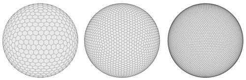
A DGGS expresses relationships between cells clearly through a consistent structure, producing a continuous surface at multiple resolutions. Cells of higher resolution are always related to cells of the lower resolution and vice versa. At aperture 3, a center point of a hexagon is also the center point of a cell at a higher resolution. A so-called hexagonal fishnet grid, as can often be found in geographical information systems, does not provide this capability especially at multiple scales. A transformation into raster space would encompass certain drawbacks. Raster data are popular for data cubes, but still do not fully articulate the fact that the earth is a sphere and not a plane. Also, pixels in a raster have four neighbors that share an ‘edge’ and four additional neighbors that only share a ‘node’. A DGGS therefore, is a way to make a consistent and structured cartographic argument. Compared to the boundaries of an administrative unit, a discrete global grid produces cell with similar cell geometry and identical cell topology, and thus a DGGS is more rational when fusing different types of data, such as points or attributes of areal units.

Point level data is simply aggregated to grid cells, but data from areal units such as administrative boundaries must be spatially interpolated. In this process, attribute data from areal units is split along the lines of the DGGS and the fractions of each unit are re-aggregated to the hexagonal cells, thereby transforming the source geometry into an abstract grid. Each cell of the grid is a location holding all the data as a table row with multiple attributes – telling the digital story of that place. The grid system fuses data from multiple sources into a data platform with a consistent spatial geometry. The consistent appearance of a location as a hexagon acknowledges the contingent and constructed nature of maps (Kitchin 2008; Kitchin and Dodge 2007; Kitchin, Gleeson, and Dodge 2013) while organizing the data in a format digestible by an ANN for predicting (sparse) phenomena.

2.2. Artificial neural network (ANN)

Machine learning efficiently processes structured input data such as images or tables with columns and rows. The DGGS format is a large table with one row per cell with a virtually endless number of associated attributes. We keep the spatiality, however, by converting the center points of each cell into columns for latitude and longitude; one can imagine these as two dimensions of the entire data set. The ANN learns iteratively by taking a sample of the data and applying weights and biases to the attributes of each cell until the algorithm crosses a threshold defined by the user, based on the learning rate and the number of epochs. Over multiple epochs, the algorithm gains modeling experience so that the prediction accuracy of the desired output attribute – the label – increases. We bring all attributes, the raw data, to the algorithm and let the ANN itself decides which, or what combination of attributes are significant, and which are not relevant (Goodfellow, Bengio, and Aaron 2016). The black-box nature of ANNs and calculations based on correlation, however, does not reveal causal relationships between attributes and predictive variables. These predictive results demand cross-validation, external verification, and thorough interpretation.

Artificial neural networks (ANN), also called deep learning (DL), are described and explained at length in (Hawkin 2014; Schmidhuber 2015; Nielsen 2015; Goodfellow, Bengio, and Aaron 2016) and reviewed in (Lecun, Bengio, and Hinton 2015). With the advancements in computer science and hardware development, neural networks have solved complex problems and reached unprecedented accuracy, e.g. predicting the location of a photo (Weyand, Kostrikov, and Philbin 2016). Especially image classification, pattern recognition, and object detection are popular areas of convolutional neural network research. The applications for deep learning range from finance, health, autonomous driving, to speech recognition and have permeated many of the data-driven fields. Geography, GeoScience and earth observation are no exception to this, as discussed in two book chapters in the ‘Manual of Digital Earth’: (Alderson et al. 2020) on ‘Digital Earth Platforms’ and (Guérin, Aydin, and Mahdavi-Amiri 2020) on ‘Artificial Intelligence’. While object detection from satellite images, or other remotely sensed imagery, receives much attention, comparatively little has been done on prediction of social phenomena. As many of the variables describing a society at a nation-wide level such as census information is not conveyed in imagery, nor are they in a data format that is easily digestible by a neural network, we opted for the previously described DGGS to prepare the data for the ANN. To evaluate the results of the ANN, a simple ordinary least squares regression is not sufficient, as it does not consider spatial relationships.

2.3. Spatial lag regression model (SLRM)

An ordinary least squares regression (OLS) between two variables does not consider the spatiality of the observations. Thus, spatial-autocorrelation effects that may influence the outcome of the regression are not considered. Spatial autoregressive models or spatial regression consider space in the calculation and are therefore suitable when dealing with geographic data. Borrowed from spatial econometrics, these concepts are amply explained in (Anselin and Rey 2014) and (LeSage 1999) and reviewed as an established method in (Anselin 2010). Common regression models that consider spatial dependence are geographically weighted regression (GWR), and spatial lag and spatial error regression models where the last two rely on a spatial weight matrix.

When estimating the correlation coefficient between two geographic variables, it is necessary to estimate the spatial dependence first. To do this, a so-called spatial weights matrix must be generated that conveys the information about neighboring entities by creating a list that specifies for each object under observation its neighbors. There are different methods to create a spatial weight matrix which are often contiguity or distance based. As an example, considering the state of Nevada, its direct neighbors would be Idaho, Utah, Arizona, California, and Oregon. This information about neighbors is stored in the spatial weights matrix and added as a term to the spatial regression model equation. The strength of the correlation is then expressed as a pseudo R²-value, comparable to the coefficient of determination in OLS regressions.

Using a DGGS proves to be a very suitable data framework when consistently generating the spatial weight matrix. As we use hexagonal cells, a contiguity-based weight calculation such as Queens or Rook, always produces six neighbors, at first order, that are also at an almost equal distance, producing comparable outputs across space. By increasing the order of the weights, more neighbors are included, not only those that touch the central cell under observation but also those further away. One computational problem that arises is the size of the spatial weight matrix for large spatial data sets. To overcome this problem, we use the spatial two stage least squares (S2SLS) generalized moments (GM) lag model that approximates maximum likelihood (ML) (Anselin and Rey 2014).

2.4. Processing chain

The main steps of the processing chain are data preparation, transform the input data into cells of a DGGS at all desired resolutions and join all sources into a master table. Feed the master tables multiple times into the ANN model fitting and evaluate the results with SLRMs. Any raw data, be it points, or polygons needs to be loaded into a spatial database system and transformed into the cells of the DGGS. This means polygons from e.g. administrative boundaries such as census tracts are stored as polygons, and points or postal addresses that need to be geo-coded are stored as points. All data sets are stored in their own table with their geometry (e.g. census tract) in a separate row. If the administrative boundary geometry is separated from the data table, a join based on a unique identifier is necessary, see Figure 2.

Figure 2. Flow chart of the entire process, the input data is transformed and re-aggregated to the cells of a DGGS, and then processed by the ANN. The SLRM evaluates the models.

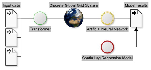
We transform the raw data tables into cells of the DGGS by intersecting points with the grid cells and by splitting polygons along the lines of the grid. We create a master table for each DGGS resolution, which aggregates the transformed input data into a table with many columns that hold the attributes. One column in the master table stores the attribute that should be predicted, this will be the so-called label for the artificial neural network model estimation. The ANN model uses the master table as an input. This table is split into a training and testing dataset, at a 50:50 ratio. Half of all the cells are used during model fitting, and the other half is used to test the model performance. Each attribute in the master table is scaled to the range 0–1 immediately before the model is run. We suggest running the model multiple times with batches that are 10% the size of the training dataset at cell sizes 50, 29, 17 and 10 km using this random sample of the data to train the model. After processing the master table in the ANN, a prediction result is achieved which needs to be rescaled to the original data range (the range of the label data). A spatial lag regression model will determine the result for each model run. We calculate the spatial weights matrix (Queens) with up to third degree neighbors for the SLRM.

3. Case study: predicting hate crimes

We explore the fuzzy and ill-defined social issue of hate crimes using machine learning to predict these incidents. While there is the hate crime statistics act (U.S.C. 1990), data availability at high spatial resolution for hate crime cases is sparse and uncertain. By employing a structured data platform, a DGGS, we can combine social and economic parameters as well as calculated parameters to predict hate crimes and validate the results of the model. The model learns based on a random sample of DGGS cells and outputs the predicted count of hate crimes for each cell. This allowed us to test the proposed model at different scales, as hate crimes and the underlying social and economic factors precipitating these incidents are scale dependent. We validated these results using a completely independent dataset.

We implemented a feed-forward neural network, also called multi-layer perceptron (MLP) to process the prepared data. This sequential model uses one densely connected input layer, one hidden layer and a single output cell to achieve a regression model that predicts a continuous value. We applied rectified linear unit (ReLU) activation for each layer. We compiled the model with a root-mean-square propagation RMSprop optimizer (Hinton, Srivastava, and Swersky 2014), with a learning rate of 0.00001, using the mean squared error metrics. The input data is shuffled and fed in batches during model fitting. As we run our model multiple times and want to keep the results as comparable as possible, we keep the learning rate low, and end the model estimation after 500 epochs.

To account for uncertainties in the ANN model estimation and to allow cross-validation of the results, we design the following strategy. We apply a 50:50 random split between training and testing data before the data is used in the neural network. In the specific case of this study, a 50% random sample of all the DGGS cells covering contiguous USA is used to train the model. We run the model 20 times at each of the four selected cell sizes with a diameter of ∼10 km to ∼50 km. With each iteration, another 50% random sample is used to train the model. This cross-validation approach ensures that the label (SPLC hate crime data) is always a sample. While the model optimization itself is not including spatial relationships (this would be against randomness) we tested the prediction result of the ANN against the original data collected by SPLC using a spatial lag regression model, see below. This determines a pseudo R²-value that considers spatial relationships in the regression.

3.1. Model data

We incorporated 454 demographic and economic variables expressed as percentages, including attributes such as income groups, veteran status, education by male and female, race and race change between 2000 and 2010, age groups by male and female and its change between 2000 and 2010, household composition, as shown in Table S1. A sample of these hate crime data predicted the probability of hate crimes in a specific location using an Artificial Neural Network (ANN). We scraped and geocoded data on hate & extremism about hate crimes for labelling and hate groups (Southern Poverty Law Center 2018) from the Southern Poverty Law Center (SPLC) data set[downloaded in 2017] (Southern Poverty Law Center 2017). Demographic data came from the US Department of commerce decennial census and five-year American Community Survey downloaded from National Historical Geographic Information System (NHGIS) (Manson et al. 2018) and data on police officer deaths in the line of duty from the officer down memorial page (ODMP) (The Officer Down Memorial Page (ODMP) 2018). We verified our analysis with the FBI hate crime statistics (Federal Bureau of Investigation 2017).

The Southern Poverty Law Center (SPLC) was an accessible source for hate crime data that did not aggregate cases at the state level. At the time of downloading, the website listed hate crimes including a date and postal address on their website. This database, is no longer available on the SPLC website. However, the SPLC recorded the data continuously in the past. The relative location, the postal address, of each hate crime is geo-coded to an absolute point location with latitude and longitude coordinates making it usable in a geographic information system (GIS) or spatial database. During geo-coding, several addresses could not be located definitively and were discarded. From the 4118 recorded hate crimes in the SPLC database, 3958 could be geo-coded and 2554 were used in the analysis after filtering. The data was collected between 16th January 2003 and 15th May 2015, to get the yearly average of 207 we divided by 12.33 (years).

Table S2 shows all hate crime types according to the SPLC database. From these types we only consider vandalism (1377 cases), assault (619), harassment (172), intimidation (111), threat (98), arson murder (74), cross burnings (45) and bombings (6) as those have corresponding categories in the FBI hate crime statistics which we use for verification, see section Validation data: FBI hate crime statistics. The SPLC hate crime types legal developments, leafleting, rally, intelligence and hateitude are excluded from our analysis because those are either not actual crimes (such as a rally) or the postal address may differ significantly from the actual location of the crime (such as legal developments).

In Table S3, we present other data sets on hate crimes that include spatial information from official and non-governmental (NGO) sources. To our knowledge, two NGOs collect and distribute data on hate crimes, The Anti-Defamation League (ADL) and the Southern Poverty Law Center (SPLC). Official datasets are published by the Federal Bureau of Investigation (FBI), the Uniform Crime Reporting (UCR), see section below, and the Bureau of Justice Statistics (BJS) in the National Crime Victim Survey (NCVS). We discuss all four datasets as they seem to be widely used in the literature (Adamczyk et al. 2014; Grattet and Jenness 2008) based on the five different criteria of accessibility, temporal scale, geographic scale, the number of incidents, and level of aggregation.

All data sets are accessible, but a noticeable difference is the number of cases collected by NGOs and official sources. While FBI UCR data are gathered from police departments in participating states and BJS NCVS through random sampling techniques in the US census, the SPLC and ADL can only rely on public information. The SPLC however, has the advantage of collecting data on hate crimes with high spatial resolution and enough temporal overlap between 2004 and 2015. A disadvantage of the BJS NCVS is the spatial unit of analysis and the lack of location information to geo-reference cases. BJS NCVS only mentions the site of an incident, such as ‘shopping mall’. FBI UCR has similar disadvantages as they aggregate data to sub-national units, not suitable for a more granular spatial analysis. The ADL collects data by city rather than census places.

We include hate group data collected by the Southern Poverty Law Center in this analysis (Southern Poverty Law Center 2018). The SPLC categorizes and observes the hate groups and adds them to their database. The SPLC records each hate group as a point with latitude and longitude coordinates (n=717), and only mentions the hate group type, not its number of members or date of establishment. This is inaccurate as a hate group may draw members from far away, and its range of actions may cover a larger territory than can be depicted with a point.

The Officer Down Memorial Page (ODMP) collects data about police officers that died in the line of duty since the 1800s (The Officer Down Memorial Page (ODMP) 2018). The ODMP provides each case with coordinates, which makes it suitable for our approach and may give insights, whether an area is prone to crimes and violence. We selected two subsets: one from 2000 to 2009 (n=1653) and one from 2010 to 2019 (n=1260) to have the most relevant cases in our model.

The Institute for Social Research and Data Innovation (ISRDI) at the University of Minnesota provides demographic and survey data through the National Historical Geographic Information System (NHGIS), in the Integrated Public Use Microdata Series (IPUMS) (Manson et al. 2018). We retrieved the decennial census data for 2000 and 2010, as this allows us to calculate variables about temporal change. The American Community Survey (ACS) data gives information about attributes like veteran status or household income. Table S1 presents all the subcategories with description. Each dataset has limitations as they are provided either at the point level or as areas of the shape of administrative units such as census tracts. The census data were converted to relative numbers to avoid telling the ANN about total population; additional predictive variables were calculated from the raw census numbers.

3.2. Data discretization

Data discretization was the strategy we adopted to mitigate some of the inherent problems of sparse data. Data discretization using a DGGS allowed us to integrate uncertain data from different sources into a consistent surface, subdivided into information units. The relationship of certain attributes such as hate crimes and hate groups may exhibit different patterns of spatial dependency at different scales (Openshaw 1983). For example, the area of influence of a event such as a hate crime is uncertain (Zhao, Kwan, and Zhou 2018) and the neighborhood effect is unclear (Kwan 2018). We discussed this in another paper titled ‘Mapping Crime – Hate crimes and hate groups in the USA: A spatial analysis with gridded data’ (Jendryke and McClure 2019), binning data was the strategy we adopted to deal not only with the problem of uncertain areas of influence but uncertainty in locational information concerning events.

This data discretization strategy was realized by an icosahedral aperture 3 DGGS with hexagonal cells at four different cell sizes. The resulting beehive-like pattern is an approximation to circular sampling, built as a hierarchical structure in which center points at lower resolution cells are also the centers of higher resolution cells. This consistency allows for the formation of a system of spatial units linked together across scales. For example, the hate crime locations were approximate; these stochastic events were initially treated as discrete points, but joined to DGGS cells for analysis given the locational uncertainty of the data. The multi-resolution approach, based on the DGGS system also enabled us to run the analysis at different scales. Granted, an analysis for the USA could have been done with a localized grid, properly projected to the USA, but our goal is to present a methodology for sparse data that would work globally without the need for adjustments.

Discrete global grids are standardized (Purss et al. 2016) and have certain advantages over other forms of data binning. The shape of the cells is irrelevant; triangles or quads would also be possible but we chose the hexagonal cells to be closer to a circular shape when modeling patterns of spatial autocorrelation. Moreover, DGGSs have a strong indexing schema which allows fast access to information, as well as fast access to cell parents, children, and neighbours thus reducing computational complexity and simplifying data pre-processing. In addition, machine learning can more efficiently process structured input data such as images or tables with columns and rows. The idea here is the leverage the potential of machine learning by preparing data in a format that is readable by basic ML algorithms. While computer vision takes raster images as an input, a feed forward network can process tabularized data as well. The cells of the DGGS are a way to create this structured table where each row is a cell, representing the spatial component in two columns for latitude and longitude along with other attributes in columns that describe the cell in terms of demography, social and economic factors or other phenomena, see section on ‘Artificial Neural Network (ANN)’ and ‘Model data’. The selected cell sizes have a refinement of sqrt (3), i.e. cells of a lower resolution are 1.72 times larger. This stepping is sufficient for our study, as we wanted to avoid too small or too big jumps from one resolution to the next but keeping the factor consistent.

3.3. Calculated parameters

As race may play a crucial role in predicting hate crimes, we calculated the Shannon diversity index (SDI) and the evenness index (EI) for 2000 and 2010 (Shannon and Weaver 1964). This is based on racial information in the demographic data. These indices reveal rather simplistically the diversity or evenness of a given area. The diversity index considers the number of races and the number of individuals for each census racial category. In theory, the artificial neural network should be able to identify the correlations between races if raw population counts are used in the model estimation. We calculate SDI and EI indices based on raw census numbers, with this equation, $SDI=-\sum (p_i\times \ln p_i)$where $p$ is the relative number of individuals of each race divided by the total number of samples. The EI is the SDI divided by the maximum SDI.

Another calculated parameter is the number of hate crimes in neighboring cells. This parameter is a way to estimate spatial dependence and neighboring effects between incidents. In crime research and crime prediction, knowledge of previous crimes is often used (Rummens, Hardyns, and Pauwels 2017) to make a prediction about future crimes. As we deal with very sparse data, a thorough temporal analysis that also includes geography is not possible. However, we can achieve a spatial co-occurrence indicator by summing the hate crime cases in neighboring cells for a cell under observation. As we deal with a hexagonal grid, the sum of all hate crimes in the six neighboring cells is used in this calculated parameter.

Looking at the raw hate crime counts as reported by the SPLC, we see that the cases over all cells follow a power-law probability distribution. Instead of taking the raw count of incidents, we multiply the hate crime count per cell by two and take the natural logarithm of the result. This modification of the so-called label minimizes the effect that few cells have a high number of recorded hate crimes while many cells have only a few reported incidents. Cells that have zero reported hate crimes still have zero hate crimes. This transformation is reversed once the model estimation and prediction of hate crime incidents is completed using $e$ and dividing by 2.

All datasets mentioned above are stored in a spatial database. Each attribute or group of attributes is joined with the cells of a DGGS by a unique identifier, as described in the next section. The result is a large table where each row is a DGGS cell and each column is an attribute. Spatial information is transferred to the model by using the latitude and longitude information of each cell’s center point. This structured format is suitable for an ANN. We applied a multi-scale approach and processed these tables for DGGS cells with different diameters. Altogether, 454 attributes were collected and calculated as listed in Table S1.

3.4. Validation data: FBI hate crime statistics

To verify our results against external data, we compared our predicted counts of hate crimes with the official FBI hate crime statistics using spatial regression at the state-level. In 1990, the US Congress passed the Hate Crime Statistics Act (28 U.S.C. § 534) to require the attorney general to collect information on hate crimes. The Hate Crime Statistics Act definition of hate crimes is ‘crimes that manifest evidence of prejudice based on race, religion, sexual orientation, or ethnicity.’ The Uniform Crime Reporting (UCR) is the mechanism to record hate crimes and while the data is public, a case-by-case dataset with hate crime type and a postal address that could be geo-coded is not accessible. Unfortunately, the public version of the FBI hate crime statistics lacks sufficient spatial information to carry out a thorough geographic investigation of the data. Instead, the data is aggregated at the state-level. For the presented study, we could download the data from 2011 to 2016, which temporally overlaps with the SPLC data, but the category names for hate crime are slightly different.

The categories in the original FBI hate crime statistics dataset are shown in direct matching to the SPLC hate crime types in Table S2. Considered are those that match the SPLC categories: murder and non-negligent manslaughter, aggravated assault, simple assault, intimidation, arson, destruction/damage/vandalism, and crimes against society.

4. Results and analysis

After preparing the aggregated datasets in the DGGS, we executed the Artificial Neural Network (ANN) 20 times at all four different cell sizes between ∼10 km and ∼50 km to capture and identify scale effects and to cross-validate and account for model uncertainties. All cells covering contiguous USA are randomly split 50:50 in each iteration for model training and testing, the results for model accuracy and precision are visualized in a two-panel box-plot diagram. We present our findings by selecting the results closest to the mean pseudo R²-value as determined by the spatial lag regression model and map the results for the predicted number of crimes per year, a risk map showing exposure to such incidents normalized by population, and a state-level map verifying our results with the official FBI hate crime statistics.

We visualize the accuracy and precision results of the model iterations in box-plot diagrams, presented in Figure 3 with additional information in Table S5 and Table S6. Panel A shows the pseudo R²-values as determined by a spatial lag regression model (SLRM), for the selected cell sizes. The mean pseudo R²-value of 0.4631 for cells with a diameter of ∼10 km rises to 0.7888 for cells with a diameter of ∼50 km. The narrow whiskers of the box plots indicate that the model accuracy is within a standard deviation of 0.0084 relatively stable over multiple iterations. Thus, the predictive accuracy of our model becomes greater with increasing DGGS cell sizes. We expect this, as the ratio between labeled cells that are not zero – cells that have no records of hate crimes – increases with larger cell diameter. A high pseudo R²-value means that our location prediction is accurate, but to evaluate the model precision, we must consider the total number of predicted hate crimes.

Figure 3. The artificial neural network ran 20 times at each cell size using a 50% sample of all cells covering contiguous USA. Panel A on the left shows the pseudo R²-values of the spatial regression between the recorded Southern Poverty Law Center (SPLC) hate crimes counts against the model prediction. The box plots are rather narrow, suggesting stable accuracy for all 20 iterations and cell sizes. With decreasing cell size, the accuracy of the model decreases. Panel B on the right shows the predicted number of hate crimes. The precision shows more variability; especially at cells size ∼29 km. With decreasing cell size, the model precision decreases as it tends to predict more hate crimes than actually recorded by SPLC.

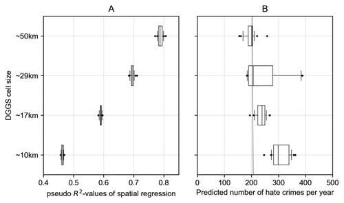
Panel B of Figure 3 shows the corresponding model precision by visualizing the spread of the total number of predicted hate crimes per year. The model predicted the number of hate crimes per year with more variation than expected. With smaller cell sizes, the model precision decreases. The median of the predictions for cells with a diameter of ∼50 km and ∼29 km was only off by −7 and 1 hate crime(s) from 207 cases per year reported by SPLC (red line). At the smallest cell diameters, the model predicts more than SPLC reported. This imprecision is due to the quality of the point level data put into the model. As cells get smaller, the associated attributes for neighboring cells become more similar; therefore, the model also predicts hate crimes in these neighboring areas regardless of the presence or absence of actual incidents in those cells.

From all 80 runs of the model we selected one to produce maps. While it would be feasible to create the average prediction of all 20 iterations at each DGGS cell size we select the one that is closest to the mean pseudo R²-value of that cell size. As we assume that the actual number of hate crimes is higher than what is reported by the SPLC and show a map with a cell size of ∼17 km here, maps of the other cell sizes are Figure S1, Figure S2, and Figure S3. The model is ∼59% correct and the spread of predicted incidents per year is within one standard deviation of just 18 incidents, thus balancing precision and accuracy with spatial resolution.

Figure 4 shows the predicted number of hate crimes per year for model run 13 at cells size 17 km. This run’s pseudo R2-value (0.5904) was the same as the mean of all pseudo R2-values for the cell size (Table S5). Darker shades of blue indicate a higher number of incidents, while lighter shades mean less or no incidents in grey. The highest number of predicted hate crimes was 5.88 incidents per year for a cell in New York.

Figure 4. This map shows the number of predicted hate crimes per year at DGGS cells size ∼17 km. We selected one artificial neural network run where the pseudo R²-value is closest to the mean of all iterations at this cell size as the result. Dark blue indicates more hate crimes, lighter shades less, and grey no hate crimes. The highest predicted number of hate crimes per year is 5.88 in New York City.

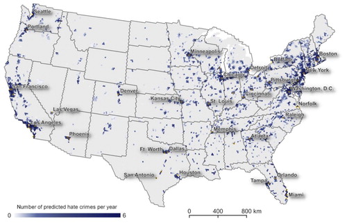
From the map in Figure 4, it becomes apparent that the predicted hate crime distribution is not random; clusters of higher density incident predictions are noticeable in the large urban agglomerations from Boston to Washington DC, Detroit to Chicago, and the larger Metropolitan areas on the west coast. The prediction however, does not show hate crimes in high density urban areas alone, but also in the southern states extending from Kansas City to Houston in the West to Atlanta and Norfolk in the East. This visual pattern may suggest that hate crimes strongly correlate with population density, but a spatial lag regression model between total population and the hate crime records from SPLC and alone results in a pseudo R²-value of 0.5542 while a regression between total population and the model prediction results in a pseudo R²-value of 0.6366, see Table S7. This prompts a comparison of the predicted number of hate crimes with the underlying total population to estimate the risk of experiencing a hate crime.

The map in Figure 5 shows the exposure to hate crime incidents by normalizing the prediction results shown in Figure 4 by the total population at cell size ∼17 km, maps of other cell sizes are in Figure S4, Figure S5, and Figure S6. Darker tones of red mean a higher frequency of up to 19 hate crime incidents per 10,000 people per year, while brighter tones mean fewer incidents per 10,000 people per year, and gray zero predicted hate crimes.

Figure 5. Normalizing the predicted number of hate crimes by total population results in a risk/exposure map. The map shows the risk of experiencing a hate crime; here for cells with ∼17 km diameter. Dark red indicates a higher risk of experiencing a hate crime, lighter shades less, and grey indicates little to no risk.

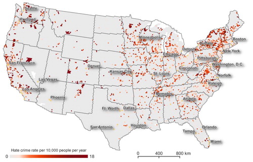
When normalizing the yearly predicted number of hate crimes with the underlying total population variations become visible, urban centers do not have highest exposure to hate crime. Looking at Boston, New York, Minneapolis, Atlanta, or Los Angeles we see a radial pattern of increasing exposure to hate crimes away from the center. The risk of experiencing a hate crime, according to our model, is higher towards the fringes of urban areas and between major agglomerations, for a detailed map see Figure S7. However, we must verify our prediction results against an independent dataset that has not been used in the model estimation.

A suitable source for independent verification is the FBI hate crime statistics; a dataset aggregated at the state-level that contains hate crime categories that can be matched to the SPLC data. While the FBI dataset contains 6316 hate crimes per year, the SPLC recorded only 207 hate crimes per year. To verify our findings, we summarize the prediction results of the ANN for cells with a diameter of ∼17 km per state (independent variable) and regressed it with the FBI hate crime statistics (dependent variable) using a spatial lag regression model (SLRM), see Figure 6.

Figure 6. To verify our results, we aggregate our predicted number of hate crimes at the state level. The residual of the spatial regression between the official FBI hate crime statistics and the model prediction shows that only 13 states have a standard deviation of more than ±1. Our results, while being overall lower in total number of predicted hate crimes, are 79% congruent with the FBI hate crime statistics.

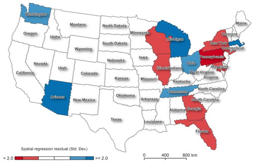
Out of 48 states and the District of Columbia that we used as units of analysis for verification 26% (13) had residual values that were greater or lesser than one standard deviation from the mean, suggesting a relatively high match between the model and the official FBI hate crime statistics for the time period tested. The states that are within one standard deviation account for ∼60% of the total population of the USA. Overall at the state level, the spatial lag regression model (SLRM) between our model prediction and the FBI hate crime statistics shows a strong fit with a pseudo R²-value of 0.7988, see Table S7.

5. Discussion and conclusions

We presented a theoretical framework that integrates data in a Discrete Global Grid System (DGGS), combines this data structure with an Artificial Neural Network (ANN) to predict sparse and uncertain events, and validates the results using spatial lag regression models (SLRM). From theory, we moved to a practical implementation that hierarchically bins demographic, economic, social attributes to grid cells of the DGGS. After feeding the DGGS with data we are able to train the ANN to make spatial predictions about a social event. This framework, however, is also able to ingest data from other sensors, such as earth observation imagery, social media data, or the Internet of Things (IoT), making it a generic approach to predict and correlate all kinds of (sparse) geographic phenomena. In our previous research on the relationship between hate groups and hate crimes in (Jendryke and McClure 2019) we realized that the prediction of hate crimes is complex and that more factors are at play. Hence, we developed the presented methodology to overcome the problems of data integration and machine learning. The DGGS that was used in the previous research proved to be a very suitable platform for application.

The data on hate crime incidents is uncertain and sparse, incidents are under-reported and the very term ‘hate crime’ is loosely defined, however despite these limitations it is possible to predict spatial patterns of hate crimes. These results need to be treated and interpreted with care as the reporting and recording of hate crimes is a politically contentious issue, undermining empirical investigations of this phenomenon. Analyzing the data on hate crimes from the Southern Poverty Law Center (SPLC) predicted aggregate occurrences at multiple scales, achieving a predictive capacity of up to 79%, for cells with a diameter of ∼50 km and 59% for cells with a diameter of ∼17 km. Our predictive maps show areas at risk of experiencing hate crime and are a guide to action for the police, civil society organizations, communities, and others combating violence and hate. Hate crimes are not spatially random, nor do they follow the population distribution, instead certain areas have a higher risk of experiencing hate crimes. One of the limitations and why further inspection of the prediction results is hampered is the fact that verification data at this level granularity does not exist. The only official source about hate crimes comes from the FBI and is only provided in state aggregated numbers at the national scale.

The areas with the highest exposure are those where urban areas transition from higher density to less urbanized (rural) areas. But an ANN only identifies correlations, it does not spell out one or few variables that explain events like hate crimes, thus no single variable is important. Even if we cannot say whether the selected variables are causal or just correlation, we conclude that machine learning can predict hate crimes at some degree of accuracy and precision. At the same time, a hexagonal grid replaces administrative boundaries as a unit of analysis and aggregation of uncertain data rather than distinct cases or neighborhoods. The results for hate crimes look promising, and the method will be applied to other types of events in future research.

This research can be improved with the addition of more comprehensive datasets on hate crimes at high spatial and temporal resolution, as we have not fully considered time in the presented study. Our method is not limited to the USA, nor is it fixed on predicting hate crimes per se. This method may be useful to make predictions about other phenomena such as epidemics, trade, migration, or conflicts where the data is sparse and uncertain by using other datasets and other labels that are relevant to the phenomenon. The results of the ANN model also require careful interpretation and the prediction numbers should not be taken as a reference for hate crimes, but as a guide to policymaking and civic engagement.

Acknowledgements

We would like to thank our colleagues, acquaintances, families and reviewers for their comments, criticisms, and support. Identifying information will be added after the review process.

Disclosure statement

No potential conflict of interest was reported by the author(s).

Data availability statement

Part of the data are not publicly available due to SPLC not offering data on hate crimes anymore. The data that support the findings of this study are available from the authors upon reasonable request.

Appendix

The Appendix document with supplementary material will be available at https://doi.org/10.1080/17538947.2021.1886356.

References

- Adamczyk, Amy, Jeff Gruenewald, Steven M. Chermak, and Joshua D. Freilich. 2014. “The Relationship Between Hate Groups and Far-Right Ideological Violence.” Journal of Contemporary Criminal Justice 30 (3): 310–332. doi:10.1177/1043986214536659.
- Adams, Benjamin. 2017. “Wāhi, a Discrete Global Grid Gazetteer Built Using Linked Open Data.” International Journal of Digital Earth 10 (5): 490–503. doi:10.1080/17538947.2016.1229819.
- Alderson, T., M. Purss, X. Du, A. Mahdavi-Amiri, et al. 2020. “Digital Earth Platforms.” Manual of Digital … . library.oapen.org. https://library.oapen.org/bitstream/handle/20.500.12657/23172/1006981.pdf?sequence=1#page=38.
- Amiri, Ali, Faramarz Samavati, and Perry Peterson. 2015. “Categorization and Conversions for Indexing Methods of Discrete Global Grid Systems.” ISPRS International Journal of Geo-Information 4 (1): 320–336. doi:10.3390/ijgi4010320.
- Anselin, Luc. 2010. “Thirty Years of Spatial Econometrics.” Papers in Regional Science 89 (1): 3–25. doi:10.1111/j.1435-5957.2010.00279.x.
- Anselin, Luc, and Sergio J. Rey. 2014. Modern Spatial Econometrics in Practice: A Guide to GeoDa, GeodaSpace and PySAL. Chicago.
- Byers, Bryan D., and Richard a. Zeller. 2001. “Official Hate Crime Statistics: An Examination of the ‘Epidemic Hypothesis.’.” Journal of Crime and Justice 24 (2): 73–85. doi:10.1080/0735648X.2001.9721135.
- Chen, Di, Miao Lu, Qingbo Zhou, Jingfeng Xiao, Yating Ru, Yanbing Wei, and Wenbin Wu. 2019. “Comparison of Two Synergy Approaches for Hybrid Cropland Mapping.” Remote Sensing 11 (3): 1–18. doi:10.3390/rs11030213.
- Djavaherpour, Hessam, Ali Mahdavi-Amiri, and Faramarz F. Samavati. 2017. “Physical Visualization of Geospatial Datasets.” IEEE Computer Graphics and Applications 38 (3): 61–69. doi:10.1109/MCG.2017.38.
- Espiritu, Antonina. 2004. “Racial Diversity and Hate Crime Incidents” 41: 197–208. https://doi.org/10.1016/j.soscij.2004.01.006.
- Federal Bureau of Investigation. 2017. “Uniform Crime Reporing - Hate Crime Statistics.” 2017. https://www.fbi.gov/services/cjis/ucr/hate-crime.
- Fuller, R. Buckminster, and E. J. Applewhite. 1976. “Synergetics: Explorations in the Geometry of Thinking.” Technology and Culture 17 (1): 104. doi:10.2307/3103256.
- Gale, L. R., W. C. Heath, and R. W. Ressler. 2002. “An Economic Analysis of Hate Crime.” Eastern Economic Journal 28 (2): 203–216.
- Gibb, R. G. 2016. “The RHEALPix Discrete Global Grid System.” IOP Conference Series: Earth and Environmental Science 34 (1): 1–8. doi:10.1088/1755-1315/34/1/012012.
- Gibson, Chris, Chris Brennan-Horley, and Andrew Warren. 2010. “Geographic Information Technologies for Cultural Research: Cultural Mapping and the Prospects of Colliding Epistemologies.” Cultural Trends 19 (4): 325–348. doi:10.1080/09548963.2010.515006.
- Goodchild, M. F., H. Guo, A. Annoni, L. Bian, K. de Bie, F. Campbell, M. Craglia, et al. 2012. “Next-Generation Digital Earth.” Proceedings of the National Academy of Sciences 109 (28): 11088–11094. doi:10.1073/pnas.1202383109.
- Goodfellow, Ian, Yoshua Bengio, and Courville Aaron. 2016. Deep Learning. Boston: MIT Press. http://www.deeplearningbook.org/.
- Gore, Al. 1998. “The Digital Earth: Understanding Our Planet in the 21st Century.” Australian Surveyor 43 (2): 89–91. doi:10.1080/00050326.1998.10441850.
- Grattet, Ryken, and Valerie Jenness. 2008. “Transforming Symbolic Law Into Organizational Action : Hate Crime Policy and Law Enforcement Practice.” Social Forces 87 (1): 501–527.
- Green, Donald P, Jack Glaser, and Andrew Rich. 1996. “From Lynching to Gay-Bashing: The Elusive Connection Between Economic Conditions and Hate Crime.” Journal of Personality and Social Psychology 75 (1): 82–92.
- Green, Donald P, Laurence H Mcfalls, and Jennifer K Smith. 2001. “Hate Crime: An Emergent Research Agenda.” Annual Review of Sociology 27: 479–504. doi:1/0811-0479.
- Green, Donald P., Dara Z. Strolovitch, and Janelle S. Wong. 1998. “Defended Neighborhoods, Integration, and Racially Motivated Crime.” American Journal of Sociology 104 (2): 372–403. doi:10.1086/210042.
- Grekousis, George. 2019. “Artificial Neural Networks and Deep Learning in Urban Geography: A Systematic Review and Meta-Analysis.” Computers, Environment and Urban Systems 74 (September): 244–256. doi:10.1016/j.compenvurbsys.2018.10.008.
- Guérin, Eric, Orhun Aydin, and Ali Mahdavi-Amiri. 2020. “Artificial Intelligence.” In Manual of Digital Earth, edited by Huadong Guo, Michael F. Goodchild, and Alessandro Annoni, 357–386. Beijing: SpringerOpen. https://www.springer.com/gp/book/9789813299146.
- Hawkin. 2014. Neural Networks and Learning Machines. ArXiv Preprint. https://doi.org/978-0131471399.
- Hinton, Geoffrey, Nitish Srivastava, and Kevin Swersky. 2014. “Lecture Notes: Neural Networks for Machine Learning.” University of Toronto. https://doi.org/10.1017/9781139051699.031.
- Jacobs, J. B., and K. A. Potter. 1997. “Hate Crimes: A Critical Perspective.” Crime and Justice 22 (May): 1–50. doi:10.1086/449259.
- Jefferson, Philip N., and Frederc L. Pryor. 1999. “On the Geography of Hate.” Economic Letters 65 (5): 389–395. doi:10.3917/reco.566.1249.
- Jendryke, Michael, and Stephen C McClure. 2019. “Mapping Crime – Hate Crimes and Hate Groups in the USA : A Spatial Analysis with Gridded Data.” Applied Geography 111: 1–10. doi:10.1016/j.apgeog.2019.102072.
- Katz, C. 1992. “All the World Is Staged: Intellectuals and the Projects of Ethnography.” Environment & Planning D: Society & Space 10 (5): 495–510. doi:10.1068/d100495.
- Kitchin, Rob. 2008. “The Practices of Mapping.” Cartographica 43 (3): 211–215. doi:10.3138/carto.43.3.211.
- Kitchin, Rob, and Martin Dodge. 2007. “Rethinking Maps.” Progress in Human Geography 31 (3): 331–344. doi:10.1177/0309132507077082.
- Kitchin, Rob, Justin Gleeson, and Martin Dodge. 2013. “Unfolding Mapping Practices: A New Epistemology for Cartography.” Transactions of the Institute of British Geographers 38 (3): 480–496. doi:10.1111/j.1475-5661.2012.00540.x.
- Kwan, Mei-Po. 2018. “The Limits of the Neighborhood Effect: Contextual Uncertainties in Geographic, Environmental Health, and Social Science Research.” Annals of the American Association of Geographers 4452 (May): 1–9. doi:10.1080/24694452.2018.1453777.
- Lecun, Yann, Yoshua Bengio, and Geoffrey Hinton. 2015. “Deep Learning.” Nature 521 (7553): 436–444. doi:10.1038/nature14539.
- Legewie, Joscha, and Merlin Schaeffer. 2016. “Contested Boundaries: Explaining Where Ethnoracial Diversity Provokes Neighborhood Conflict.” American Journal of Sociology 122 (1): 125–161. doi:10.1086/686942.
- LeSage, James. 1999. “Spatial Econometrics Toolbox.” http://www.spatial-econometrics.com/.
- Lin, Bingxian, Liangchen Zhou, Depeng Xu, A. Xing Zhu, and Guonian Lu. 2017. “A Discrete Global Grid System for Earth System Modeling.” International Journal of Geographical Information Science 00 (00): 1–27. doi:10.1080/13658816.2017.1391389.
- Mahdavi-Amiri, Ali, Erika Harrison, and Faramarz Samavati. 2015. “Hexagonal Connectivity Maps for Digital Earth.” International Journal of Digital Earth 8 (9): 750–769. doi:10.1080/17538947.2014.927597.
- Manson, Steven, Jonathan Schroeder, David Van Riper, and Steven Ruggles. 2018. “IPUMS National Historical Geographic Information System: Version 13.0 [Database].” University of Minnesota 2018. doi:10.18128/D050.V13.0.
- Medina, Richard M., Emily Nicolosi, Simon Brewer, and Andrew M. Linke. 2018. “Geographies of Organized Hate in America: A Regional Analysis.” Annals of the American Association of Geographers 108 (4): 1006–1021. doi:10.1080/24694452.2017.1411247.
- Mulholland, Sean E. 2013. “White Supremacist Groups and Hate Crime.” Public Choice 157 (1–2): 91–113. doi:10.1007/s11127-012-0045-7.
- Nielsen, Michael. 2015. Neural Networks and Deep Learning. Determination Press. http://neuralnetworksanddeeplearning.com/index.html.
- The Officer Down Memorial Page (ODMP). 2018. “Fallen Officer.” 2018. https://www.odmp.org/.
- Openshaw, Stan. 1983. The Modifiable Areal Unit Problem. Norwich: Geo Books. https://docplayer.net/21548943-Modifiable-areal-unit-problem-s-openshaw-issn-0306-6142-isbn-0-86094-134-5-s-openshaw.html.
- Pain, Rachel. 2015. “Social Geography : On Action- Orientated Research” 5 (2003): 649–57.
- Potere, David, Annemarie Schneider, Shlomo Angel, and Daniel L. Civco. 2009. “Mapping Urban Areas on a Global Scale: Which of the Eight Maps Now Available Is More Accurate?” International Journal of Remote Sensing 30 (24). doi:10.1080/01431160903121134.
- Purss, Matthew B.J., Robert Gibb, Faramarz Samavati, Perry Peterson, and Jin Ben. 2016. “The OGC® Discrete Global Grid System Core Standard: A Framework for Rapid Geospatial Integration.” International Geoscience and Remote Sensing Symposium (IGARSS) 2016-Novem: 3610–13. https://doi.org/10.1109/IGARSS.2016.7729935.
- Rose, Gillian. 1997. “Situating Knowledges: Positionality, Reflexivities and Other Tactics.” Progress in Human Geography 21 (3): 305–320. doi:10.1191/030913297673302122.
- Rummens, Anneleen, Wim Hardyns, and Lieven Pauwels. 2017. “The Use of Predictive Analysis in Spatiotemporal Crime Forecasting : Building and Testing a Model in an Urban Context.” Applied Geography 86: 255–261. doi:10.1016/j.apgeog.2017.06.011.
- Ryan, Matt E., and Peter T. Leeson. 2011. “Hate Groups and Hate Crime.” International Review of Law and Economics 31 (4): 256–262. doi:10.1016/j.irle.2011.08.004.
- Sahr, Kevin. 2011. ““Hexagonal Discrete Global Grid Systems for Geospatial Computing.” Archiwum Fotogrametrii.” Kartografii i Teledetekcji 22: 363–376. http://webpages.sou.edu/~sahrk/sqspc/pubs/sahrMMT11us.pdf%5Cnhttp://ptfit.sgp.geodezja.org.pl/wydawnictwa/krakow2011/APCRS vol. 22 pp. 363-376.pdf.
- Sahr, Kevin M. 2014. “Central Place Indexing : Optimal Location Representation for Digital Earth • Geospatial Computing Has Achieved,” 1–35.
- Sahr, Kevin M. 2017. Discrete Global Grid (DGG) Software.” http://www.discreteglobalgrids.org/. 2017. http://www.discreteglobalgrids.org/.
- Sahr, Kevin. 2019. “Central Place Indexing: Hierarchical Linear Indexing Systems for Mixed-Aperture Hexagonal Discrete Global Grid Systems.” Cartographica 53 (4): 16–29. doi:10.3138/cart.54.1.2018-0022.
- Sahr, Kevin, Mark Dumas, and Neal Choudhuri. 2011. “The PlanetRisk Discrete Global Grid System,” 1–5.
- Sahr, Kevin, Denis White, and A. Jon Kimerling. 2003. “Geodesic Discrete Global Grid Systems.” Cartography and Geographic Information Science 30 (2): 121–134. doi:10.1559/152304003100011090.
- Samavati, F. F., and T. Alderson. 2020. “Special Issue ‘Global Grid Systems.’” mdpi.com. https://www.mdpi.com/2220-9964/9/6/376/htm.
- Schmidhuber, Jürgen. 2015. “Deep Learning in Neural Networks: An Overview.” Neural Networks. https://doi.org/10.1016/j.neunet.2014.09.003.
- Shannon, Claude E., and Warren Weaver. 1964. The Mathematical Theory of Communication. https://doi.org/10.1145/584091.584093.
- Southern Poverty Law Center. 2017. “Hate Crimes.” https://www.splcenter.org.
- Southern Poverty Law Center. 2018. “Hate Map.” https://www.splcenter.org/hate-map#.
- Supp, S. R., Frank A. La Sorte, Tina A. Cormier, Marisa C.W. Lim, Donald R. Powers, Susan M. Wethington, Scott Goetz, and Catherine H. Graham. 2015. “Citizen-Science Data Provides New Insight Into Annual and Seasonal Variation in Migration Patterns.” Ecosphere, doi:10.1890/ES14-00290.1.
- U.S.C. 1990. Hate Crime Statistics Act. http://www.adl.org/issue_government/hate_crime_statistics_act.asp.
- Weyand, Tobias, Ilya Kostrikov, and James Philbin. 2016. “PlaNet - Photo Geolocation with Convolutional Neural Networks.” https://doi.org/10.1007/978-3-319-46484-8.
- Zhao, Pengxiang, Mei Po Kwan, and Suhong Zhou. 2018. “The Uncertain Geographic Context Problem in the Analysis of the Relationships etween Obesity and the Built Environment in Guangzhou.” International Journal of Environmental Research and Public Health 15 (2): 1–20. doi:10.3390/ijerph15020308.