Evaluation of stereology for snow microstructure measurement and microwave emission modeling: a case study

ABSTRACT

Reliable microstructure measurement of snow is a requirement for microwave radiative transfer model validation. Snow specific surface area (SSA) can be measured using stereological methods, in which snow samples are cast in the field and photographed in the laboratory. Processing stereology photographs manually by counting intersections of test cycloids with air–ice boundaries reduces the problems in binary segmentation. This paper is a case study to evaluate the repeatability of the manually stereology interpretation by two independent research groups. We further assessed how uncertainty in snow SSA influences simulated brightness temperature (T_B) driven by the Microwave Emission Model of Layered Snowpacks (MEMLS), and how stereology compares to Near Infrared (NIR) camera and hand lens. Data was obtained from two alpine snow profiles from Steamboat Springs, Colorado. Results showed that stereological SSA values measured by two groups are highly consistent, and the ground radiometer measured T_B at 19 and 37 GHz was successfully predicted (RMSE<3.8 K); simulations using NIR SSA and hand-lens geometric grain size (D_g) measurements have larger errors. This conclusion was not sensitive to uncertainty in the free parameters of T_B modeling.

KEYWORDS:

• Microwave radiometry
• snow
• stereology
• snow microstructure
• MEMLS

1. Introduction

Snow microstructure plays a critical role in snow hydrology and snow remote sensing; thus, methods to quantify snow microstructure in the field are of great importance. Snow microstructure governs many important snow physical properties such as thermal conductivity (Sturm et al. 1997), and radiative transfer properties for visible, near-infrared, and microwave wavelengths (Wiscombe and Warren 1980; Mätzler 1987). Snow microstructure is central to microwave remote sensing methods to estimate snow water equivalent (SWE) (Chang, Foster, and Hall 1987; Kelly 2009). Rott et al. (2013) and Rutter et al. (2019) discuss the importance of an accurate snow microstructure estimate to constrain the SWE retrieval from Ku-band radar, a leading candidate for proposed snow missions by multiple space agencies (Xiong et al. 2016; Derksen et al. 2019). Thus, objective, repeatable methods to measure snow microstructure in the field are critical.

The most traditional way to describe the snow microstructure is to use the geometric grain size (D_g), defined as the maximum extent of the prevailing grains (Fierz et al. 2009). D_g can be measured in the field using a ruled card and a loupe-style hand lens (Elder et al. 2009), or postprocessed from photos of dispersed snow grains on a ruled card (Lemmetyinen et al. 2016; Langlois et al. 2010). D_g measurement can still be subjective; in most cases, the natural snow structure is bonded. This structure must be disaggregated in the D_g measurement protocol, which may confound observer interpretation of particle dimension. In contrast, the snow specific surface area (SSA) metric begins with the assumption of a continuous snow medium, including both grains and bonds. Snow casts allow preservation of snow microstructure by displacing air space inside a snow sample with a suitable casting agent (see Section 4.3 for more details). Casts may be analyzed using either micro-Computed Tomography (CT; Pinzer and Schneebeli 2009; Ebner, Schneebeli, and Steinfeld 2015; Hagenmuller et al. 2016), or stereology (Davis and Dozier 1989; Wiesmann, Mätzler, and Weise 1998; Reber, Mätzler, and Schanda 1987; Matzl and Schneebeli 2010; Riche, Schneebeli, and Tschanz 2012) methods in the laboratory. Both approaches in principle allow for measurement of snow SSA and other microstructure properties directly, such as the density, two-point spatial auto-correlation function (ACF) and correlation length (L_c). The snow SSA can also be measured in the field using NIR photography (Matzl and Schneebeli 2006), contact spectroscopy (Painter et al. 2007), Shortwave Infrared (SWIR) integrating sphere (Gallet et al. 2009; Montpetit et al. 2012; Zuanon 2013; Gergely, Wolfsperger, and Schneebeli 2014) and Snow Micro-Penetrometer (SMP) (Proksch, Lowe, and Schneebeli 2015a), but these approaches generally require validation using laboratory methods applied to ‘snow casts’. The basis of the micro-CT is identical to medical x-ray CT: the sample is illuminated by x-rays, the transmitted signal is measured, and the interior structure of the sample is numerically reconstructed, in the form of a three-dimensional map of ice–air classification. While the CT approach has been widely used in recent years (Avanzi et al. 2017; Wiese and Schneebeli 2017; Ishimoto et al. 2018; Eppanapelli et al. 2019), a CT machine is expensive, and CT analysis includes specification of a threshold used to perform the ice–air segmentation (Hagenmuller et al. 2016). In contrast to the CT approach, stereology is based on photographed surface sections of snow sample. The stereology approach requires only a cold laboratory, a microtome and a camera, and is thus significantly more accessible than CT. Furthermore, the allowable sample size is less restrictive using stereology.

There are two approaches to stereology: one in which each pixel in the snow sample photographs is classified into ice or air, and one in which images are interpreted manually. The process of classifying each pixel into ice or casting agent is called the segmentation. A successful segmentation requires samples with only few air-bubbles and little recrystallization of casting agent (Matzl and Schneebeli 2010); otherwise, using a fixed threshold to do the classification will introduce errors. Indeed, threshold-determining methods like sequential filtering and energy-based approaches in Hagenmuller et al. (2016) essentially require a bi-modal histogram of pixel values. In contrast, manual interpretation of stereology images can be done far more accurately. It is regularly held for stereology applications in general (i.e. mostly outside of snow) that manual interpretation is more reliable than automated segmentation (Shain et al. 1999; Haass-Koffler, Naeemuddin, and Bartlett 2012; Phoulady et al. 2019). Even for images of samples that show casting agent recrystallization, the snow SSA can be measured by manually counting the intersections of a test system of cycloid lines overlaid on the photograph with the ice–air interfaces (Riche, Schneebeli, and Tschanz 2012). However, the repeatability of this approach for measuring snow SSA across different observers needs to be examined, which is the focus of this paper.

In this paper, the stereological method to measure snow SSA based on manually counting protocol was tested over a deep alpine snow at Steamboat, Colorado, US in 2010. The stereological photos were interpreted by two independent research groups, and the difference in measured snow SSA and how the difference propagates in the passive microwave brightness temperature (T_B) simulation were evaluated. Direct snow microstructure measurement is the key to support the physically-based remote sensing model simulations (Xiong et al. 2012; Malinka 2014), clarify complex relationships between different snow microstructure parameters (Löwe and Picard 2015; Chang et al. 2016) and reinforce the understanding of newly-observed snow signal characteristics (Leinss et al. 2016).

In this study, the snow microstructure was also measured by hand lens and a NIR camera to be compared with the stereology. We are interested in the performance of different methods to describe the small and large snow particle dimensions, and how the errors comprehensively influence the T_B of a deep natural snowpack of vertical inhomogeneity. The snow T_B was observed by a ground-based radiometer at 19 and 37 GHz, vertical polarization, at an incidence angle of 50°. The Microwave Emission Model of Layered Snowpacks (MEMLS) based on Improved Born Approximation (IBA) (Mätzler 1998; Mätzler and Wiesmann 1999) is used as the modeling tool. The microstructure assumption of MEMLS-IBA is compatible with SSA. The microstructure parameters measured by stereology, NIR photography and hand lens were converted to the exponential correlation length (L_e) required by MEMLS using both the conventional coefficients from previous literature and the optimized coefficients. We will further discuss the influence of soil parameters to modeling results.

2. Snow microstructure based on continuous snow medium assumption

There are several parameters that can be used to describe a continuous snow medium, including the surface areas, curvatures, chord length distributions, correlation lengths and two-point spatial Auto Correlation Functions (ACF) (Mätzler 2002; Krol and Löwe 2016). Surface area of snow refers to the area of ice–air interface. Correlation lengths are highly relevant to ACF. The later evaluates the correlation of two random points in the medium as a function of the displacement between these two points. Taking the dry snow medium as an example, the two points will be considered of high correlation if they are both occupied by ice or air pore, and will be considered of low correlation if one is occupied by ice and the other is occupied by air. ACF is from the statistics of multiple pairs of points in the medium. An equation to calculate ACF for dry snow can be found in Mätzler (1997).

The snow specific surface area (SSA) is usually defined as the ratio of the total surface area of ice (including grains, bonds, etc.) (unit: m²) to the total volume (unit: m³) or total mass (unit: kg) of ice. SSA in the former case is denoted as S_i (unit: m⁻¹) in our paper. The surface to volume ratio, S/V (unit: m⁻¹), represents the ratio of the total surface area of ice to the total volume of snow. S/V is related to S_i as: (1) $S/V=S_i\times v$(1) where, v (unitless) is the ice volume fraction, calculated by snow density divided by ice density.

In Debye, Anderson, and Brumberger (1957), it theoretically deducted the relationship between S/V and the derivative of two-point spatial Auto Correlation Functions (ACF) at zero displacement, and Mätzler (2002) utilized this derivative to define a parameter called the correlation length (L_c) as follows: (2) $L_c=-{{\left({\displaystyle \frac{dA(x)}{x}}\right)}^{-1}|}_{x=0}={\displaystyle \frac{4v(1-v)}{S/V}}$(2) where, A(x) is ACF. L_c is in mm.

A fit to ACF by an exponential function gives the exponential correlation length (L_e) (Mätzler 2002) which follows: (3) $A(x)=e^{-{\displaystyle \frac{x}{L_e}}}$(3) If the snow ACF strictly follows an exponential-shape curve, L_e equals L_c. However, it has been found by Mätzler (2002) and Krol and Löwe (2016) that, for natural snow samples, L_e and L_c can have different values when the slope of ACF is steeper or more flat near the origin. The reason is L_e fitted by ACF over the full domain represents a longer-range autocorrelation, whereas L_c determined near the origin is from autocorrelation over very short length scales. In this case, a scaling factor is required to convert L_c to L_e as shown below: (4) $L_e=\beta L_c$(4) Substituting Equation (4) into Equations (1) and (2) gives a conversion from S/V and S_i to L_e as: (5) $L_e=\beta {\displaystyle \frac{4v(1-v)}{S/V}=\beta {\displaystyle \frac{4(1-v)}{S_i}}}$(5) Using the measurement of snow samples from Weissfluhjoch, Davos, Switzerland by stereology, Mätzler (2002) found a mean value of β as 0.75, with a standard deviation of 0.15. For different samples, β varies from about 1.0 for depth hoar to 0.66 in average for fresh snow. From the recent experiment in Krol and Löwe (2016), the average β is 0.79, and they explained the difference is from the more depth hoar samples included. Krol and Löwe (2016) also found a second-order ACF parameter called the curvature length can be used to narrow down the uncertainty in β estimate. Then, β can potentially be linked to a measurable objective parameter instead of the grain shape classification.

3. Microwave emission model for layered snowpack (MEMLS)

3.1. Model introduction

A seasonal snowpack is fundamentally a layered medium (Colbeck 1991). In many cases, the snow microwave emission cannot be understood without the layered characteristics of snowpacks (Hall, Chang, and Foster 1986; Boyarskii and Tikhonov 2000; Durand et al. 2011). This has motivated the development of multi-layer radiative transfer models. In this study, we utilize the Microwave Emission Model of Layered Snowpacks (MEMLS) (Wiesmann and Mätzler 1999), one of the first multi-layer snow RT models established from extensive theoretical (Mätzler 1997; Mätzler 1998; Mätzler and Wiesmann 1999) and experimental (Wiesmann, Mätzler, and Weise 1998; Mätzler 2002) studies. The Improved Born Approximation (IBA) was used to calculate the MEMLS scattering coefficient, for its stronger physical basis and outstanding unbiased performance at different frequencies compared to the empirical MEMLS scattering coefficient (Pan et al. 2016).

MEMLS treats snow as a continuous medium composed of ice and air. To simplify the requirement for inputs, it assumes the snow ACF follows an exponential function as in Equation (3). MEMLS requires L_e, whereas the stereology provides S/V, NIR camera provides S_i and hand lens provides D_g. A conversion of these microstructure parameters is needed, and will be described as follows.

3.2. MEMLS driven by SSA measurements

The snow SSA measurements have been widely used to drive the radiative transfer (RT) models for the passive microwave brightness temperature (T_B) simulation (Brucker et al. 2011; Rutter et al. 2014; Roy et al. 2013; Proksch et al. 2015b; Sandells et al. 2017). The accuracy of the snow radiative transfer (RT) models is expected to be higher when the snow microstructure assumptions between the model and the measurement are closer. Commonly, a scaling factor is needed when the two assumptions diverge, like the difference between L_e and L_c in Mätzler (2002) and the difference between optical grain size from SSA and the diameter of identical ice spheres in DMRT-ML (Dense Media Radiative Transfer – Multi Layer model) (Picard et al. 2013) in Roy et al. (2013). Hereafter, the β value of 0.75, derived from the direct snow microstructure measurement, is mentioned as β_M, and will be considered as a literature-based reference value to support the conversions in Equation (5).

When β was derived from the optimization of T_B simulations, it was found to have larger variation range (Montpetit et al. 2013; Brucker et al. 2011), with the possibility being to compensate for errors from other sources. Montpetit et al. (2013) used a β of 1.3 for snow in Canada. Brucker et al. (2011) used a β of 2.08 for snow in Antarctica. Likewise, we also calculated an optimized β (called β_O hereafter) for our case.

3.3. MEMLS driven by geometric snow grain size measurements

To support the use of legacy D_g measurements, the empirical relationship between D_g and S was studied (Mätzler 2002; Langlois et al. 2010). It has been checked in Durand, Kim, and Margulis (2008), Pan et al. (2016) and Montpetit et al. (2013) that MEMLS can be driven by D_g measurements with a T_B RMSE of approximately 10 K.

Durand, Kim, and Margulis (2008) developed an empirical relationship based on the measurements in Mätzler (2002) as: (6) $L_e=\{\begin{array}{cc}{a}_0+a_1\ln D_g& (v>v_0\mathrm{and}{D}_g>D_{g0})\\ L_{e0}& (\mathrm{otherwise})\end{array}$(6) Where a₀ = 0.18 mm, a₁ = 0.09 mm, which were best-fit parameters for a logarithmic relationship between D_g and L_e. v₀ = 0.2, D_g0 = 0.125 mm, L_e0 = 0.05 mm, which were used to determine a fixed threshold L_e for low density, small grain size snow.

However, for the snow in Sodankylä, Finland, Pan et al. (2016) refitted a new set of coefficients as a₀ = 0.23 mm and a₁ = 0.13 mm from the fast SSA measurements, which gives higher T_B simulation performance compared to the Durand, Kim, and Margulis (2008)'s coefficients. Interestingly, the ratios of a₀ and a₁ between Pan et al. (2016) and Durand, Kim, and Margulis (2008) are close, with an average value of 1.36. Neglecting the slight shape difference, we added an optimized multiplication scaling factor, α, to Equation (6) as: (7) $L_e=\alpha L_e^D(D_g)$(7) where, $L_e^D(D_g)$ is the L_e estimated using Durand, Kim, and Margulis (2008)'s coefficients. An α of 1.0 is denoted as α_D. The optimized α is denoted as α_O.

4. Data and methods

We collected concurrent ground-based radiometric and snowpit measurements in the yard of the Storm Peak Laboratory (SPL), located in the Rocky Mountains, Colorado, USA, at 40°27′18″, −106°44′ 38″, 3220 m height above sea level. SPL is within the Rabbit Ears study area of the NASA Cold Lands Processes Experiment (CLPX) in 2002–2003 (Elder et al. 2009). The site is located at the top of a small mountain, in a fairly exposed area with high winds and low temperatures typical throughout the winter. Deep snowpacks commonly accumulate. The nearby SNOTEL snow pillow site ‘Tower’ (06J29S) reports an average SWE of 95.5 cm on April 1 (from 1975 to 2010). Our study period spanned three days, 21–23 February, 2010. From the nearby Tower SNOTEL site, there was no change in SWE (i.e. no precipitation). Within these three days, the daily maximum air temperature at Tower site (20 m lower than SPL) was −5 ∼ −9.4°C, and the daily minimum air temperature was −19.4 ∼ −15.5°C.

4.1. Radiometer data

In order to measure the snow microwave radiance, we used a ground-based version of the NASA Airborne Earth Science Microwave Imaging Radiometer (AESMIR) operating at 19 and 37 GHz (Kim 2009). We mounted the radiometer approximately 3.5 meters vertically above the soil-snow interface, with an incidence angle of 50° up from nadir. The antennas have a narrow Full Width Half Maximum (FWHM) beamwidth of 8°, such that footprint has an area of approximately $\pi \times 0.12\times 0.30{\mathrm{m}}^2$ on the snow surface and $\pi \times 0.24\times 0.60{\mathrm{m}}^2$ on the soil surface.

Only the vertically-polarized T_B was measured. We performed a two-point calibration once per day. On each day, a snap-shot measurement between 30 ∼ 60 min (warm-up and calibration time excluded) was conducted. All voltage measurements were integrated over thirty-second periods using a fast-sampling voltage meter. The measured average T_B at 19 GHz, vertical polarization is 247.5, 252 and 248 K from 21 to 23 February, respectively, and that at 37 GHz is 227, 233 and 231 K, respectively. We are confident in our T_B observations as the T_B values differed by only few K without new snowfalls when the radiometer was calibrated independently for each observation.

4.2. Snowpit data

The snowpits were excavated on 22 and 23 February near to the ground-based radiometer. The pit on 22 February was approximately two meters from the center of the field of view (FOV), whereas the pit on 23 February was excavated directly in the center of the radiometer FOV after the T_B measurement was made.

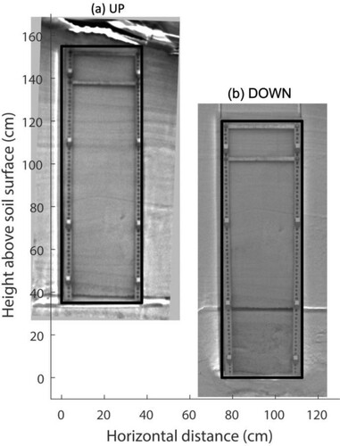
The wind-blown effect resulted in a slightly larger depth in the up-hill direction and a small depth in the down-hill direction. Therefore, we observed different pit depths of 174 and 165 cm on 22 and 23 February, respectively, with their SWE as 547 and 497 mm. The snowpits were evacuated perpendicular to the contour to capture the depth variability. As can be seen from the NIR photos in Figures 1 and 2, the landscape and the wind-blown effect resulted in some slant sub-interfaces which are not parallel to the ground. Therefore, the horizontal polarization was not explored to reduce the impacts on MEMLS simulation.

Figure 1. NIR photo of the snowpit on 22 February. The full snow profile was photographed two times. Firstly, a metal frame (37 × 120 cm size) was attached to the upper portion (a) of the profile and pictured; later, it was moved to the lower portion (b). Note that the topmost 12 cm was missed on this day when the snow was too loose to hold the frame.

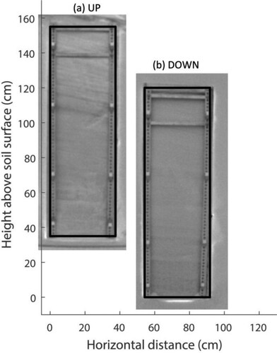
Figure 2. NIR photo of the snowpit on 23 February, photographed by the same method in Figure 1.

Stratigraphy of each pit was identified using standard snow hardness tests based on protocols established under the CLPX field campaign (Elder et al. 2009). There were six layers identified on 22 February and eight layers identified on 23 February (see Figure 3). Counted in the bottom-first order, layer 1 (the bottom layer) on both days was identified as depth hoar, and layer 2 was identified as composed of facetted crystals. These two bottom layers were followed by a few layers of faceted/round mix and rounds, and the topmost two layers were identified as new snow composed of partly decomposed precipitation particles. No ice lenses were found in both snowpits.

Figure 3. Stratigraphy, geometric grain size, and morphological classification according to Fierz et al. (2009) for the snowpits on 22 February (a) and 23 February (b).

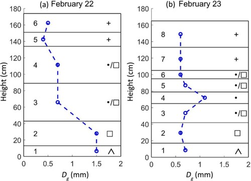
The geometric grain size (D_g) was measured using the aid of a loupe-style hand lens; following the CLPX grain size measurement protocol. The maximum and minimum dimensions of the large, medium and small snow grains were measured for each stratigraphic layer. The maximum dimension of the medium snow grains is closest to the definition of D_g in Mätzler (2002) and Fierz et al. (2009), written as the maximum dimension of the prevailing grains. Profiles of the measured D_g can also be found in Figure 3. It shows the measured D_g at the bottom of February 23 snowpit is much smaller than expected, albeit a depth hoar snow type. The reason will be discussed in Section 5.1. However, given the subjective nature of the D_g measurements, especially those from a hand lens, this discrepancy is unsurprising. Snow temperature was measured using a standard field thermometer to a precision of 1°C, at vertical increments of 10 cm. Snow density was measured to a precision of 1 kg m⁻³ by a wedge density cutter of 1000 cm³ volume.

4.3. Stereological analysis of snow samples

We made snow casts for stereological analysis. For each of the stratigraphic layers identified in the snowpit, a cubic sample of snow approximately 10 cm on each side was extracted. The vertical axis of each sample was noted on sample containers. We preserved the samples in the field using dimethyl phthalate dyed with Sudan black, following the procedure of Perla, Dozier, and Davis (1986). In the laboratory, samples were maintained at cold temperature below the melting point of the dimethyl phthalate during processing. Only the innermost section (∼20 × 8 × 8 mm) of each sample was analyzed, in order to minimize any effects of degradation near the edges. The sample was repeatedly cut (i.e. shaved back) parallel to the vertical direction in the snowpit using a microtome, and photographed by 1 mm step, twenty times. Cuts were made such that the sample face (8 × 8 mm) represents a vertical section defined in Riche et al.(2012). The ice and dimethyl phthalate dust was vacuumed with a shop vac attachment on the microtome to keep the sample clean. Photographs were made with a Canon EOS 60D 18 mpixel resolution camera with a Canon EF100 mm f/2.8 L macro lens illuminated by a ring light. Two photographs were taken of each face, one with a ruler of 1-mm grids overlaid in order to enable determining pixel size. Note that the samples were not thin sections, nor was the ice sublimated off.

Successful casts of layers 1–4 were made for 22 February, and successful casts of layers 1–5 were made for 23 February. Casts of the topmost layers (layers 5–6 February 22, layers 6–8 on February 23) were unsuccessful, as revealed by inspection of the snow section photographs. Therefore, L_e for these layers were estimated as follows. For Layer 5 and 6 on February 22 and layer 8 on February 23, L_e was estimated to be 0.05 mm, a typical value for fresh snow, referring to $L_{e0}$ in Equation (5). For layer 6 and 7 on February 23, L_e was assumed to be identical to layer 4 on February 22 because of similarity in D_g, density and height in the snowpit.

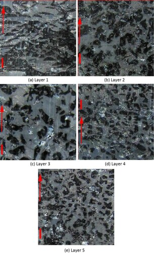
Figures 4 and 5 show one photograph (out of 20 in total) from each successfully-casted sample. Black pixels indicate ice, gray pixels indicate dimethyl phthalate originally occupied by pore space, and white pixels indicate either recrystallized dimethyl phthalate or air bubbles. Layer 1 on February 23 has some special horizontally-oriented thin structures, which were not observed in any other layers. This is from the side walls of connected, strongly striated, hollow depth hoar crystals. It has an observable difference with Layer 1 on February 22.

Figure 4. Stereological photographs of snow samples on February 22: (a) Layer 1 (depth hoar), (b) Layer 2 (facets), (c) Layer 3 (facets/round mix), (d) Layer 4 (facets/round mix). The vertical bar is a 1-mm ruler. The arrow indicates the upward direction in the snowpit.

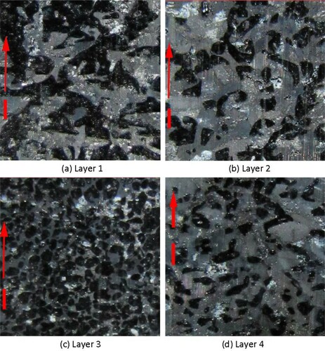
Figure 5. Stereological photographs of snow samples on February 23: (a) Layer 1 (depth hoar), (b) Layer 2 (facets), (c) Layer 3 (facets/round mix), (d) Layer 4 (rounds), (e) Layer 5 (facets/round mix).

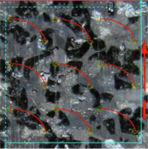
In order to calculate SSA, we used the methods explained and described in Matzl and Schneebeli (2010). The basic principle of the methodology is to overlay a test system of cycloids (following $x=2\theta -\sin 2\theta$, $y=1-\cos 2\theta$ for $0\le \theta \le \pi /2$) on each image: see Figure 6 as an example. An unbiased estimate of S/V can be retrieved using: (8) $S/V={\displaystyle \frac{2I}{d}}$(8) where, I is the number of intersections between the cycloids and the air–ice boundaries, and d is the cycloid length.

Figure 6. An example of cycloids overlaid on the stereological photo.

For validation purposes, the stereological counting was done by two separate research teams from Ohio State University (OSU) and Swiss Federal Institute for Forest, Snow and Landscape Research (WSL). The two groups overlaid the cycloids in different ways, but they both visually counted the intersections without doing binary segmentation. Ice volume fraction of the sample, v, in equation (5(5) $L_e=\beta {\displaystyle \frac{4v(1-v)}{S/V}=\beta {\displaystyle \frac{4(1-v)}{S_i}}}$(5) ) was calculated as the fraction of randomly-placed test points identified as ice in the stereological image.

The differences in the counting protocols from two research groups are as follows. First, the raw stereological photos were resized to coarser resolution to smooth the noise. Factors including the computer screen and the subjectivity of the observer influence pixel size. According to the 1-mm ruler, it turns out the pixel size from the OSU group was between 6.45 and 10.20 μm, whereas that from the WSL group was between 10.53 and 12.34 μm; both varied per photo. Second, the test system used by the OSU group includes 9 cycloids, and it used the two ends of cycloids (i.e. 18 test points) to calculate v. The WSL group used 25 cycloids to calculate S and 100 test points to calculate v. The cycloid length was ∼12.13 mm (177 pixels) used by the OSU group, and ∼7.66 mm (68 pixels) used by the WSL group.

4.4. Near infrared analysis of snow samples

In the field, a vertical wall of the excavated snowpit was photographed by a NIR camera to deliver the spatial information of SSA, following the procedure of Matzl and Schneebeli (2006).

The camera used to take NIR photo was a Canon G14. The wavelength of the detected light ranged from 840 to 940 nm, which is exactly the same as the camera used in Matzl and Schneebeli (2006). The distance between camera and pit wall varied between 1.4 and 2.0 m, resulting in an area of pit wall from 0.5 to 1.0 m². The ∼2 m depth snow pit wall was photographed by two parts (the upper and the lower part). See Figures 1 and 2. A metal frame was used to provide geometrical information and to mount pairs of Spectralon calibration targets of 50% and 99% reflectance. A semitransparent tarp was used to cover the pit hole to reduce direct sunlight. A flat white foam covering the pit wall was also photographed to correct the illumination difference of diffuse light.

The NIR reflectance, r, of the snow was calibrated using: (9) $r=a+bi$(9) where i is the illumination-corrected pixel intensity (digital numbers of pit wall photo divided by the white foam photo), and a and b are determined by a linear regression between i and the reflectance of calibration targets. Afterwards, S_i was calculated as (Matzl and Schneebeli 2006): (10) $S_i=A{e}^{r/t}$(10) where r is in %; A and t are empirical constants as 0.017 mm⁻¹ and 12.222, respectively.

The estimates of NIR S_i were averaged within each stratigraphic layer. The topmost part of the snow profile outside the metal frame (∼ 12 cm on February 22, ∼ 33 cm on February 23) was filled by the S_i right beneath that part, before processed to layer average. The v used to convert S_i to L_e was from snow cutter density measurements.

4.5. Optimization of conversion coefficients between snow microstructure parameters

As mentioned in the previous section, conversion coefficients are needed to convert S/V, S_i and D_g to L_e. Besides the literature-based conventional values, we calculated the optimized β_O and α_O using a cost function as: (11) $f_c=\sqrt{{\displaystyle \frac{(19v_M-19v_O{)}_{\mathrm{Feb}22}^2+(37v_M-37v_O{)}_{\mathrm{Feb}22}^2+(19v_M-19v_O{)}_{\mathrm{Feb}23}^2+(37v_M-37v_O{)}_{\mathrm{Feb}23}^2}{N}}}$(11) where, $19v_M$ and $19v_O$ are the predicted and observed T_B at 19 GHz, vertical polarization; $37v_M$ and $37v_O$ are defined similarly; N is the number of measurements, which is 4 in our case. $f_c$ is also the root-mean squared error (RMSE) of predicted T_B for two frequencies, two snowpits.

To run MEMLS, the downwelling sky brightness temperature was set as 21 and 33 K, respectively at 19 and 37 GHz, modeled by an 80% relative humidity under clear sky condition. The soil reflectivity was calculated by the Wegmüller and Mätzler (1999) model, using the bottom-most snow temperature as the physical temperature and a 0.1-cm soil roughness. The frozen soil dielectric constants were calculated using the Zhang et al. (2003) model. When Zhang et al. (2003) model was used, we used zero ice content and set the unfrozen volumetric soil water content (m_vu) was a free parameter. In the base simulation, a 12% m_vu was used, and later a sensitivity test was presented in Section 6.1.

5. Results

5.1. Comparison of snow microstructure measurements

Figure 7 shows the comparison of the measured S/V from stereological counting by the OSU and WSL groups. It shows the measured S/V from two research groups agreed with a mean relative difference of 2.7% and a root-mean squared error of 10%. The small difference from two research groups lends credence to the reliability of the stereological method. Tables 1 and 2 list S_i and L_c converted from S/V for the snowpits on February 22 and 23, respectively. To convert S/V to L_c, we used a single set of v from the WSL group. This is because WSL used 100 test points, whereas OSU used only 18 test points, and we found this difference caused approximately 11% systematically larger v from OSU than WSL. Such bias was not found for the S/V measurements. After conversion, the mean relative difference of L_c is −1.8%, and the root-mean squared difference is 8.8%.

Figure 7. Comparison of measured S/V calculated from Ohio State University (OSU) and Swiss Federal Institute for Forest, Snow and Landscape Research (WSL) groups.

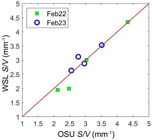
Table 1. Stereology analysis for the snowpit on February 22.

Layer# In Bottom-first Order	Ice Volume Fraction, v	Surface to Volume Ratio, S/V (mm^-1)		Specific Surface Area Per Ice Volume, Si (mm^-1)		Correlation Length, Lc (mm)
		WSL	OSU	WSL	OSU	WSL	OSU
1	0.429	1.95	2.12	4.54	4.94	0.503	0.462
2	0.312	1.99	2.48	6.38	7.93	0.431	0.347
3	0.410	4.35	4.33	10.61	10.56	0.223	0.223
4	0.243	3.01	3.03	12.37	12.47	0.245	0.243

Table 2. Stereology analysis for the snowpit on February 23.

Layer# In Bottom-first Order	Ice Volume Fraction, v	Surface to Volume Ratio, S/V (mm^-1)		Specific Surface Area Per Ice Volume, Si (mm^-1)		Correlation Length, Lc (mm)
		WSL	OSU	WSL	OSU	WSL	OSU
1	0.370	3.12	2.77	8.42	7.48	0.299	0.337
2	0.394	2.88	2.96	7.31	7.51	0.332	0.323
3	0.284	2.63	2.55	9.27	8.98	0.309	0.319
4	0.359	3.53	3.51	9.85	9.79	0.261	0.262
5	0.311	N/A	3.73	N/A	12.00	N/A	0.230

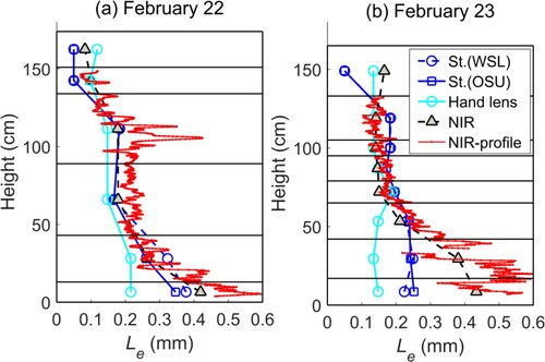
Figure 8 shows the comparison of the layered L_e converted from stereological S/V and NIR S_i measurements using β_M (as 0.75) and from D_g measurements using α_D (as 1.0). It also includes the fine-resolution NIR profile. There is a crack (at ∼ 37 cm height) observable on the February 23 pit wall from the NIR photo; thus the NIR data at this location was removed to reduce its influence on the L_e statistics. From Figure 8, first, it shows in general, the different estimates of L_e are well-correlated, with the exception of hand lens estimates for the bottom-most layer on February 22 and hand lens, stereological, and NIR estimates for the two bottom layers on February 23. Second, it shows the 0.05-mm L_e used for unsuccessfully-casted stereological samples at topmost layer is lower than the L_e estimates from NIR- and hand lens measurements. These assumed L_e for the stereological method may introduce errors to the T_B simulation, but we are also not confident on the other two methods, too. Third, for the bottom layer on February 23, some reasons for the differences can be found. As mentioned previously, the stereological counting was done independently by two different research groups. Therefore, we are confident in the stereological estimates. From the stereological photo in Figure 5(a), the special snow microstructure of Layer 1 on February 23 has a smaller dimension compared to that on February 22. It can result in the smaller D_g measured by hand lens and the larger S/V measured by stereology; in both cases, a smaller L_e is produced. However, comparison between the bottom part of NIR photos in Figures 1 and 2 show the crack and the rougher pit wall on February 23 can result in a decreased reflectance; in this case, a larger L_e is produced and diverges from the other two methods.

Figure 8. Profile of L_e using different measurement tools: (a) February 22, (b) February 23. St. represents stereology. For all methods, the conventional conversion coefficients are used.

5.2. Brightness temperature simulations

Figure 9 shows the error of the predicted T_B compared to the observed T_B, using L_e calculated from different measurements and conversion coefficients. Tables 3 and 4 list the T_B simulations. Table 5 summarizes the mean bias (MB), mean absolute error (MAE) and root-mean squared error (RMSE) of the predicted T_B.

Figure 9. Error of predicted T_B by MEMLS using L_e from different methods: (a) 19 GHz on February 22, (b) 37 GHz on February 22, (c) 19 GHz on February 23, (d) 37 GHz on February 23. In each subplot, from left to right, L_e is from: OSU stereology using β_M and β_O, WSL stereology using β_M and β_O, NIR photography using β_M and β_O, hand lens using α_D and α_O.

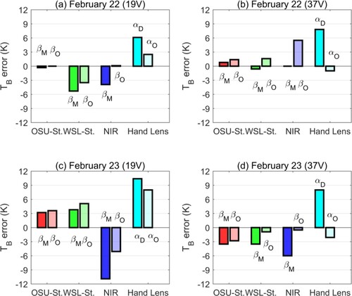
Table 3. Comparison of the measured and the MEMLS-predicted T_B using stereology, NIR camera and hand lens measurements, when L_e was converted by conventional conversion coefficients.

TB (K)	Scaling Factor	February 22		February 23
		19 GHz	37 GHz	19 GHz	37 GHz
Observed TB	–	252	233	248	231
Stereology-OSU	βM = 0.75	251.7	233.8	251.2	227.5
Stereology-WSL	βM = 0.75	246.7	232.4	251.8	227.5
NIR	βM = 0.75	248.1	233.0	237.1	225.0
Hand Lens	αD = 1.0	258.1	240.8	258.4	239.0

Table 4. Comparison of the measured and the MEMLS-predicted T_B, when L_e was converted by optimized conversion coefficients.

TB (K)	Scaling Factor	February 22		February 23
		19 GHz	37 GHz	19 GHz	37 GHz
Observed TB	–	252	233	248	231
Stereology-OSU	βO = 0.73	252.0	234.4	251.6	228.2
Stereology-WSL	βO = 0.72	248.5	234.6	253.1	230.1
NIR	βO = 0.68	252.1	238.5	242.9	230.5
Hand Lens	αO = 1.16	254.5	232.0	256.0	228.9

Table 5. Error Statistics of the MEMLS-predicted T_B using different snow microstructure measurements and L_e conversion coefficients.

Measurements	Scaling Factor	Mean Bias, MB (K)	Mean Absolute Error, MAE (K)	Root Mean Squared Error, RMSE (K)
Stereology-OSU	βM = 0.75	0.05	1.95	2.41
	βO = 0.73	0.55	1.95	2.39
Stereology-WSL	βM = 0.75	−1.40	3.30	3.71
	βO = 0.72	0.57	2.78	3.23
NIR	βM = 0.75	−5.20	5.20	6.52
	βO = 0.68	0.00	2.80	3.76
Hand Lens	αD = 1.0	8.08	8.08	8.22
	αO = 1.16	1.85	3.40	4.35

The observed T_B at 19 and 37 GHz is 252 and 233 K on February 22, and 248 and 231 K on February 23. Using OSU stereological measurements and β_M of 0.75, MEMLS predicts the observed T_B with a MB of 0.05 K and an RMSE of 2.41 K. An error value of 2.41 K is not far from the precision of the radiometer T_B measurements (∼2 K). The optimized β_O is 0.73, which is very close to 0.75. This optimization slightly reduced the RMSE from 2.41 to 2.39 K, but increased the MB from 0.05 to 0.55 K, which implies that the improvement from optimization is not significant. Therefore, it can be concluded that, the conventional β_M of 0.75 works for our snowpits, and the stereological measurements can be used to accurately estimate T_B. For the February 22 snowpit, MEMLS T_B accurately estimated both frequencies with an error of −0.3 and 0.8 K at 19 and 37 GHz, respectively. However, for the February 23 snowpit, T_B at 19 GHz is overestimated by 3.2 K and T_B at 37 GHz is underestimated by 3.5 K. According to the stronger penetration ability of the low frequency and the fact that T_B decreases with an increase of L_e, we would expect a slightly smaller L_e at the surface layers and a slightly larger L_e at the bottom layers to closely match the observed T_B.

From Figure 9, the T_B bias using WSL L_e is larger for both snowpits at 19 GHz; therefore, its RMSE (3.71 K) is slightly larger than OSU (2.41 K). However, a RMSE of 3.71 K is still quite acceptable. An optimized β_O for the WSL stereological measurements is 0.72. It reduced the MB from −1.40 to 0.57 K, the MAE from 3.30 to 2.78 K, and the RMSE from 3.71 to 3.23 K.

Using S_i measurements from NIR camera, the RMSE based on β_M is 6.52 K, and the ME is −5.2 K. As can be seen in Figure 8 and Table 3, a large difference between the simulation and the observation is from the February 23 snowpit, where the NIR pex is much larger than other methods and T_B at 19 and 37 GHz was underestimated by 10.9 and 6.0 K, respectively. The error for the February 22 snowpit is only −3.9 K and 0.0 K on two frequencies, respectively. It shows clearly that the much larger L_e derived from NIR photography for the bottom layers on February 23 contains some errors. An optimized β_O of 0.68 can reduce the RMSE from 6.52 to 3.76 K and MB from −5.2 to 0.0 K, but it degraded the accuracy at 37 GHz on February 22. This optimized β was influenced by a few poor microstructure measurements; thus, its value as a reference is reduced.

When L_e was converted from D_g measured by hand lens, the Durand's conversion coefficients result in an overestimation of 8.08 K in average. T_B at both frequencies and for both snowpits was overestimated. After optimization using an α_O of 1.16, it reduced the MB from 8.08 to 1.85 K, MAE from 8.08 to 3.40 K, and RMSE from 8.22 to 4.35 K. The α_O of 1.16 is between the Durand, Kim, and Margulis (2008) (α = 1.0) and the Pan et al. (2016) (α = 1.36) coefficients, and clearly represents a correction to systematic bias. After α was optimized, the biggest error comes from 19 GHz on February 23, which is 8 K overestimation. It indicates, albeit the systematic bias, the measured D_g at the bottom layers is still relatively underestimated. It agrees with the comparison with other measurement tools in Figure 8(b).

Overall, all the snow microstructure measurements, including S/V from the stereology, S_i from NIR photography and D_g from hand lens, give an RMSE below 9 K for T_B simulation without optimizing the L_e conversion coefficients. After optimization, it is possible to achieve an RMSE below 5 K using all measurements.

6. Discussions

6.1. Influence of soil parameters

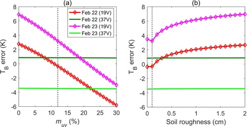
In this section, we evaluated the influences of the unmeasured soil moisture and soil roughness to errors of the predicted T_B. The range of soil parameters used for simulation is 0–30% unfrozen volumetric soil water content (m_vu) and 0–2 cm surface root-mean-squared (rms) height. Figure 10 shows the sensitivity of T_B error at two frequencies for both snowpits, when L_e is calculated using OSU stereological measurements and β_M. In general, it shows the influence of both soil parameters to T_B at 37 GHz is minor. This is expected because the snow is very deep. However, T_B at 19 GHz does remain some sensitivity to the soil parameters.

Figure 10. Error of the MEMLS predicted T_B as a function to unfrozen volumetric soil water content (m_vu) (a) and soil roughness (b). The vertical gray dash lines represent the 12% m_vu and 0.1 cm roughness used for simulations in Section 5.2.

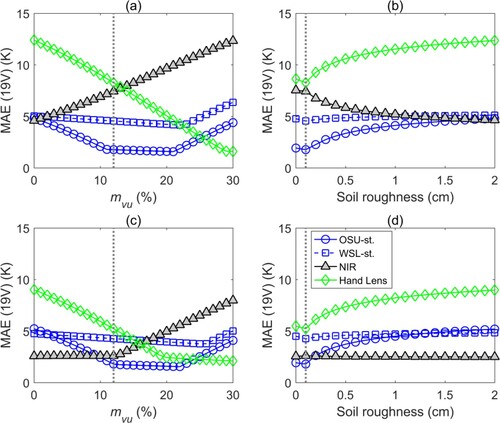
The second question needs to be addressed is, did the soil parameter values impose a seemingly better performance using the OSU stereological measurements than other measurements? To answer this question, Figure 11 shows the MAE at 19 GHz using different L_e as a function of soil parameters. In Figure 11(a,b), the conventional conversion coefficients were used. Clearly, it shows MAE varies with the soil parameter values. However, in a m_vu range of 0–25% and soil roughness range of 0–2 cm, the MAEs using OSU stereological measurements are always the smallest. In Figure 11(c,d) where the optimized conversion coefficients were used, the MAE using OSU serological measurements is no longer always the smallest, but still less than or comparable to at least two other types. Therefore, we can conclude that the highest T_B simulation performance from the utilization of stereological S/V is unaffected by soil parameter inputs and snow microstructure conversion coefficients.

Figure 11. Sensitivity of MAE of the predicted T_B at 19 GHz to unfrozen volumetric soil water content (m_vu) and soil roughness based on different microstructure measurements: (a)-(b) used the conventional coefficients, (c)-(d) used the optimized coefficients. st. represents stereology.

6.2. Influence of recrystallization to stereology

In this study, we observed the influence of recrystallization of casting agent on the stereological photo. The recrystallization leaves white spots on the sample sections, which covers or blurs the snow microstructure expected to be observed. Affected by the photo quality, the automatic segmentation by computer becomes unreliable. This is the most important reason why we only extracted S/V and S_i instead of the full ACF.

7. Conclusions

In this paper, an in-situ snow experiment was conducted at Steamboat Springs in Colorado mountain, US. The repeatability of stereological measurements was confirmed by comparing the estimates from two research groups based on seven samples from two deep snowpits, which contain both depth hoar and small facets/rounds. Later, the efficacy of the stereological measurements to predict the passive microwave T_B was evaluated. Results showed that the stereological measurement can be utilized to drive the Microwave Emission Model of Layered Snowpacks (MEMLS), a widely-used multi-layer snow radiative transfer model. MEMLS requires the exponential correlation length (L_e), whereas the stereology provides the surface to volume ratio (S/V). While the relationship between S/V and correlation length (L_c) is theoretical, an empirical fitting parameter is needed to further convert L_c into L_e. In this paper, we found the conversion coefficient β_M of 0.75 from the previous literature is usable for deep alpine snow in Colorado. It gives a RMSE of 2.41 and 3.71 K using the stereological measurements from the OSU and WSL research groups, respectively. This result highlights the utility of stereology to validate some more rapid SSA measurement tools in the context of microwave radiative transfer modeling.

The T_B modeling performance based on the stereological measurements was also compared with that based on NIR camera and hand lens measurements. The NIR camera measures the snow specific surface area per ice volume (S_i), and the hand lens provides the geometric grain size (D_g); they can also be used to drive MEMLS. Results showed that, using the conversion coefficients from previous literature without optimization, the T_B RMSE is below 9 K in all cases. It can be reduced to below 5 K after optimization; however, only the optimization for hand lens measured D_g represents a correction for a systematic bias.

When snow is composed of ice grains and grain bonds of different sizes, the snow specific surface area (SSA) is a general parameter that represents the total surface area of all components within a unit volume. Recent studies have shown that besides SSA, a second-order microstructure parameter to represent the grain size distribution is important for determining the snow ACF (Krol and Löwe 2016) and the microwave volume scattering (Chang et al. 2016). Such parameter can be the curvature length from the snow sample measurement (Krol and Löwe 2016), or the stickiness in DMRT models (Picard et al. 2013) in the RT model configuration level. Therefore, we look forward to more high-quality stereological or micro-CT measurements to answer these open questions. On the other hand, although the D_g measurement has some degree of subjective nature, its repeatability and objectiveness can be improved by postprocessing the photo of a large number of crystals over a ruled card. Using this protocol, it is possible to provide a grain size distribution to enrich the snow microstructure description using fast SSA measurements in field.

Acknowledgements

This work was supported by the NASA Terrestrial Hydrology Program under Grant no. NNX09AM10G and the Strategic Priority Research Program of Chinese Academy of Sciences under Grant no. XDA20100300. The authors would like to gratefully thank Ian McCubbin and Dr. Gannet Hallar for hosting us at Storm Peak Laboratory, Ty Atkins for his invaluable assistance with the radiometer, and Dan Berisford and Jennifer Petrzelka for their help in the snowpits. We would like to thank Abiyu Getahun for his work on the stereological processing.

Disclosure statement

No potential conflict of interest was reported by the authors.

Additional information

Funding

This work was supported by NASA Terrestrial Hydrology Program [grant number NNX09AM10G]; Strategic Priority Research Program of Chinese Academy of Sciences [grant number XDA20100300].

References

- Avanzi, Francesco, Giacomo Petrucci, Margret Matzl, Martin Schneebeli, and Carlo De Michele. 2017. “Early Formation of Preferential Flow in a Homogeneous Snowpack Observed by Micro-CT.” Water Resource Research 53 (5): 3713–3729. doi:https://doi.org/10.1002/2016WR019502.
- Boyarskii, Dmitriy A., and Vasiliy V. Tikhonov. 2000. “The Influence of Stratigraphy on Microwave Radiation from Natural Snow Cover.” Journal of Electromagnetic Waves and Applications 14 (9): 1265–1285. doi:https://doi.org/10.1163/156939300X01201.
- Brucker, Ludovic, Ghislain Picard, Laurent Arnaud, Jean-Marc Barnola, Martin Schneebeli, Hélène Brunjail, Eric Lefebvre, and Michel Fily. 2011. “Modeling Time Series of Microwave Brightness Temperature at Dome C, Antarctica, Using Vertically Resolved Snow Temperature and Microstructure Measurements.” Journal of Glaciology 57 (201): 171–182. doi:https://doi.org/10.3189/002214311795306736.
- Chang, Wenmo, Kunghau Ding, Leung Tsang, and Xiaolan Xu. 2016. “Microwave Scattering and Medium Characterization for Terrestrial Snow With QCA–Mie and Bicontinuous Models: Comparison Studies.” IEEE Transactions on Geoscience and Remote Sensing 54 (6): 3637–3648. doi:https://doi.org/10.1109/TGRS.2016.2522438.
- Chang, Alfred T., James L. Foster, and Dorothy K. Hall. 1987. “Nimbus-7 SMMR Derived Monthly Global Snow Cover and Snow Depth.” Annals of Glaciology 9: 39–44. doi:https://doi.org/10.3189/S0260305500200736.
- Colbeck, Samuel C. 1991. “The Layered Character of Snow Covers.” Reviews of Geophysics 29 (1): 81–96. doi:https://doi.org/10.1029/90RG02351.
- Davis, Robert E., and Jeff Dozier. 1989. “Stereological Characterization of Dry Alpine Snow for Microwave Remote Sensing.” Advances in Space Research 9 (1): 245–251. doi:https://doi.org/10.1016/0273–1177(89)90492-4.
- Debye, P., H. R. Anderson Jr., and H. Brumberger. 1957. “Scattering by an Inhomogeneous Solid. II. The Correlation Function and Its Application.” Journal of Applied Physics 28 (6): 679–683. doi:https://doi.org/10.1063/1.1722830.
- Derksen, Chris, Juha Lemmetyinen, Joshua King, Stephane Belair, C. Garnaud, M. Lapointe, Yves Crevier, G. Burbidge, and Paul R. Siqueira. 2019. “A Dual-Frequency Ku-Band Radar Mission Concept for Seasonal Snow.” 2019 IEEE International Geoscience and Remote Sensing Symposium (IGARSS 2019): 5742–5744, Yokohama, Japan, July 28–August 2. doi:https://doi.org/10.1109/IGARSS.2019.8898030.
- Durand, Michael, Edward J Kim, and Steven A Margulis. 2008. “Quantifying Uncertainty in Modeling Snow Microwave Radiance for a Mountain Snowpack at the Point-Scale, Including Stratigraphic Effects.” IEEE Transactions on Geoscience and Remote Sensing 46 (6): 1753–1767. doi:https://doi.org/10.1109/TGRS.2008.916221.
- Durand, Michael, Edward J. Kim, Steven A. Margulis, and Noah P. Molotch. 2011. “A First-Order Characterization of Errors from Neglecting Stratigraphy in Forward and Inverse Passive Microwave Modeling of Snow.” IEEE Geoscience and Remote Sensing Letters 8 (4): 730–734. doi:https://doi.org/10.1109/LGRS.2011.2105243.
- Ebner, Pirmin Philipp, Martin Schneebeli, and Aldo Steinfeld. 2015. “Tomography-Based Monitoring of Isothermal Snow Metamorphism Under Advective Conditions.” The Cryosphere 9 (4): 1363–1371. doi:https://doi.org/10.5194/tc-9–1363-2015.
- Elder, Kelly, Don Cline, Glen E. Liston, and Richard Armstrong. 2009. “NASA Cold Land Processes Experiment (CLPX 2002/03): Field Measurements of Snowpack Properties and Soil Moisture.” Journal of Hydrometeorology 10 (1): 320–329. doi:https://doi.org/10.1175/2008JHM877.1.
- Eppanapelli, Lavan Kumar, Fredrik Forsberg Forsberg, Johan Casselgren, and Henrik Lycksam. 2019. “3D Analysis of Deformation and Porosity of Dry Natural Snow During Compaction.” Materials 12 (6): 850. doi:https://doi.org/10.3390/ma12060850.
- Fierz, Charles, Richard L. Armstrong, Yves Durand, Pierre Etchevers, Ethan Greene, David M. McClung, Kouichi Nishimura, Pramod K. Satyawali, and Sergey A. Sokratov. 2009. The International Classification for Seasonal Snow on the Ground. IHP–VII, Technical Documents in Hydrology, No 83; IACS Contribution No 1, 80, Paris: International Hydrological Programme (IHP) of the United Nations Educational, Scientific and Cultural Organization (UNESCO).
- Gallet, Jean-Charles, Florent Domine, Charles S. Zender, and Ghislain Picard. 2009. “Measurement of the Specific Surface Area of Snow Using Infrared Reflectance in an Integrating Sphere at 1310 and 1550 nm.” The Cryosphere 3: 167–182. doi:https://doi.org/10.5194/tc-3-167-2009.
- Gergely, Mathias, Fabian Wolfsperger, and Martin Schneebeli. 2014. “Simulation and Validation of the InfraSnow: An Instrument to Measure Snow Optically Equivalent Grain Size.” IEEE Transactions on Geoscience and Remote Sensing 52 (7): 4236–4247. doi:https://doi.org/10.1109/TGRS.2013.2280502.
- Haass-Koffler, Carolina L., Mohammad Naeemuddin, and Selena E. Bartlett. 2012. “An Analytical Tool That Quantifies Cellular Morphology Changes from Three-Dimensional Fluorescence Images.” Jove-Journal of Visualized Experiments 66: e4233. doi:https://doi.org/10.3791/4233.
- Hagenmuller, Pascal, Margret Matzl, Guillaume Chambon, and Martin Schneebeli. 2016. “Sensitivity of Snow Density and Specific Surface Area Measured by Microtomography to Different Image Processing Algorithms.” The Cryosphere 10: 1039–1054. doi:https://doi.org/10.5194/tc-10-1039-2016.
- Hall, Dorothy K., Alfred T. Chang, and James L. Foster. 1986. “Detection of the Depth-Hoar Layer in the Snow-Pack of the Arctic Coastal Plain of Alaska, USA, Using Satellite Data.” Journal of Glaciology 32 (110): 87–94.
- Ishimoto, Hiroshi, Satoru Adachi, Satoru Yamaguchi, Tomonori Tanikawa, Teruo Aoki, and Kazuhiko Masuda. 2018. “Snow Particles Extracted from X-ray Computed Microtomography Imagery and Their Single-Scattering Properties.” Journal of Quantitative Spectroscopy & Radiative Transfer 209: 113–128. doi:https://doi.org/10.1016/j.jqsrt.2018.01.021.
- Kelly, Richard. 2009. “The AMSR-E Snow Depth Algorithm: Description and Initial Results.” Journal of the Remote Sensing Society of Japan 29 (1): 307–317.
- Kim, Edward. 2009. “The Airborne Earth Science Microwave Imaging Radiometer (AESMIR)-NASA's new Passive Microwave Airborne Imager.” 2009 IEEE sensors, Christchurch, New Zealand, October 25–28; 1725–1728. doi:https://doi.org/10.1109/ICSENS.2009.5398492.
- Krol, Quirine, and Henning Löwe. 2016. “Relating Optical and Microwave Grain Metrics of Snow: The Relevance of Grain Shape.” The Cryosphere 10: 2847–2863. doi:https://doi.org/10.5194/tc-10-2847-2016.
- Langlois, Alexandre, Alain Royer, Benoit Montpetit, Ghislain Picard, Ludovic Brucker, Laurent Arnaud, Patrick Harveycollard, Michel Fily, and Kalifa Goïta. 2010. “On the Relationship Between Snow Grain Morphology and In-Situ Near Infrared Calibrated Reflectance Photographs.” Cold Regions Science and Technology 61 (1): 34–42. doi:https://doi.org/10.1016/j.coldregions.2010.01.004.
- Leinss, Silvan, Henning Lowe, Martin Proksch, Juha Lemmetyinen, Andreas Wiesmann, and Irena Hajnsek. 2016. “Anisotropy of Seasonal Snow Measured by Polarimetric Phase Differences in Radar Time Series.” The Cryosphere 10 (4): 1771–1797. doi:https://doi.org/10.5194/tc-10-1771-2016.
- Lemmetyinen, Juha, Anna Kontu, Jouni Pulliainen, Juho Vehviläinen, Kimmo Rautiainen, Andreas Wiesmann, Christian Mätzler, et al. 2016. ““Nordic Snow Radar Experiment.” Geoscientific Instrumentation, Methods and Data Systems 5 (2): 403–415. doi:https://doi.org/10.5194/gi-5-403-2016.
- Löwe, Henning, and G. Picard. 2015. “Microwave Scattering Coefficient of Snow in MEMLS and DMRT-ML Revisited: the Relevance of Sticky Hard Spheres and Tomography-based Estimates of Stickiness.” The Cryosphere 9 (6): 2101–2117. doi:https://doi.org/10.5194/tc-9-2101-2015.
- Malinka, Aleksey V. 2014. “Light Scattering in Porous Materials: Geometrical Optics and Stereological Approach.” Journal of Quantitative Spectroscopy and Radiative Transfer 141: 14–23. doi:https://doi.org/10.1016/j.jqsrt.2014.02.022.
- Matzl, Margret, and Martin Schneebeli. 2006. “Measuring Specific Surface Area of Snow by Near-Infrared Photography.” Journal of Glaciology 52 (179): 558–564. doi:https://doi.org/10.3189/172756506781828412.
- Matzl, Margret, and Martin Schneebeli. 2010. “Stereological Measurement of the Specific Surface Area of Seasonal Snow Types: Comparison to Other Methods, and Implications for mm-Scale Vertical Profiling.” Cold Regions Science and Technology 64 (1): 1–8. doi:https://doi.org/10.1016/j.coldregions.2010.06.006.
- Mätzler, Christian. 1987. “Applications of the Interaction of Microwaves with the Natural Snow Cover.” Remote Sensing Reviews 2 (2): 259–387. doi:https://doi.org/10.1080/02757258709532086.
- Mätzler, Christian. 1997. “Autocorrelation Functions of Granular Media with Free Arrangement of Spheres, Spherical Shells or Ellipsoids.” Journal of Applied Physics 81 (3): 1509–1517. doi:https://doi.org/10.1063/1.363916.
- Mätzler, Christian. 1998. “Improved Bom Approximation for Scattering of Radiation in a Granular Medium.” Journal of Applied Physics 83 (11): 6111–6117. doi:https://doi.org/10.1063/1.367496.
- Mätzler, Christian. 2002. “Relation Between Grain-Size and Correlation Length of Snow.” Journal of Glaciology 48 (162): 461–466. doi:https://doi.org/10.3189/172756502781831287.
- Mätzler, Christian, and Andreas Wiesmann. 1999. “Extension of the Microwave Emission Model of Layered Snowpacks to Coarse-Grained Snow.” Remote Sensing of Environment 70 (3): 317–325. doi:https://doi.org/10.1016/S0034-4257(99)00047-4.
- Montpetit, Benoit, Alain Royer, Alexandre Langlois, Patrick Cliche, Alexandre Roy, N. Champollion, Ghislain Picard, Florent Domine, and R. Obbard. 2012. “New Shortwave Infrared Albedo Measurements for Snow Specific Surface Area Retrieval.” Journal of Glaciology 58 (211): 941–952. doi:https://doi.org/10.3189/2012JoG11J248.
- Montpetit, Benoit, Alain Royer, Alexandra Roy, Alexandra Langlois, and Chris Derksen. 2013. “Snow Microwave Emission Modeling of Ice Lenses Within a Snowpack Using the Microwave Emission Model for Layered Snowpacks.” IEEE Transactions on Geoscience and Remote Sensing 51 (9): 4705–4717. doi:https://doi.org/10.1109/TGRS.2013.2250509.
- Painter, Thomas H, Noah P Molotch, Maureen Cassidy, Mark Flanner, and Konrad Steffen. 2007. “Contact Spectroscopy for Determination of Stratigraphy of Snow Optical Grain Size.” Journal of Glaciology 53 (180): 121–127. doi:https://doi.org/10.3189/172756507781833947.
- Pan, Jinmei, Michael Durand, Melody Sandells, Juha Lemmetyinen, Edward Kim, Jouni Pulliainen, Anna Kontu, and Chris Derksen. 2016. “Differences Between the HUT Snow Emission Model and MEMLS and Their Effects on Brightness Temperature Simulation.” IEEE Transactions on Geoscience and Remote Sensing 54 (4): 2001–2019. doi:https://doi.org/10.1109/tgrs.2015.2493505.
- Perla, Ron, Jeff Dozier, and Robert E. Davis. 1986. “Preparation of Serial Sections in Dry Snow Specimens.” Journal of Microscopy 142 (1): 111–114. doi:https://doi.org/10.1111/j.1365-2818.1986.tb02744.x.
- Phoulady, Hady Ahmady, Dmitry Goldgof, Lawrence O. Hall, Kevin R. Nash, and Peter R. Mouton. 2019. “Automatic Stereology of Mean Nuclear Size of Neurons Using An Active Contour Framework.” Journal of Chemical Neuroanatomy 96: 110–115. doi:https://doi.org/10.1016/j.jchemneu.2018.12.012.
- Picard, Ghislain, Ludovic Brucker, Alexandre Roy, Florent Dupont, Michel Fily, Alain Royer, and C. Harlow. 2013. “Simulation of the Microwave Emission of Multi-Layered Snowpacks Using the Dense Media Radiative Transfer Theory: the DMRT-ML Model.” Geoscientific Model Development 6 (4): 1061–1078. doi:https://doi.org/10.5194/gmd-6-1061-2013.
- Pinzer, Bernd R., and Martin Schneebeli. 2009. “Snow Metamorphism Under Alternating Temperature Gradients: Morphology and Recrystallization in Surface Snow.” Geophysical Research Letters 36 (2): 1–4. doi:https://doi.org/10.1029/2009GL039618.
- Proksch, Martin, Henning Lowe, and Martin Schneebeli. 2015a. “Density, Specific Surface Area, and Correlation Length of Snow Measured by High-Resolution Penetrometry.” Journal of Geophysical Research 120 (2): 346–362. doi:https://doi.org/10.1002/(ISSN)2169-9011.
- Proksch, Martin, Christian Mätzler, Andreas Wiesmann, Juha Lemmetyinen, M. Schwank, Henning Löwe, and Martin Schneebeli. 2015b. “MEMLS3&a: Microwave Emission Model of Layered Snowpacks Adapted to Include Backscattering.” Geoscientific Model Development 8 (8): 2611–2626. doi:https://doi.org/10.5194/gmd-8-2611-2015.
- Reber, B., Christian Mätzler, and E. Schanda. 1987. “Microwave Signatures of Snow Crusts Modelling and Measurements.” International Journal of Remote Sensing 8 (11): 1649–1665. doi:https://doi.org/10.1080/01431168708954805.
- Riche, Fabiene, Martin Schneebeli, and Stefan A Tschanz. 2012. “Design-Based Stereology to Quantify Structural Properties of Artificial and Natural Snow Using Thin Sections.” Cold Regions Science and Technology 79–80: 67–74. doi:https://doi.org/10.1016/j.coldregions.2012.03.008.
- Rott, Helmut, Donald W. Cline, Claude Duguay, Richard Essery, Pierre Etchevers, Irena Hajnsek, Michael Kern, et al. 2013. “CoReH2O, a Candidate ESA Earth Explorer Mission for Snow and Ice Observations.” Proc. Earth Observation and Cryosphere Science workshop, ESA SP-712 (May 2013), Frascati, Italy, November 13–16, 2012.
- Roy, Alexandre, Ghislain Picard, Alain Royer, Benoit Montpetit, Florent Dupont, Alexandre Langlois, Chris Derksen, and N. Champollion. 2013. “Brightness Temperature Simulations of the Canadian Seasonal Snowpack Driven by Measurements of the Snow Specific Surface Area.” IEEE Transactions on Geoscience and Remote Sensing 51 (9): 4692–4704. doi:https://doi.org/10.1109/TGRS.2012.2235842.
- Rutter, Nick, Melody J. Sandells, Chris Derksen, Joshua King, Peter Toose, Leanne Wake, Tom Watts, et al. 2019. “Effect of Snow Microstructure Variability on Ku-Band Radar Snow Water Equivalent Retrievals.” Cryosphere 13 (11): 3045–3059. doi:https://doi.org/10.5194/tc-13-3045-2019.
- Rutter, Nick, Mel Sandells, Chris Derksen, Peter Toose, Alain Royer, Benoit Montpetit, Alex Langlois, Juha Lemmetyinen, and Jouni Pulliainen. 2014. “Snow Stratigraphic Heterogeneity Within Ground-Based Passive Microwave Radiometer Footprints: Implications for Emission Modeling.” Journal of Geophysical Research 119 (3): 550–565. doi:https://doi.org/10.1002/2013JF003017.
- Sandells, Melody, Richard Essery, Nick Rutter, Leanne Wake, Leena Leppänen, and Juha Lemmetyinen. 2017. “Microstructure Representation of Snow in Coupled Snowpack and Microwave Emission Models.” Cryosphere 11 (1): 229–246. doi:https://doi.org/10.5194/tc-11-229-2017.
- Shain, W., S. Kayali, D. Szarowski, M. Davis-Cox, H. Ancin, A. K. Bhattacharjya, B. Roysam, and J. N. Turner. 1999. “Application and Quantitative Validation of Computer-Automated Three-Dimensional Counting of Cell Nuclei.” Microscopy and Microanalysis 5 (2): 106–119. doi:https://doi.org/10.1017/S1431927699000069.
- Sturm, Matthew, Jon Holmgren, Max König, and Kim Morris. 1997. “The Thermal Conductivity of Seasonal Snow.” Journal of Glaciology 43 (143): 26–41. doi:https://doi.org/10.3189/s0022143000002781.
- Wegmüller, Urs, and Christian Mätzler. 1999. “Rough Bare Soil Reflectivity Model.” IEEE Transactions on Geoscience and Remote Sensing 37 (3): 1391–1395. doi:https://doi.org/10.1109/36.763303.
- Wiese, Mareike, and Martin Schneebeli. 2017. “Snowbreeder 5: A Micro-CT Device For Measuring the Snow-Microstructure Evolution Under the Simultaneous Influence of A Temperature Gradient And Compaction.” Journal of Glaciology 63 (238): 355–360. doi:https://doi.org/10.1017/jog.2016.143.
- Wiesmann, Andreas, and Christian Mätzler. 1999. “Microwave Emission Model of Layered Snowpacks.” Remote Sensing of Environment 70 (3): 307–316. doi:https://doi.org/10.1016/S0034-4257(99)00046-2.
- Wiesmann, Andreas, Christian Mätzler, and Thomas Weise. 1998. “Radiometric and Structural Measurements of Snow Samples.” Radio Science 33 (2): 273–289. doi:https://doi.org/10.1029/97RS02746.
- Wiscombe, Warren J., and Stephen G. Warren. 1980. “A Model for the Spectral Albedo of Snow. I: Pure Snow.” Journal of the Atmospheric Sciences 37: 2312–2733. doi:https://doi.org/10.1175/1520-0469(1980)037<2712:AMFTSA>2.0.CO;2.
- Xiong, Chuan, Jiancheng Shi, Marco Brogioni, and Leung Tsang. 2012. “Microwave Snow Backscattering Modeling Based on Two-Dimensional Snow Section Image and Equivalent Grain Size.” 2012 IEEE International Geoscience and Remote Sensing Symposium (IGARSS), Munich, Germany, November 12; 150–153. doi:https://doi.org/10.1109/IGARSS.2012.6351615.
- Xiong, Chuan, Jiancheng Shi, Lingmei Jiang, and Yurong Cui. 2016. “Global Mapping of Snow Water Equivalent with The Water Cycle Observation Mission (WCOM).” 2016 IEEE International Geoscience and Remote Sensing Symposium (IGARSS), Beijing, China, July 10–15; 7396–7399. doi:https://doi.org/10.1109/IGARSS.2016.7730929.
- Zhang, Lixin, Jiancheng Shi, Zhongjun Zhang, and Kaiguang Zhao. 2003. “The Estimation of Dielectric Constant of Frozen Soil-Water Mixture at Microwave Bands.” Proceedings of 2003 IEEE International Geoscience and Remote Sensing Symposium (IGARSS) (IEEE Cat. No.03CH37477), Toulouse, France, July 21–25 (4): 2903–2905. doi:https://doi.org/10.1109/IGARSS.2003.1294626..
- Zuanon, Nicolas. 2013. “IceCube, a Portable and Reliable Instruments for Snow Specific Surface Area Measurement in the Field.” Proceedings of International Snow Science Workshop Grenoble, Chamonix Mont-Blanc, France, October 7–11; 1021–1023.